On the analysis of chromatographic biopharmaceutical data by
curve resolution techniques in the framework of the area of feasible solutions.
Mathias Sawalla, Matthias R¨udtb, J¨urgen Hubbuchb, Klaus Neymeyra,c
aUniversit¨at Rostock, Institut f¨ur Mathematik, Ulmenstraße 69, 18057 Rostock, Germany
bKarlsruhe Institute of Technology, Institute of Engineering in Life Sciences, Fritz-Haber-Weg 2, 76131 Karlsruhe, Germany
cLeibniz-Institut f¨ur Katalyse, Albert-Einstein-Straße 29a, 18059 Rostock, Germany
Abstract
Monitoring preparative protein chromatographic steps by in-line spectroscopic tools or fraction analytics results in medium or large sized data matrices. Multivariate Curve Resolution (MCR) serve to compute or to estimate the con- centration values of the pure components only from these data matrices. However, MCR methods often suffer from an inherent solution ambiguity which underlies the factorization problem. The typical unimodality of the chromato- graphic profiles of pure components can support the chemometric analysis. Here we present the pure components estimation process within the framework of the area of feasible solutions, which is a systematic approach to represent the range of all possible solutions. The unimodality constraint in combination with Pareto optimization is shown to be an effective method for the pure component calculation. Applications are presented for chromatograms on a model protein mixture containing ribonuclease A, cytochrome c and lysozyme and on a two-dimensional chromatographic separation of a monoclonal antibody from its aggregate species. The root mean squared errors of the first case study are 0.0373, 0.0529 and 0.0380 g/L compared to traditional off-line analytics. The second case study illustrates the potential of recovering hidden components with MCR from off-line reference analytics.
Key words: pure component calculation, multivariate curve resolution, bio-pharmaceuticals, chromatography, unimodality, FACPACK.
1. Introduction
Chromatography in biopharmaceutical industry is of great importance not only as an analytical technique but also as a preparation method for pure materials [1, 2, 3]. A typical application is protein chromatography [1, 3]. The basis for protein fractionation are different retention times of proteins due to their specific elution behavior, but the resulting chromatograms typically do not achieve baseline separation of different species. Instead, a second, orthogo- nal analytical measurement method is necessary to interpret the preparative protein chromatograms [1, 4, 5, 6]. The analytical dimension is typically achieved by off-line reference analytics. Alternatively, selective quantification by spectroscopic tools has been investigated as potential method for process monitoring [7]. The analysis of measure- ments is often done manually and is by no means trivial. Typically, the results depend on the analyst interpreting the data. In-line spectroscopic measurements are analyzed with calibrated statistical models such as partial-least squares regression [7]. Here, significant resources have to be invested into model calibration. The quality of the analysis has a distinct impact on the reliability and reproducibility of the results from preparative protein chromatography.
Automated calibration-free tools for chromatographic data analysis can improve the data interpretation and can sup- port the reproducibility of the results [8]. Such tools should be capable to identify the number of species, to compute pure component factorizations, to exploit the existence of unimodal profiles within the decomposition process and, last but not least, to handle strongly interfering peaks. Ideally, the method should be robust with respect to variations of the observed retention times.
The solution of such data analytical problems is incumbent on multivariate curve resolution (MCR) methods [9, 10], which are effective tools for the analysis of spectroscopic and chromatographic data. MCR methods solve the pure component calculation problem, namely to reconstruct the (pure component) factors from mixed spectral or
Email: mathias.sawall@uni-rostock.de (Mathias Sawall), mruedt@icloud.com (Matthias R¨udt), juergen.hubbuch@kit.edu (J ¨urgen Hubbuch),klaus.neymeyr@uni-rostock.de(Klaus Neymeyr)
chromatographic data. Originally, MCR methods were developed to decompose spectral mixture data as reaction- accompanying series of IR/Raman or UV/Vis spectra into the contributions from the pure components [11, 12]. The application of MCR methods to chromatographic data to biopharmaceutical applications is comparatively new [13, 14, 15, 16].
Typically the focus of MCR-methods is on determining one, single factorization for the given (chromatographic) data, but no systematic analysis of the solution ambiguity is applied [13, 15, 17, 16]. It is worth stressing that MCR- methods by using constraint-based Pareto optimization techniques evade the issue of non-unique solutions [18, 19].
Consequently, the pure component factorizations as computed by the routines [20, 21] and others strongly depend on the active constraints and their relative weighting. Such a steering effect of validated constraints is very helpful. For chromatographic data the typical unimodal profile shape of single components can support the MCR analysis [22, 23].
The situation is more complex in the case of multiple components with overlapping profiles. Many solutions can exist, but most of them do not represent chemically and physically meaningful profiles.
The intention of this paper is to discuss the pure component factorization problem for chromatographic biopharmaceu- tical data on the basis of the so-called area of feasible solutions (AFS), [24, 25, 26, 27, 28, 29]. This permits a general approach for the analysis of the solution ambiguity of the pure component calculation problem. The application of this relatively young tool to chromatographic data and biopharmaceutical problems seems to be new. Our focus lies on analyzing the non-uniqueness of the solutions, on giving guidelines for the practical application of the methods and on interpreting its results. The AFS is a low-dimensional representation of all possible profiles that the factorization problem can have for a given data set. Being aware on the existence of a solution ambiguity can only be a first step.
A second step should be a reduction to a single, hopefully true and chemically correct decomposition. We show that for the given chromatographic data the unimodality constraint can serve as an effective reducer in order to find the desired solution. This work takes up the chemometric MCR-based analyses of [14, 16] on the pure component extrac- tion of preparative protein chromatograms and demonstrates the application of AFS-based chemometric analyses. We hope that the latter more general approach can provide a deeper insight into the problem of profile ambiguities and strategies how to select the correct solution.
1.1. Organisation of the paper
The paper is organized as follows. First, Section 2 introduces two experimental data sets for the subsequent method development and the numerical testing. Section 3 is of central importance. It introduces the theoretical background of the solution ambiguity underlying MCR methods and how it complicates the pure component calculation problem.
The computation of properly constrained factors with respect to penalty and regularization functions is explained in Sec. 3.3. Then Sec. 3.4 presents the AFS approach and the FACPACK software for AFS related computations. Finally, Sec. 4 reports on the results for the experimental data sets and discusses the questions concerning the identification of the number of absorbing and reconstructable components.
2. Materials & Methods
The following two experimental data sets accompany the method developments and numerical experiments:
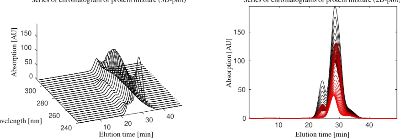
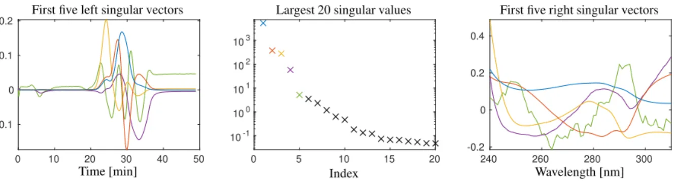
Data set 1. The first mixture contains the three model proteins, ribonuclease A, cytochrome c and lysozyme. The detailed data was previously published in [16]. Briefly, the UV/Vis-absorbance data of a cation-exchange chro- matography step from 240 nm to 310 nm was used for this study. A number of k = 588 spectra in the interval t∈[1.67·10−2,48.93] min were taken. Each spectrum consists of absorption values atn=71 wavelengths. The data (in 2D- and 3D-plots) as well as the singular value decomposition of the data matrix are shown in Figs. 1 and 3. (All numerical computations in this paper are done in MatLabversion R2018a and all singular value decompositions are computed by itssvd-routine.) MCR-based pure component factors under the constraint of unimodal elution profiles are shown in Fig. 5.
Data set 2. This data set describes a two-dimensional chromatographic separation of a monoclonal antibody (mAb) from its aggregate species. For technical details on this data set see [30]. The first chromatographic separation was based on preparative cation exchange chromatography (CEX) which is typically used in biopharmaceutical production processes for the purification of proteins [1]. However, preparative CEX only provides limited resolution of the different species. In order to specify the elution profiles, the effluent from the 5 column volume preparative CEX step was collected in fractions. These were then analyzed by a higher resolution second chromatographic separation (analytical size exclusion chromatography) to improve the resolution of the different species. During the second
0 50
300 100
280 150
260240 10 20 30 40
Elution time [min]
Absorption[AU]
Wavelength [nm]
Series of chromatogram of protein mixture (3D-plot)
10 20 30 40
0 50 100 150
Elution time [min]
Absorption[AU]
Series of chromatograms of protein mixture (2D-plot)
Figure 1: Series of chromatograms of a protein mixture according to data set 1 in a 3D-plot (left, only every third wavelength) and a 2D-plot (right, color changing from red to black with increasing wavelength values).
0 20 3 200 400
4 10 600
800
5 0
Retention time [min]
Absorption[AU]
Fraction
Series of chromatograms on monoclonal antibody separation (2D-plot)
3 3.5 4 4.5 5 5.5
0 200 400 600 800
Retention time [min]
Absorption[AU]
Series of chromatograms on monoclonal antibody separation (3D-plot)
Figure 2: Series of chromatograms of the separation of a monoclonal antibody (mAb) from its aggregate species according to data set 2. Left:
Series of chromatograms for the 20 fractions. Throughout this paper absorption values are given in AU for Arbitrary Unit. Right: Two-dimensional plot of the chromatographic profiles with a color changing from black to red with increasing fraction values.
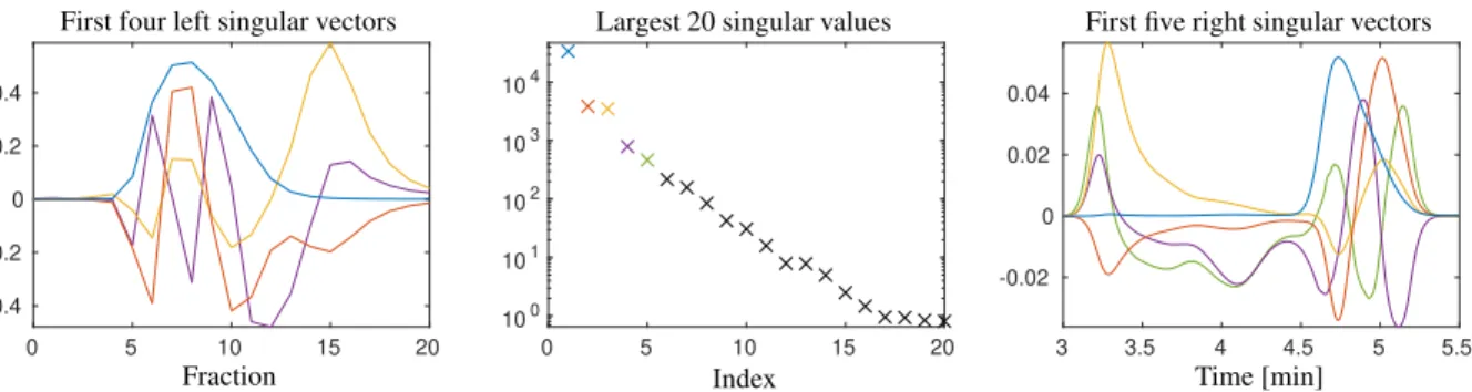
chromatographic separation, the UV absorbance trace at 280 nm was recorded. For the analysis we consider a number ofk=21 chromatograms each with absorption values atn=3751 retention times in the intervalt∈[3,5.5] min. The resulting series of analytical chromatograms are shown in two- and three-dimensional representation in Fig. 2. Figure 4 shows the dominant singular values and the associated singular vectors. The resulting pure component estimation is presented in Fig. 9.
3. Theory: The pure component calculation problem, its solution and solution ambiguties
The pure component calculation problem deals with the extraction of the pure component information (here chromato- graphic elution profiles) from the spectral or chromatographic mixture data. The series of spectra or chromatograms is stored row-wise in a matrixD ∈Rk×n. These data correspond to measurements on a retention time×wavelength grid or a retention time×fraction grid. The fraction axis can be considered as an intermediate coordinate for the sec- ond chromatographic separation. The naming of this coordinate is not important for the following analysis. Instead, we are interested in factorising the matrixDof mixture data to its source termsC ∈ Rk×s andS ∈ Rn×saccording the underlying bilinear structure of the problem. The dimensionsequals the number of components. This bilinear structure is expressed in the well-known Lambert-Beer law reading in matrix notation
D=CST+E. (1)
Ideally, the matrix E is the null matrix. In practice,E should be close to the null matrix and its non-zero entries express deviations from strict bilinearity, e.g., due to noise. The columns ofCare the concentration profiles in time of the pure components. Depending on the problem, the columns ofS are elution profiles, pure component spectra or other pure component profiles.
0 10 20 30 40 50 -0.1
0 0.1 0.2
Time [min]
First five left singular vectors
0 5 10 15 20
10-1 100 101 102 103
Index
Largest 20 singular values
240 260 280 300
-0.2 0 0.2 0.4
Wavelength [nm]
First five right singular vectors
Figure 3: The dominant singular values and associated singular vectors by an SVD of the matrix underlying data set 1. The largest/dominant singular value and the associated singular vectors are drawn blue. Then with a decreasing size of the singular values the colors red, ochre, purple and green are used. The singular values indicate that at leasts=3, but not more thans=4 components can be reconstructed.
3.1. Pure component calculation and the non-uniqueness of solutions
The problem of recovering the unknown pure component factorsCandS from the measuredDis a so-called inverse problem, which is closely related to the blind source separation problem [31] or the cocktail party problem [32]. Only matricesC andS with nonnegative entries can make physical sense. Thus D = CST poses a nonnegative matrix factorization problem for the given matrixD. See the monographs [9, 10] for a detailed introduction to MCR for applications in chemistry.
The nonnegative matrix factorization problem is not easy to solve. A main hurdle is the non-uniqueness of the solution of such factorization problems. In order to explain this non-uniqueness letD=CST be a nonnegative matrix factorization (NMF) ofDwhich means thatC,S ≥0. Typically many invertible matricesR∈Rs×sexist so that
D=CST =(CR−1)(RST)=CeeST (2)
is also a nonnegative factorization ofDwith the factorsCeandeS. Trivial examples of suchRare those that can be formed as a product of a permutation matrix and a diagonal matrix with positive diagonal elements. These matrices are called generalized permutation matrices and effect simultaneous permutations of the columns ofCandS together with mutual up- and down-scaling of the columns. These operations do not yield any additional information on the pure components, but correspond to an interchange of the components together with a scaling. More importantly, often other feasible matricesRexist that are different from generalized permutation matrices. From the viewpoint of the chemical MCR problem this solution ambiguity is very disturbing as only very few (if not only one) factorizations exist which have a chemical meaning. In the research field of chemometrics this problem of non-uniqueness is known under the keyword ofrotational ambiguity, see [11, 10, 19, 26, 29] among many others.
3.2. Reconstruction by singular value decomposition
Many methods for estimating the pure components are based on a singular value decomposition (SVD) ofD, see [33].
The SVDD=UΣVTis a three-factor decomposition ofDwhereU∈Rk×kandV∈Rn×nare orthogonal matrices and Σ∈Rk×nis a (rectangular) diagonal matrix. The diagonal elements ofΣare the singular valuesσ1 ≥σ2 ≥ · · · ≥0.
The columns ofUare called the left singular vectors ofDand the columns ofVare called the right singular vectors ofD.
IfDhas the ranks, then only its firstssingular values are positive and the remaining singular values equal zero. Then Dcan be represented only by the firstsleft and the firstsright singular vectors and the associated singular values; for smallsthis corresponds to an effective data compression. In the case of noisy experimental data the rank-smatrixD is perturbed by noiseDe=D+E. Typically,Dehas the maximal rank rank(eD)=min(k,n). If the noise level is small, then its firstslargest singular values dominate the remaining singular values which are close to zero. The SVD is the starting point for the construction of noise-filtered low rank approximations ofD. Only the firstssingular vectors carry important structure information and the remaining singular vectors with their associated close-to-zero singular values can be ignored. This amounts to a low-rank approximation ofDebyD. For data sets 1 and 2 the two figures 3 and 4 show the largest twenty singular values and the singular vectors belonging to the dominant singular values.
For experimental spectral data the size distribution of the singular values helps to determine the number of dominant, structurally important singular valuess. This number is the barrier to the remaining close-to-zero singular values that have their origin in noise. Usually,sis much smaller thankandn. Then the so-calledtruncated SVDis formed only
0 5 10 15 20 -0.4
-0.2 0 0.2 0.4
Fraction
First four left singular vectors
0 5 10 15 20
100 101 102 103 104
Index
Largest 20 singular values
3 3.5 4 4.5 5 5.5
-0.02 0 0.02 0.04
Time [min]
First five right singular vectors
Figure 4: The dominant singular values and associated singular vectors by an SVD of the matrix underlying data set 2. Three dominant singular values can be assumed, but there is no clear break-point between the dominant singular values and those close-to-zero singular values which are to be associated with noise.
by thesdominating singular values and the associated singular vectors. By using the same variable names also for the truncated matrices, namelyU∈Rk×s,V ∈Rn×sandΣ∈Rs×s, the factorization approach (2) finds its pendant in
D=UΣVT =UΣT| {z −1}
C
T VT
|{z}
ST
=CST. (3)
ThereinT is an invertible s-by-smatrix; for details see [11, 10, 34]. The main advantage of this approach is the reduction of the degrees of freedom. A direct computation ofCandS includes (n+k)svariables. In contrast to this, the representation of (3) reduces the degrees of freedom to thes2 matrix elements ofT. Equation (3) is the pivotal point for the optimization-based solution of MCR problems by using penalty and regularization functions in Sec. 3.3 and for the general analysis of the set of all nonnegative factorizations ofDin Sec. 3.4.
3.3. Optimization-based solution of the MCR problem
The computation of meaningful, chemically interpretable pure component factorizations is by no means trivial [18].
Sometimes additional information on the expected structure of the pure component factors is available which can help to steer the factorization process in a way that the pure component profiles are meaningful and interpretable.
Such a control of the factorization process can be achieved by a weighted sum of penalty and regularization terms [35, 12, 34, 16]. The idea is to minimize the reconstruction error D−CST under the constraints thatC andS are nonnegative matrices plus further constraints. Technically, this is implemented by considering the optimization problem
f(T)→min with f(T)=kD−CSTk2F+α1kmin(0,C)k2F+α2kmin(0,S)k2F+ Xp
i=1
βigi(C,S)2. (4)
Therein,k · k2F denotes the Frobenius norm, which is the sum of squares of all matrix elements of its matrix argument.
The coefficientsα1, α2 >0 are weight factors that determine how strongly the nonnegativity ofCandS is enforced.
Further regularization termsgi,i=1, . . . ,p, with weightsβi≥0 andβi≪α1, α2can be added.
Due to the representation ofCandS by (3) the residual termkD−CSTk2F can be replaced bykIs×s−T−1Tk2Fwithout changing the result of the optimization sincekD−CSTk2F =kIs×s−T−1Tk2F+Pmin(k,n)
i=s+1 σ2i and the latter term is a fixed value not influencing the minimum point. ThereinIs×sdenotes thes-by-sidentity matrix. In the case of noisy data a strict penalization of negative entries ofCorS can be too rigorous. Instead, small positive control parametersεC, εS
can be used that define lower boundaries on acceptable negative entries ofCandS in the form of relative size limits minC(:,i)
maxC(:,i)≥ −εC, minS(:,i)
maxS(:,i) ≥ −εS, i=1. . . ,s. (5)
The numerical minimization of the objective function f by (4) can be achieved by optimizers as the FORTRAN routineNL2SOLby ACM or the MatLabroutinelsqnonlin. Sometimes a pre-optimization by a genetic algorithm is worthwhile. If the data includes not only small deviations from the bilinear model (1), then it can be useful to use a higher number of singular vectorsz>sin order to reconstruct thespure component profiles [36, 34]. Such an approach is used if significant information on certain profiles cannot be extracted only from the firstssingular vectors.
Later we use this technique for data set 2.
The final success of such a Pareto optimization approach depends first and foremost on a proper selection of the regu- larization functions and their weighting. An imbalanced weighting can prevent convergence to meaningful solutions.
For strongly rectangular data sets withk≪norn ≪k, as this is the case for data set 2, the weight factors should be adapted properly. The unimodality constraint is of special importance for the analysis of chromatographic profiles in this work. The choice of the weighting constants is to be discussed later. Finally, we apply later theL-curvetechnique [37, 38] that serves to visualize the trade-offbetween the objective function and constraint functions in dependence on the choice of the weight factors.
For the given biopharmaceutical data we expect unimodal profiles in various instances. For example, the elution profile of a single component typically has aone-maximumbehavior, which means that it is continuously decreasing on both sides of the maximum. For noisy and perturbed experimental data we are interested in profiles that are more or less unimodal. Thus we need a method that allows us to judge to which extent a certain profile is close to a unimodal profile. Algorithm 1 suggests a solution in the form of a simple MatLab-code that evaluates profiles with respect to their closeness to a unimodal shape. Figure 5 shows a pure component estimation for the data set 1 under the constraint that the factorC consists of nearly unimodal profiles. Obviously the blue and the ochre elution profiles are not perfectly unimodal. However, the deviations from unimodality appear to be acceptable for experimental (non- model) data.
Algorithm 1: MatLab-code for the evaluation how close a certain profilec=C(:,i) is to a unimodal profile. The control parameterω≥0 controls the acceptable deviation from unimodality. The residual vectorr∈ Rk−1has negative entries whenC(:,i) breaks theω-weakened unimodality constraint
function unival = unimodeval(c,omega) r = zeros(size(c));
[cm,i0] = max(c);
for j=i0:-1:2
r(j-1) = min(0, cm-c(j-1)+omega);
if ((cm > c(j-1)) || (cm-c(j-1)+omega < 0)) cm = c(j-1);
end end
cm = c(i0);
for j=i0+1:length(c)
r(j-1) = min(0,cm-c(j)+omega);
if ((cm > c(j)) || (cm-c(j)+omega < 0)) cm = c(j);
end end
unival = norm(r,2);
Other typical regularizations are those that support smooth profiles, those with a small integral (by computing the Euclidean norm of the profile) or regularizations that foster profiles with a high selectivity. A further very effective regularization supports the concentration profiles to be close to the concentration profiles resulting from a given kinetic model [39, 40, 10, 41, 42].
Next we estimate the pure components for data set 1 assuming a number of s = 3 components. Unimodality is a constraint for the elution profiles. The control parameters and weight factors areεC=7·10−3,εS =10−4,α1=α2=1 andβunimodal,C=0.1. The control parameter for the unimodality constraint isω=10−4. The resulting function values of the unimodality penalty functions are (without weight factors)
gunimodal,ribonuclease A=8.40·10−5, gunimodal,cytochrome c=3.15·10−6, gunimodal,lysozyme=2.80·10−7. All other penalty functions have function values that are smaller than 3·10−11. The results are plotted in Fig.5.
3.4. Low-dimensional representation of profiles by the AFS
As already mentioned, the spectral data matrixD has nearly always many nonnegative matrix factorizations, but only one, namely the chemically correct factorization, is of interest for the chemist. There is no golden way from the data to a single and chemically most meaningful solution. A first step towards such a solution is to determine all possible NMFs of the given observed data matrix. This provides an overview on the solution space from which the chemist can typically exclude chemically non-interpretable profiles. In ideal cases this process can result in the desired chemically correct factorization. The benefit of this approach is its reliability and verifiability - in contrast to
0 10 20 30 40 50 0
5 10 15 20 25 30 35
Retention time [min]
Elution
Elution profiles
240 260 280 300
0 0.5 1 1.5 2 2.5 3 3.5
Wavelength [nm]
Absorption
Pure component spectra
Figure 5: A pure component calculation for data set 1 under the constraint that the columns ofCshould be close to unimodal profiles. The elution profiles (left) and implicitly the spectra (right) are scaled in a way to achieve a minimal distance to the given profiles (drawn as dash-dotted lines) of the proteins ribonuclease A (blue), lysozyme (red) and cytochrome c (ochre). The known profiles are not used for the computation of the factorization.
this, MCR methods, which result in a single and often method-dependent solution, tend to bias the solution selection by additional uncertain assumptions. As we are now interested in the set ofallnonnegative factorizations ofD, the question is how to make accessible the sets of all matrix factorsCandS and how to represent these sets. The answer is simple: We are only interested in the sets of all possible columns ofCandS that can be extended to a nonnegative matrix factorization ofD. These sets of profiles can be represented in the form of bands of feasible profiles or in a low-dimensional way by plotting their expansion coefficients with respect to the bases of left and right singular vectors. We take the latter option below.
0 5 10 15
0 10 20 30 40 50 60
Concentration factor AFS
y1 y2
0 0.5 1
-0.8 -0.6 -0.4 -0.2 0 0.2 0.4
Spectral factor AFS
x1
x2
Figure 6: The AFS-sets (colored red, blue and ochre) for the concentration factor and the spectral factor for data set 1. Each point in the AFS defines a feasible profile. The vertices of the two triangles (by black solid lines) mark the chemically correct profiles. The small gray circles represent the columns and rows ofDin the AFS. For theoretical reasons, see for example [29], and for noise-free data, all these gray circles must be enclosed by the two triangles. For the given experimental data set very small negative matrix entries are acceptable; we used the control parameters εC=εS =7·10−3by Eq. (5).
3.4.1. The area of feasible solutions (AFS)
Equation (3) has a key function for the low-dimensional representation of the feasible profiles since it allows to present the profiles (being high-dimensional vectors) by the few matrix elements ofT or its inverseT−1. The matrix elements ofT are the expansion coefficients with respect to the basis of right singular vectors and the elements of T−1determine together with the singular values the expansion coefficients with respect to the basis of left singular vectors. This allows us to define the AFS. For ans-component system the spectral factor AFS is a subset of the (s−1)-dimensional space and reads
MS =n
x∈Rs−1: existsT ∈Rs×swithT(1,:)=(1,xT), rank(T)=sandC,S ≥0o
(6) withCandS as in (3). The details underlying this definition, especially the leading 1’s in each row ofT, are rather technical and skipped here. We refer for detailed explanations to [24, 26, 27] and the survey contributions [43, 28, 29].
The associated AFSMCfor the concentration factor is defined in an analogous way [44, 29]. Further,MCequals the spectral AFS of the transposed matrixDTsince inDT =S CTthe matricesCandS have changed their places compared toD=CST. In recent years various methods have been developed for the geometric construction and the numerical approximation of the AFS, see e.g. [45]. Of key importance for these developments are the Perron-Frobenius spectral theory of nonnegative matrices [46], the crucial nonnegativity constraints [24, 47], the representation of the single rows and columns ofDin the AFS and the associated simplex constructions [24, 44].
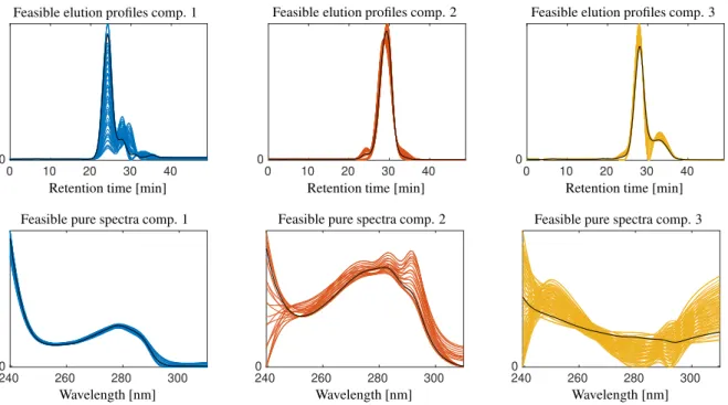
For the data sets 1 and 2 the AFS is computed by the polygon inflation algorithm [27]. Each AFS consists of three separated subsets. For this experimental data small deviations from strict nonnegativity should be allowed. The control parameters areεC =εS =7·10−3according to (5). Fig. 6 shows the concentration factor and the spectral factor AFS for data set 1 together with the true profiles by Fig. 5, namely those elution profiles with the smallest deviation from unimodal profiles and those spectra that are closest in the mean squares sense to the given spectra. These six profiles are represented by the six vertices of the two triangles.
0 10 20 30 40
0
Retention time [min]
Feasible elution profiles comp. 1
0 10 20 30 40
0
Retention time [min]
Feasible elution profiles comp. 2
0 10 20 30 40
0
Retention time [min]
Feasible elution profiles comp. 3
2400 260 280 300
Wavelength [nm]
Feasible pure spectra comp. 1
240 260 280 300
0
Wavelength [nm]
Feasible pure spectra comp. 2
240 260 280 300
0
Wavelength [nm]
Feasible pure spectra comp. 3
Figure 7: Feasible elution profiles (top) and pure component spectra (bottom) for data set 1. These profiles correspond to the AFS sets as shown in Fig. 6. The finitely many profiles in each plot correspond to the same number of the grid points of uniform grids covering the AFS subsets. No further requirements were placed on these profiles than nonnegativity. Many of the elution profiles are not unimodal and are thereby not meaningful.
Fig. 8 shows the remaining profiles under unimodality constraints. The true profiles from Fig. 5 are plotted as black lines.
The mathematical relation between points in the AFS, namely vectors of expansion coefficients, and the associated profiles is as follows: A pointx(i) = (x(i)1 ,x(i)2) ∈ MS ory(i) =(y(i)1 ,y(i)2 ) ∈ MC represents the associated (feasible) profile
s(i) =(1, x(i))VT or c(i)=UΣ(1,y(i))T.
If we cover an isolated subset of the AFS with a more or less uniform grid and plot for each node of the grid the associated profile, then we get a good approximation of the band of feasible profiles. Figure 7 shows these bands of profiles for the two AFS sets as shown in Fig. 6.
3.4.2. The AFS under unimodality constraints
Assuming elution profiles as unimodal is often well-justified and has a strong impact on the set of feasible solutions.
This is reflected in smaller bands of feasible solutions and in a smaller AFS in comparison to the non-reduced original AFS. The idea to combine unimodality assumptions with the AFS is relatively new and discussed in [48, 49].
Figure 8 shows the unimodality restricted AFS and the associated profiles for data set 1. For these computations the control parameters on nonnegativity according to Eq. (5) areεC =εS =7·10−3. The control parameterω =0.025 limits small deviations from strict unimodality, cf. Algorithm 1. The weight factors areα1 =α2 =1 andβunimodal,C= 0.1. The unimodality restrictions on the concentration factor AFS imply, by so-called duality, further restrictions on the spectral AFS; we skip the plots of this duality-based restricted spectral AFS here.
0 5 10 15 0
10 20 30 40 50 60
Concentration factor AFS & unimodality
y1
y2
20 25 30 35
0
Retention time [min]
Unimodality restricted elution profiles, comp. 1
20 25 30 35
0
Retention time [min]
Unimodality restricted elution profiles, comp. 2
20 25 30 35
0
Retention time [min]
Unimodality restricted elution profiles, comp. 3
Figure 8: Impact of the unimodality constraint on the AFS and the bands of feasible elution profiles for data set 1. Top left: Reduced AFS. The original AFS is marked by dashed lines. Other plots: The associated bands of unimodal elution profiles. The original profiles are marked in transparent colors in order to point out the effectiveness of the unimodality constraint.
3.4.3. Problems with bi-directional unimodal profiles
The AFS computation for data set 2 yields AFS sets of special structure. The concentration factor AFS and the spectral factor AFS consist of very large and narrow subsets together with others that are much smaller and close to the origin.
All this makes it difficult to construct meaningful solutions in the geometric way as explained above. We see a possible explanation in the structure ofDas shown in the left subplot of Fig. 2 where two main nonzero signal regions can be identified that are weakly coupled. Weakly coupled sub-spectra suggest to split the data set to two independent data sets and then to subject them to a separate analysis. On the one hand, this would ignore the weak coupling. On the other hand, a joint analysis of the full data set runs into the problem that the matrixDTDis close to a reducible matrix for which the AFS cannot work. In such borderline cases, it is known that the AFS can consist of long narrow subsets. A possible explanation is that unimodal profiles are to be constructed from linear combinations of singular vectors. Only the first singular vector can be unimodal, whereas the other singular vectors are typically due to their mutual orthogonality non-unimodal. The finding of unimodal linear combinations is then difficult - a circumstance which can intuitively be understood while working with the FACPACK module Duality/Complementarity & AFS on this data set; see Appendix A on the FACPACK software.
4. Results & Discussion of the chemometric analysis
Next further results on the pure component estimation for the two data sets are presented and discussed. First, we consider the pure component estimation of the problematic data set 2 under unimodality constraints for each of the two factors, see also Sec. 3.4.3. Second, we discuss the question of how to select a proper number of componentss.
Various estimations are computed and analyzed.
The results in this section demonstrate the potential of AFS techniques for analyzing ambiguous MCR outputs. We do not claim that the AFS can help for any liquid chromatography separation. However, the usefulness of AFS techniques is likely to increase with an increasing complexity and mutual overlap of the given chromatographic data.
4.1. Pure component calculation for data set 2
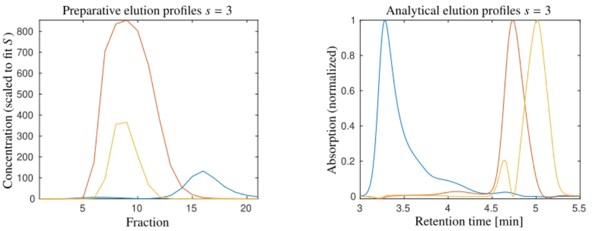
As already mentioned in the first paragraph of Sec. 3, the naming of the second factor in D = CST suggests an interpretation as a spectral factor. However, data set 2 does not include a frequency axis as all absorption measurements are taken at the fixed wavelength 280 nm. As we focus on the bilinear data structure we do not see a strong necessity for introducing a new variable name for the second factor. Unimodal profiles are expected for each factor. Within the factorization process it turned out that two observable peaks in the analytical dimension have nearly the same preparative elution profile. Hence it can be merged in a joint analytical elution profile, which is then a bi-modal profile. Thus unimodality is applied only for all but one analytical and for all preparative elution profiles. For the reconstruction of s = 3 components the information from z = 4 singular vectors is used, see [34]. The control parameters and weight factors areεC = εS = 10−4, α1 = 100, α2 = 1, βunimodal,C = 10, βunimodal,S = 50 and ω = 10−4. The considerably different sizes of the weight factors is justified by the asymmetric resolution for the chromatograms, namelyk=21 andn=3751. Additionally, the function values of the function penalizing deviations from unimodality are usually much smaller than those on deviations from nonnegativity. In order to balance these constraints, the weight factor of the unimodality constraint function is taken larger than that of the nonnegativity constraint function. Whether or not the weight factor choice is suitable can be checked by evaluation of the weighted residuals. For the given problem well-balanced values read as follows
kD−CSTk2F− X21
i=4
σ2i =1.3·10−29, α21gnonneg(C)=2.1·10−2, α22gnonneg(S)=5.0·10−2, β2unimodal,Cgunimodal(C)=7.4·10−2, β2unimodal,Sgunimodal(S)=1.4·10−3.
The results are presented in Fig. 9 for the case of selecting s = 3 main components. From the perspective of a practitioner, the species drawn in blue and red in Fig. 9 correspond to the aggregates and the product, respectively. The elution profiles are largely consistent with the results from manual data analysis shown in Fig. 5B in [30]. The species drawn in ochre was not detected during manual data analysis in [30]. It seems to correspond to a lumped component of non-ideal elution behavior of the main peak and of product fragments which tend to be obscured by the main peak.
Upon careful inspection of the analytical chromatograms in the right subplot in Fig. 2, a shoulder is distinguishable above 5 min retention time. While a manual analysis would be challenging, MCR allows to systematically extract the shoulder as additional species thus improving reproducibility.
5 10 15 20
0 100 200 300 400 500 600 700 800
Fraction
Concentration(scaledtofitS)
Preparative elution profiless=3
3 3.5 4 4.5 5 5.5
0 0.2 0.4 0.6 0.8 1
Retention time [min]
Absorption(normalized)
Analytical elution profiless=3
Figure 9: Pure component estimation for data set 2 for the case ofs=3 assumed species. Unimodal profiles are used for each factor except for one analytical elution profile drawn in ochre for which the singular value decomposition does not permit a signal separation. This compound profile includes the two peaks centered at 4.64 min and 5.01 min. For the reconstructionz=4 singular vectors are used in order to improve the results.
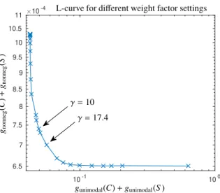
4.2. Verification of the weight factor ratios by an L-curve for data set 2
A suitable choice of the weight factors is important for the final success of the Pareto optimization of the objective function (4). Next various combinations of weight factors are tested for data set 2. Then the resulting pure component profiles are used in order to evaluate the penalty functions including their weight factors in separate form. For these computations we assumes=3 components.
Next we compare the nonnegativity constraint and the unimodality constraint. The weight factors are as follows
α1=100, α2=1, α3=1, βunimodal,C=γ, βunimodal,S=5γ. (7)
The L-curve is plotted in Fig. 10 for several valuesγ∈[0.01,500], see [37, 38] for the L-curve technique.
10-1 100 6.5
7 7.5 8 8.5 9 9.5 10 10.5
11 10-4
gunimodal(C)+gunimodal(S) gnonneg(C)+gnonneg(S)
L-curve for different weight factor settings
γ=10 γ=17.4
Figure 10: L-curve for various weight factor settings for data set 2 ands=3 components. The choiceγ=10 in (7) results in the estimation shown in Fig. 9. Values ofγthat are closer to the kink (point of highest curvature) of the L-curve asγ=17.4 result in a nearly unchanged factorization.
The total deviation iskC−Cke2F/kCk2F+kS−eSk2F/kSk2F=10−5if (C,S) correspond toγ=10 and (C,eeS) correspond toγ=17.4.
4.3. Detection of the number of components
The numbersof singular vectors that are used for the construction of the pure component factors is sometimes difficult to determine. Indicators on the size ofscan be a prior knowledge on the number of chemical species in the system or the size distribution of the singular values of the matrixD. In ideal cases the size distribution shows a clear break between a dominant set ofssingular values that are characteristically larger than the remaining set of singular values.
These latter singular values are sometimes close to zero and their origin can be seen in noise. Typical situations are illustrated by Fig. 5 in [29], Fig. 2 in [50] or Fig. 5 in [41].
The decision on a proper choice ofsis problematic for the given protein chromatographic data sets, cf. the plots of the singular values in Figs. 3 and 4. For data set 1 eithers = 3 ors =4 are reasonable values. For data set 2 the choices=3 appears to be possible for a first analysis, but this ignores many singular values that are relatively large.
The observed high number of relevant singular values was attributed to multiple sources. First of all, protein systems generally contain a large number of subspecies, i.e. product- and contaminant-isoforms. Furthermore, analytical chromatography may display deviations from ideal bilinear behavior [8]. As we try to reconstruct only the main species and neglect analytical imperfections, the SVD helps to denoise the data.
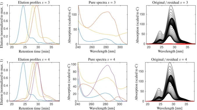
4.3.1. Pure component estimation for data set 1 with s=4species
Whenever there are doubts about the appropriate choice of the number of componentss, it is advisable to experiment with an increased or sometimes decreased s. Therefore we try a second estimation for data set 1 with s =4 com- ponents. Once again unimodality constraints are applied to the elution profiles. The results are presented in Fig. 11 together with a comparison to the results fors=3. The estimation fors=4 species is not interpretable since only the component ribonuclease A (blue) appears to be correct and the other spectral profiles cannot be associated to the other protein species. Especially the red spectrum shows pronounced deviations from the typical profile with a minimum near 280 nm instead of a maximum.
4.3.2. Pure component factorization for data set 2 and different numbers of species s
The SVD of the matrix underlying data set 2 does not clearly indicate the number of species s. We tried various combinations of the numberssandz. Unimodality constraints are used for all but one profile in the analytical elution direction and for all profiles in the preparative elution direction. The weight factors for all these experiments are listed in Sec. 4.1. Decompositions are computed fors∈ {2, . . . ,7}. The resulting minimal values of the objective function (4) are numerically evaluated. These values are plotted in Fig. 12 together with the final values of the unimodality constraint function and the relative reconstruction errors. Onlys=3 results in an interpretable solution, see Fig. 9.
For the factorization withs=2 a number ofz=4 singular vectors has been used. For all other factorizationszequals s+1.
20 25 30 35 0
0.2 0.4 0.6 0.8 1
Retention time [min]
Elution(normalizedtomax.1) Elution profiless=3
2400 260 280 300
50 100
Wavelength [nm]
Absorption(scaledtoC)
Pure spectras=3
20 25 30 35
0 50 100 150
Wavelength [nm]
Absorption(scaledtoC)
Original/residuals=3
20 25 30 35
0 0.2 0.4 0.6 0.8 1
Retention time [min]
Elution(normalizedtomax.1) Elution profiless=4
240 260 280 300
0 20 40 60 80 100
Wavelength [nm]
Absorption(scaledtoC)
Pure spectras=4
20 25 30 35
0 50 100 150
Wavelength [nm]
Absorption(scaledtoC)
Original/residuals=4
Figure 11: Pure component estimations and the residuals for data set 1 with respect tos=3 (top row and see also Fig. 5) ands=4 (lower row).
For the (s=4)-component estimation only the pure component of ribonuclease A (blue) is correct. In contrast to this, all profiles of the estimation withs=3 components can be associated with biopharmaceutical components. In the right plots the residualsD−CSTare drawn in red together with the original spectral data in black. Not surprisingly the residual is smaller for the largers=4.
2 3 4 5 6 7
10-8 10-6 10-4 10-2 100 102
f(T(opt))
kD−CSTk2F/kDk2F β2Ckgunimodal(C)k2 β2Skgunimodal(S)k2 Objective and penalty function values versuss
No. componentss
Functionvalues
Figure 12: Function values of the objective functions and of the penalty functions for pure component estimations of data set 2 versus various settings of the number of componentss. For eachs∈ {2, . . . ,7}the objective function fby (4) is optimized and the final values for the optimalT are evaluated and plotted by blue crosses. Further, the final values of the penalty function on unimodality for the preparative elution profiles are marked by red triangles. The analogous values for the analytical elution profiles are plotted by ochre squares. The weight factors areβC=10 and βS =50. Additionally, the relative reconstruction errorkD−CSTk2F/kDk2Fis shown by purple circles. However, the latter term is not part of the objective function in this form. ThereinC=UΣ(T(opt))+andST=T(opt)VTare the factors for the optimal transformationT(opt). Biochemically interpretable are only the results for the choices=3. See Fig. 9 for the resulting unimodal profiles fors=3 ands=4.
15 20 25 30 35 40 0
0.2 0.4 0.6 0.8
Elution time [min]
Conc.analytics[g/L]
Ribonuclease A
15 20 25 30 35 40
0 0.2 0.4 0.6
Elution time [min]
Conc.analytics[g/L]
Lysozyme
15 20 25 30 35 40
0 0.2 0.4 0.6 0.8
Elution time [min]
Conc.analytics[g/L]
Cytochrome c
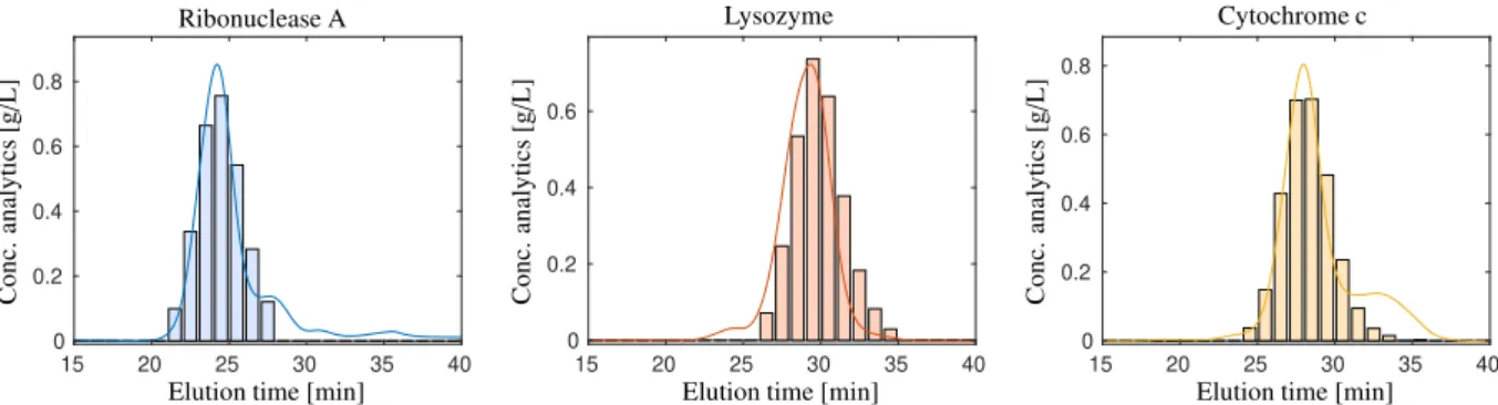
Figure 13: Comparison of the computed results (lines) and the off-line analytic (bars, measured concentrations) for data set 1. The profiles are scaled in terms of a least-squares fit compared to the offline analytic. The deviations appear to be acceptable with respect to the different measurements.
Off-line analytics results in profiles with a slight tailing. The peaks are asymmetric for higher retention times.
4.4. Verification of the results by quantitative analysis
The methodology introduced and applied in this paper results in qualitative (non-scaled) profiles. The knowledge of an underlying kinetic model, additional information of certain concentration profiles or of elution profiles (for example from separate measurements) can help to determine the correct scaling of all profiles forming the columns ofCand S. Although a quantitative analysis is not a primary focus of the suggested techniques, we carry out a quantitative analysis to check the accuracy of the results for data set 1.
Fig. 13 compares the computed profiles with off-line analytical results for data set 1. The profiles are scaled by means of a least-squares fit to offline analytical measurements (interpolation is used due to different time grids). The results are largely consistent. Minor deviations can be traced back to different recording techniques (the values of off-line analytics are averaged values). We note that the measuring sites of the off-line analytics and for recording spectroscopic dataDare different. This can result in a minor tailing of the peak profiles and a slight profile smoothing due to dispersion of the chromatographic system.
Next the root mean square error of the prediction (RMSEP), the coefficients of determination (R2values) as well as a relative error estimator∆are evaluated in order to compare the computed and the predicted profiles. These values are given by
RMS EPℓ = vt
1 n
Xn
i=1
C(i, ℓ)−C(i, ℓ)b 2
, R2ℓ =1− Pn
i=1
C(i, ℓ)−C(i, ℓ)b 2
Pn i=1
C(i, ℓ)−Ci
2 , ∆ℓ = Pn
i=1
C(i, ℓ)−C(i, ℓ)b 2
Pn i=1
C(i, ℓ)b 2
forℓ =1, . . . ,3. ThereinCare the computed profiles. FurtherCbcontains the predicted profiles and the mean values are given byCℓ = 1nPn
i=1C(i, ℓ). The profiles are interpolated for then =49 predicted grid points. Once again the profiles are scaled in terms of a least squares fit. The values are
RMS EP=(0.0373, 0.0529, 0.0380) g/L, R2=(0.946, 0.886, 0.942), ∆ =(0.045,0.092, 0.048) in the order ribonuclease A, lysozyme, cytochrome c.
4.5. Comparison with results gained by MCR-ALS
MCR-ALS is a well established MCR-toolbox for the pure component recovery from spectral mixture data, see e.g. [12, 51]. Its idea is to compute a factorization D = CST by solving iteratively least squares problems in an alternating way and where nonnegativity constraints are applied in each step. This strategy is comparable to clas- sical numerical routines to compute nonnegative matrix factorizations (NMFs), see [21]. Additional constraints as unimodality, closure or equality can also be applied. We use MCR-ALS for the computation of the factorsC and S and assume unimodality of the elution profiles (columns ofC). Next the results are compared for the data sets 1 and 2. Figure 14 shows the MCR-ALS profiles by dash-dotted lines in combination with the results gained by Pareto optimization and which are separately plotted in Figs. 5 and Fig. 9. The profiles for each of the data sets nearly co- incide. Considering the set of all feasible profiles, we would like to point out that the AFS approach is more general as it informs the user on potential ambiguities of the profiles. It gives access to all solutions that any MCR method can provide. But it is equally important to provide selection strategies to find the correct solution within the bands of feasible solutions. The present results indicate that our optimization-based selection strategy can successfully extract the correct profiles.