Analysis of the ambiguity in the determination of quantum yields from spectral data on a photoinduced isomerization
Henning Schrödera,b,∗, Cyril Ruckebuschc, Olivier Devosc, Rémi Métivierd, Mathias Sawalla, Denise Meinhardta,b, Klaus Neymeyra,b
aUniversität Rostock, Institut für Mathematik, 18057 Rostock, Germany
bLeibniz-Institut für Katalyse, 18059 Rostock, Germany
cUniv. Lille, CNRS, UMR 8516 - LASIR - Laboratoire de Spectrochimie infrarouge et Raman, 59000 Lille, France
dENS Cachan, CNRS, UMR 8531 - PPSM - Laboratoire de Photophysique et Photochimie Supramoléculaires et Macromoléculaires, 94235 Cachan Cedex, France
Abstract
Multivariate curve resolution (MCR) helps to uncover the spectra and concentration profiles of the pure components from sequences of spectra measured at a chemical reaction system. However, the underlying matrix factorization problem has often multiple solutions. This fact is known under the keyword rotational ambiguity and explains why different MCR methods can provide different decompositions for the same data. Kinetic reaction models can be used in order to constrain the feasible concentration profiles. This reduces the rotational ambiguity. Especially in the case that a first-order reaction model is assumed, the remaining ambiguity can be described completely analytically.
A hard-model based MCR method is used for the simultaneous analysis of multiple data sets. The method is tested for a reversible two-step photokinetic model. The kinetic model cannot enforce a single, unique solution. Instead the remaining ambiguity is fully investigated. The practical benefit of the method is demonstrated for an experimental UV/Vis data set of a photoinducedisomerization.
Keywords: Multivariate curve resolution, Kinetic modeling, Ambiguity of kinetic parameters, Multiset analysis.
1. Introduction
Multivariate curve resolution (MCR) techniques are highly useful for the analysis of chemical reaction systems.
Their central objective is the reliable extraction of pure component information from time series of spectra. Let D ∈ Rm×n be the row-wise matrix representation of a sequence of mspectra, each with n data channels. For an s-component chemical reaction system the aim is to determine nonnegative factorsC∈Rm×sandS ∈Rn×sso that
D=CST (1)
holds. Any pair of nonnegative matricesC andS that fulfills Equation (1) is called feasible. The occurrence of multiple nonnegative matrix pairs (C,S) satisfying (1) is paraphrased by the keywordrotational ambiguity[1, 2, 3].
An important challenge of MCR analyses is to identify those feasible factors that contain chemically meaningful information. A number of different approaches has been proposed in the literature to overcome this problem. On one hand there are optimization-based MCR methods which in combination with additional constraints yield by their construction a single pair of feasible factors. This solution is often assumed to be the true, chemically correct solution [4, 5, 6]. On the other hand there are global methods which yield the set of all feasible factorizations of D. A prominent global method is the feasible bands approach [7] that represents all feasible matrix factors in plots of the bands of all feasible spectra and concentration profiles. An alternative global approach is theArea of feasible solutions (AFS) representation [8, 9, 10, 11], which provides a low-dimensional representation of the feasible bands in terms of the expansion coefficients of the left and right singular vectors ofD.
∗Corresponding author
Kinetic reaction models can be combined with each of these techniques [2, 12, 13]. A kinetic model helps to restrict the set of feasible concentration profiles to those curves that are possible solutions of the kinetic reaction equations for optimized kinetic parameters. In general, kinetic models are well-known to be very effective in reducing the rotational ambiguity [12, 14, 15]. However, the usage of consecutive first-order reaction models is often not sufficient in order to obtain a unique solution [16, 17, 18]. See also [19] for a general approach to this problem with arbitrary first-order models. In this work, the methodology is to consider the set of all feasible factorsCandS for which a given kinetic model can be parameterized in a way that the concentration profiles are consistent with the factor C. An elegant and concise representations of these consistent factors is possible by collecting all the associated kinetic parameters within a set ofD-consistent parametersK, see [19]. This representation enables an unbiased analysis of the feasible factorizations under the constraint of a kinetic modeland reveals the underlying correlations of the kinetic parameters.
In this paper the set ofD-consistent parameters (here in the form of quantum yields)Kis derived for the reversible two-step photokinetic modelY ↔X↔Z. Therefore a hard-modeling approach is introduced which can be applied to multisets [20, 21, 22]. This enables the calculation of a pair of feasible factors, which determine an initial element in the setK. Based on this initial element, equations for the analytical description of the setK are derived. This makes it possible to evaluate the rotational ambiguity under the constraint of the given photokinetic model.
1.1. Organization of the paper
Section 2 presents a kinetic hard-modeling approach for multisets. The reversible two-step photokinetic model is analyzed in Section 3. To this end, the model is introduced, the analytical derivation of the set of D-consistent quantum yields is derived in Section 3.1 and an approximation of the photokinetic factor is presented in Section 3.2.
Finally, the results are applied to an UV/Vis multiset in Section 4.
2. Kinetic hard-modeling for multisets
The “classical” MCR analysis of an s-component system involves the extraction of concentration profiles and spectra of the pure components from a sequence ofmspectra stored in a matrix D ∈ Rm×n. Nonnegative factors C ∈ Rm×s andS ∈ Rn×s are to be determined such that (1) holds (at least approximately). The intrinsic ambiguity of this problem often requires the usage of a-priori assumptions on the factorsC and/orS, e.g. kinetic models, unimodality, monotonicity or selectivity [14]. This ambiguity can also be reduced by analyzing multiple, differing data sets of the same reaction system. Such data can be acquired by a repeated execution and measurement of the experiment under different conditions. The resulting collection of data sets can be concatenated into a so-called multiset. The higher-dimensional multiset data can be processed in a simultaneous analysis. In this section we present a modification of the kinetic hard-modeling approach from [19], which can be applied to multisets that are regularized by photokinetic models. Our approach is based on ideas from [12]. If the reader is familiar with the analysis of multisets and hard-model approaches, then the remaining part of this section can be skipped.
A common experimental setup is to vary one or several properties of a reaction system (e.g. initial concentrations, pressure, pH-value, etc.) and to measure time-dependent series of spectra under the changed conditions. This results inpdata setsD1 ∈Rm1×n, . . . ,Dp∈Rmp×nwithmi,i=1, . . . ,p, being the numbers of time points of thei-th data set andnthe number of data channels of every spectrum. The underlying assumption is that only the dynamic behavior of the species is different between the individual data sets, whereas their spectra remain unchanged. The pmatrices Diare concatenated to form the matrix
D=
D1
... Dp
∈Rmt×n (2)
withmt =m1+. . .+mp. Under the given assumption one wants to extract a common pure spectra matrixS ∈Rs×n, which fits to allDi,i=1, . . . ,p, in the sense that individual factors of concentration profilesCi∈Rmi×s,i=1, . . . ,p
exits with
D1
... Dp
|{z}
D
=
C1
... Cp
|{z}
C
ST.
Next we assume that kinetic models are known for thepdata sets of the investigated reaction system. The hard- modeling approach in [19, 12] is based on the minimization of an objective function f(φ) with the parameters of the kinetic modelφ∈Rq. This hard-modeling approach has been introduced for applications to single data sets. In the following we introduce a generalization for applications to multiple bilinear data sets. Only minor changes of f(φ) are required, which are described in detail next.
In this paper we consider the case of a photokinetic model to describe the behavior of a photoreaction in which the so-calledquantum yieldstake the place of the kinetic parameters in thermal reactions [27]. Thepphotokinetic models for the data setsD1, . . . ,Dpare defined bypinitial value problems (IVP) for ordinary differential equations (ODE).
Each IVP has an associated vector of initial concentrationsc0,i,i=1, . . . ,p. All ODE systems depend on the (same) unknown vector of quantum yieldsφfor which optimal values are to be determined. The matricesCodei (φ)∈Rm+i×s, i=1, . . . ,p, can be obtained by numerical integration of the pIVPs with respect to the given time grid. Thus these matrices represent the evaluations of thepphotokinetic models. The concatenated matrixCode(φ)∈Rm+t×sis defined by
Code(φ)=
Code1 (φ)
... Codep (φ)
.
Further letUΣVT be the truncated singular value decomposition [23] ofDwhich includes only the firstssingular values and the firstsleft and right singular vectors. The recipe for the numerical evaluation of the target function can be taken over directly from [19]. The main computation steps are as follows:
1. ComputeCode(φ) for the current quantum yieldsφ, 2. form the transformationT =(Code(φ))+UΣ,
3. compute fromT the associated factorsC=UΣT−1andST=T VT and finally 4. evaluate the function value of the objective function
f(φ)=
mt
X
i=1
Xs
j=1
min Ci j
maxl(Cl j),0
!2
| {z }
nonnegativity constraint onC
+ Xn
i=1
Xs
j=1
min Si j
maxl(Sl j),0
!2
| {z }
nonnegativity constraint onS
+kCode(φ)−Ck2F
| {z }
kinetic fit
.
(3)
Minimization algorithms as the Nelder-Mead simplex method [24] or the trust-region reflective method [25] can be used to solve the minimization problem
kf(φ)k2 → min. (4)
This procedure yields the feasible factorsC∗ and S∗ as well as an optimized vector of quantum yieldsφ∗ of the photokinetic models.
3. Ambiguity of the photokinetic parameters
This section introduces a reversible two-step kinetic model for a photoinduced reaction system. Further the set of D-consistent quantum yields is derived for this model. The photokinetic model for thes=3 componentsX,Y andZ reads
Y φ−1
GGGGGGGB F GGGGGGG
φ1
X φ2
GGGGGGB F GGGGGG
φ−2
Z (5)
with the unknown vector of quantum yieldsφ=(φ1, φ−1, φ2, φ−2)T ∈(0,1]4. The corresponding ODE system reads
˙ x(t)
˙ y(t)
˙ z(t)
=F(t)·I·M(φ)
x(t) y(t) z(t)
(6) with the coefficient matrix
M(φ)=
−φ1−φ2 φ−1 φ−2
φ1 −φ−1 0
φ2 0 −φ−2
εX 0 0
0 εY 0
0 0 εZ
(7) and concentration profilesx(t),y(t) andz(t) of the three chemical speciesX,Y andZ. The incident monochromatic photon flux is denoted byI∈R, the molar absorption coefficients areεX, εY, εZ∈R+andF(t) is the time-dependent photokinetic factor.
3.1. Set of D-consistent quantum yields
The set ofD-consistent parametersKis introduced in [19]. In brief words these are the kinetic parameter vectors whose associated ODE solutions form a factorCso thatD=CSTholds for a (not necessarily nonnegative) matrixS. Therefore the determination of the setKis not necessarily associated with an MCR factorization problem forD, but arises for any fitting of a kinetic model to a single-wavelength measurement.In the context of photokinetic reaction systems we use the conceptual extension of a setKofD-consistent quantum yields. Analogously, for each vector of quantum yieldsφ∈ K, the matrixDcan be decomposed intoCST whereinCis close to the ODE solutionCode(φ) for the given vectorφ. Thus for a givenφ∈ K the factorsCandS (should at least approximately) fulfill the equations
kD−CSTkF kDkF
=0, kC−Code(φ)kF
kCkF
=0 and kmin(C,0)kF
kCkF
=0.
The last equation guarantees the nonnegativity ofC. This equation can be ignored because nonnegativity is already been guaranteed by the second equation that guarantees thatCreproduces the (necessarily) nonnegative ODE solution Code(φ). All these error measure are considered in the approximate, numerical setup that is presented in Section 4.
The set of feasible quantum yieldsK+is a subset ofKfor which additionally the matrixS satisfies kmin(S,0)kF
kSkF
=0.
The latter condition is necessary for interpreting the columns ofS as the spectra of the pure components.
Next we present a closed-form expression (analytic representation) of the setKfor the reaction system (5) with the coefficient matrixM(φ) from (7). Let a certainφ∗ ∈ K be known. Such an initial vector of quantum yields can easily be computed by the approach presented in Section 2 or any multivariate curve result method which includes kinetic model modeling. According to the main theoretical result in [19] a vector of quantum yieldsφis in the setK if and only if all eigenvalues ofM(φ) coincide with those ofM(φ∗). The eigenvalues ofM(φ∗) are
λ1=0, λ2,3=−κ(φ∗)
2 ±1 2
q
κ(φ∗)2−4δ(φ∗) (8)
with
κ(φ∗)=εXφ∗1+εYφ∗−1+εXφ∗2+εZφ∗−2,
δ(φ∗)=εXφ∗1εZφ∗−2+εYφ∗−1εXφ∗2+εYφ∗−1εZφ∗−2. (9) For the analytical representation of the setK, allφhave to be determined which leave the eigenvaluesλ1, λ2andλ3
unchanged. The setK contains all quantum yieldsφ ∈(0,1]4which meet the following conditions (see Appendix
Appendix A for details):
−λ2≤εXφ2+εZφ−2≤ −λ3 (10)
φ2>− 1 εXεZφ−2
(εZφ−2+λ2)(εZφ−2+λ3) (11)
φ1(φ2, φ−2)=− 1 ε2Xφ2
·(εXφ2+εZφ−2+λ2)·(εXφ2+εZφ−2+λ3) (12) φ−1(φ2, φ−2)=1
εY
(κ(φ∗)−εXφ1(εXφ2, εZφ−2)−εXφ2−εZφ−2) (13) Equations (12) and (13) are explicit representations of the quantum yieldsφ1 andφ−1in dependence ofφ2 andφ−2. Together with the bounds (10) and (11) these are two explicit representations of the set of feasible quantum yieldsK. Eqns. (11)–(13) are the basis for an efficient calculation and generation of plots of the set of feasible quantum yields K.
Remark 3.1. Two correlations between the results of this section and other (photo-)kinetic models are:
a) The kinetic model(5)and the analytic representation of the setK can be reduced to a “classical” reversible two-step reaction by setting F(t)=1for all times t and I=εX =εY =εZ =1.
b) By setting the correspondingφivalues to zero, the setsKcan be derived for various models based on the Eq.
(10)-(13), e.g.
Y φ−1
GGGGGGGA X φ2
GGGGGGA Z, Y φ−1
GGGGGGGB F GGGGGGG
φ1
X φ2
GGGGGGA Z and Y φ−1
GGGGGGGA X φ2
GGGGGGB F GGGGGG
φ−2
Z.
Relabelling of the components and quantum yields/rate constants might be necessary to meet common notation standards.See [19] for more details on the three models above.
3.2. Approximation of the photokinetic factor
The functionF(t) in (6) is not known in advance and must therefore be approximated. Photoinduced reactions are triggered by light at a chosen irradiation wavelengthλ(405 nm here). If we denote bydλ(t) the absorption of the reaction system at the wavelengthλalong the time axist, then thephotokinetic factorcan be approximatedin a general wayaccording to
F(t)≈F(t)¯ = 1−10−dλ(t)
dλ(t) ; (14)
see Chapter 1, Equation (1.39), in [26]. A continuous evaluation of ¯F(t) is needed for the numerical integration of the IVPs of Section 2. Because of the discrete structure of spectroscopic data, two minor problems arise. First, the intensity profiledλ(t) is usually neither known for the irradiation wavelengthλnor for continuous time pointst. The column ofDthat corresponds to the wavelength which is nearest toλcan be used to approximatedλ(t) on the given time grid. Second, the values ¯F(t) are not obtainable for arbitrary time pointstwithin the boundaries of the time grid, but can be approximated by (linear or higher order) interpolation.
4. Numerical results
A photochromic UV/Vis study of cis-1,2-dicyano-1,2-bis(2,4,5-trimethyl-3-thienyl)ethene (CMTE) [22, 27] is investigated in this section. The reaction system containss=3 independent components, namely different forms of CMTE:X =opencisisomer,Y =closed ring form andZ =opentransisomer. The hard-modeling approach from Section 2 is applied and the setsK andK+are derived. Finally, an improved solution (by means of typical error measures) is identified inK+.
Two UV/Vis data sets D1 ∈ R103×621 andD2 ∈ R146×621 with 621 data channels in each of the 103 and 146 measured spectra are considered. They are shown in Fig. 1. The vectorx∈ R621contains the wavelength grid and is valid for both data sets. The two data sets differ in their initial concentrationsc0,1 =(5.93·10−5,0,0) mol/l and c0,2 =(0,0,1.072·10−4) mol/l as well as their incident monochromatic photon fluxesI1 =4.8·10−6 mol/(l·s) and I2=4.5·10−6mol/(l·s). Both were irradiated at the same wavelength of 405 nm and the molar absorption coefficients of the different forms at this wavelength areεX =3.1075·103, εY =1.0862·103, εZ=2.3365·103in l/(mol·cm).
6
0
300 400 500 600 0
0.5 1 1.5
wavelength [nm]
time [min]
Data setD1
absorption
12
6 0
300 400 500 600 0
0.5 1 1.5
wavelength [nm]
time [min]
absorption
Data setD2
0 300
400 0.5
500 0 1
600 0
1.5
wavelength [nm]
absorption
Concatenated data setD
time [min]
Figure 1: On the left the data setD1and in the middle the data setD2are shown. The matrixDis the result of merging the data setsD1andD2as in Equation (2) and is presented in the right plot.
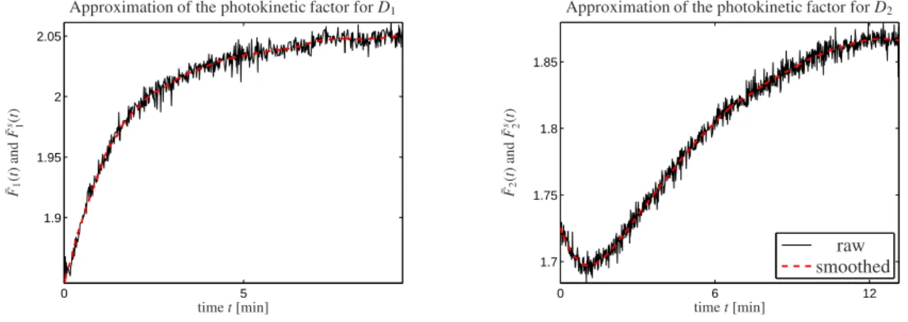
Before applying the hard-modeling approach from Section 2, approximations of the photokinetic factorsF1(t) andF2(t) have to be determined for D1 andD2. The 269thcomponent of xreads 404.98nm and is nearest to the value of the irradiation wavelengthλ=405nm. The evaluation of (14) is done for the time discrete intensity profiles D1(:,269),D2(:,269) and reads ¯F1 ∈ R103 and ¯F2 ∈ R146. Additionally, a Savitzky-Golay filter with 3rd degree polynomials and a window width of 35 points has proven to be suitable in order to reduce the influence of noise. The resulting vectors are called ¯F1s ∈ R103 and ¯F2s ∈ R146. Fig. 2 shows the raw and smoothed approximations of the photokinetic factors.
0 5
1.9 1.95 2 2.05
Approximation of the photokinetic factor forD1
timet[min]
¯F1(t)and¯Fs 1(t)
0 6 12
1.7 1.75 1.8 1.85
timet[min]
raw smoothed Approximation of the photokinetic factor forD2
¯F2(t)and¯Fs 2(t)
Figure 2: The approximations ¯F1and ¯F2of the photokinetic factors determined by Equation (14) are plotted in black. The smoothed approximations F¯s1and ¯F2swere obtained by a Savitzky-Golay filter and are shown as red dashed lines.
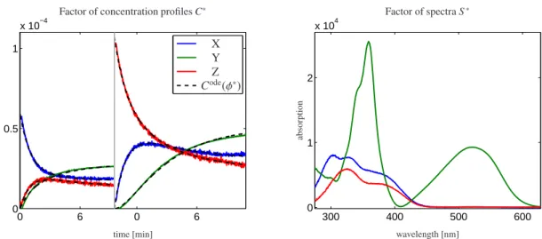
Next, the hard-modeling approach from Section 2 is used to calculate a decomposition which is consistent with the given photokinetic model (5). A solution to the minimization problem (4) is computed with the solverlsqnonlinfrom MatLab2017b. The calculated quantum yields areφ∗ = (0.1429,0.2491,0.2219,0.3678)T and the corresponding factorsC∗andS∗are shown in Fig. 3. The obtained relative errors are
kD−C∗(S∗)TkF kDkF
=0.010, kC∗−Code(φ∗)kF kC∗kF
=0.022, kmin(C∗,0)kF kC∗kF
=0.0012, kmin(S∗,0)kF kS∗kF
=0.00052.
Because of the noisy/perturbed spectral data these error values do not exactly equal 0. Therefore the setsK andK+
also contain quantum yields for which the corresponding factors have comparably small relative errors.
0 6 0 6 0
0.5 1
x 10−4
Factor of concentration profilesC∗
time [min]
concentration
X Y Z Code(φ∗)
300 400 500 600
0 1 2
x 104
Factor of spectraS∗
wavelength [nm]
absorption
Figure 3: Decomposition of the merged matrixDfrom Fig. 1; On the left the concentration profilesC∗are shown in color together with the kinetic modelCode(φ∗) as black dashed lines. The corresponding spectral profilesS∗are shown on the right. They are valid for both data setsD1andD2.
0.3 0.6 0
0.5 0.3
0.2
0.1 0.4
Set ofD-consistent parametersK
φ1
φ2
φ−2
0.3 0.6 0
0.5 0.3
0.2
0.1 0.4
φ1
φ2
φ−2
Set of feasible parametersK+
Figure 4: Representation of the setsK(left) andK+(right); The set of representatives ofKis shown as colored points in the left plot and is obtained by the use of the Equations (10)-(13). Because of noisy data the nonnegativity constraint of the factorSforK+has been applied with a tolerance of 2%. This results in the blue colored subsetK+ofKin the right plot. The quantum yieldsφ∗are marked by a black cross andφoptby a red cross in each plot.
Next the analytical description of the setKfor the photokinetic model (5) from Section 3 is used. The initial values κ(φ∗)=2263.51 andδ(φ∗)=800718.27 are first computed. Thus the eigenvalues ofM(φ∗) areλ1=0, λ2 =−438.83 andλ3 =−1824.68. An evaluation ofφ1(φ2, φ−2) from Equation (12) is done for values in the (φ2, φ−2)-plane. Only those values have to be considered for which the constraints from Equation (10) and (11) hold. The corresponding values forφ−1(φ2, φ−2) are given by Equation (13). They can be neglected in order to reduce the dimension which is needed to displayK. The left plot of Fig. 4 shows an approximation of the setK by a set of representatives. The quantum yield vectorφ∗∈ Kis used to computeκ,δand thus alsoK. It is marked by a black cross.
The second step is a reduction ofKtoK+. To this end the factorS is calculated for each representative ofKin a way that the objective function (3) is minimized. If
|min(S(i,:),0)| ≤0.02·max(S(i,:)) (15)
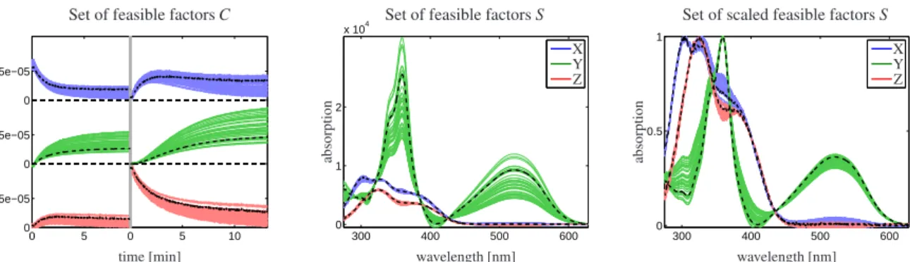
holds,then the scaled factorS (in way that all columns have a maximum of 1) contains no entry below−0.02. In other words, this strategy amounts to the acceptance of 2% negative entries inS. In conclusion the corresponding representative inKalso belongs toK+, if (15) holds fori=1, . . . ,s.The result is shown in blue color in the right plot of Fig. 4. Both setsK andK+are consistent with the approximations calculated using the grid search algorithm in
0 5 0 5 10 0
5e−05 0 5e−05 0 5e−05
Set of feasible factorsC
time [min]
concentration
300 400 500 600
0 1 2
x 104
Set of feasible factorsS
wavelength [nm]
absorption
X Y Z
300 400 500 600
0 0.5 1
wavelength [nm]
absorption
X Y Z Set of scaled feasible factorsS
Figure 5: The factorsC(left) andS (center) are shown for each representative ofK+in Fig. 4. Qualitative and quantitative differences can be observed for all species. The two plots can be interpreted as representation of the rotational ambiguity constrained by a kinetic model. A scaling to a maximal height of 1 for each spectrum is used in the right plot. This highlights that most of the feasible factorsS contain a similar structural information. Nevertheless the corresponding factorsCshow major differences. It should be noted that not only bands of solutions are shown, but a set of individual feasible factors. To emphasize this the factorsCoptandSoptforφoptare plotted by black dashed lines.
[27]. The associated bands corresponding to these feasible factorsCandS are plotted in Fig. 5. These plots constitute graphical evaluations of the rotational ambiguity of a data set under the constraint of a kinetic model. In the left and the center plot we use a scaling that is determined by the kinetic model. Consequently, scalar multiples of the same concentration profile or spectrum also appear in the plots. For better graphical evaluation of the rotational ambiguity a max-height-of-1 scaling is used in the right plot.
Next, the correctness of the setK+is validated. Therefore, the nonnegativity and the fit to the kinetic model is evaluated for all the representatives ofK+as plotted in Fig. 4. Table 1 contains the relative errors forφ∗as reference values as well as the corresponding lower and upper bounds. The relative error is between 0.0009 and 0.015 for the
kC−Code(φ)kF/kCkF kmin(C,0)kF/kCkF kmin(S,0)kF/kSkF
φ=φ∗ 0.022 1.2 E−3 5.2 E−4
Upper bound for allφ∈ K+ 0.067 1.5 E−2 9.8 E−3
Lower bound for allφ∈ K+ 0.020 9.0 E−4 4.0 E−4
φ=φopt 0.021 1.1 E−3 5.1 E−4
Table 1: The relative errors of the corresponding factors for the vector of quantum yieldsφ∗andφoptas well as lower and upper bounds are listed.
nonnegativity ofC and between 0.0004 and 0.0098 for the nonnegativity ofS. This is considered to be sufficiently good. The relative error for the kinetic fit ranges between 0.02 and 0.067. The relatively large upper limit is caused by the noise contained inD1andD2, which is mainly found in the concentration factors (compare the left and right plot in Fig. 3).
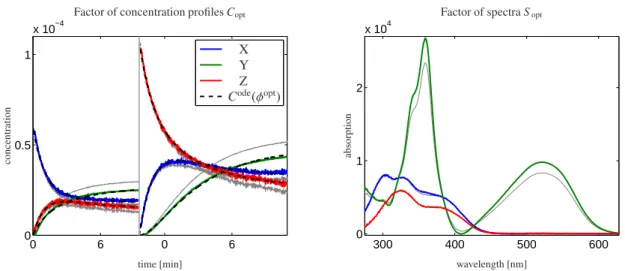
In the final step of the analysis the representatives of the setKare scanned for a vector of quantum yields which results in smaller error values compared to that which belong toφ∗. The optimal vector of quantum yields reads φopt =(0.1355,0.2592,0.2263,0.3671). Its relative error values are listed in the last row of Table 1. Optimality is to be understood in the sense of smallest error values. This does not necessarily include that the found solution has the greatest chemical meaning. Nevertheless, these two interpretations are often correlated. The optimal vector is marked by a red cross in Fig. 4. The two vectorsφ∗andφopt differ only slightly. A graphical comparison of corresponding factorsCopt,Sopt(colored) withC∗,S∗(gray) is given in Fig. 6. While the spectra of the componentsXandZremain nearly unchanged, a clear difference can be seen for the spectrum of the second componentY. Additionally, the concentration profiles show major differences in all components. Hence the small difference betweenφ∗andφoptcan yield qualitatively different but still feasible solutions.
5. Conclusion
Kinetic models can support MCR methods in reducing the rotational ambiguity of pure component factorizations for bilinear data. However, even under the constraint of the consistence to a kinetic hard model, a unique factorization
0 6 0 6 0
0.5 1
x 10−4
Factor of concentration profilesCopt
time [min]
concentration
X Y Z Code(φopt)
300 400 500 600
0 1 2
x 104
Factor of spectraSopt
wavelength [nm]
absorption
Figure 6: Decomposition of the merged matrixDfrom Fig. 1; On the left the concentration profilesCoptare shown in color together with the kinetic model solutionCode(φopt) by black dashed lines. The corresponding spectral profilesSoptare shown on the right. The factorsC∗andS∗are also plotted in gray for comparison purposes.
cannot always be guarantied.
In this paper we have demonstrated a mathematical analysis which allows us to investigate the remaining am- biguity of a kinetic-hard-model based MCR approach. The ambiguity is presented in closed-form mathematical expressions for the quantum yield vectors of a reversible two-step photochemical system that are consistent with the spectroscopic data.
We hope that the presented strategy on the hand can raise awareness for MCR-ambiguities even under the kinetic- hard-model conditions and on the other hand can highlight the strength of the mathematical-analytic representation of the set of feasible quantum yields.
Appendix A. Equations for the analytical description ofK
This section contains the mathematical derivation of the Equations (10)-(13) that describe the setKfor the kinetic model (5). We assume that the two eigenvaluesλ2andλ3in Equation (8) are enumerated in a way that 0> λ2> λ3. The two sets
M:=
(
φ∈(0,1]4 : λ2,3=−κ(φ) 2 ±1
2 q
κ(φ)2−4δ(φ) )
, N:=n
φ∈(0,1]4 : Eq. (10)-(13) holdo
are to be considered withκ(φ) andδ(φ) by (9). It has to be shown thatM=N or equivalently thatφ∈ Mif and only ifφ∈ N.
First we prove thatφ∈ Mimplies thatφ∈ N. In a preparation step we show that the following term equals 0:
(εXφ2+εZφ−2)2−(εXφ1+εXφ2+εZφ−2)(εXφ2+εZφ−2)+εXφ1εZφ−2+εXφ1εXφ2 (A.1)
=(εXφ2+εZφ−2)2−(εXφ1−εXφ1
| {z }
=0
+εXφ2+εZφ−2)(εXφ2+εZφ−2)
=(εXφ2+εZφ−2)2−(εXφ2+εZφ−2)2
=0.
Next we subtract the termεXφ1εXφ2from (A.1) and divide the equation byε2Xφ2. This results in φ1(φ2, φ−2)=− 1
ε2Xφ2
·((εXφ2+εZφ−2)2−(εXφ1+εXφ2+εZφ−2)(εXφ2+εZφ−2)+εXφ1εZφ−2)
=− 1 ε2Xφ2
·((εXφ2+εZφ−2)2−(εXφ1+εXφ−1−εXφ−1
| {z }
=0
+εXφ2+εZφ−2)(εXφ2+εZφ−2)+εXφ1εZφ−2)
=− 1 ε2Xφ2
·((εXφ2+εZφ−2)2− κ(φ)
|{z}
=−(λ2+λ3)
(εXφ2+εZφ−2)+δ(φ))
|{z}
=λ2λ3
=− 1 ε2Xφ2
·((εXφ2+εZφ−2)2+(εXφ2+εZφ−2)(λ2+λ3)+λ2λ3)
=− 1 ε2Xφ2
·(εXφ2+εZφ−2+λ2)·(εXφ2+εZφ−2+λ3).
This shows that Equation (12) holds. Equation (13) follows directly from the fact thatκ(φ)=−(λ2+λ3) is constant for allφ∈ Mso thatκ(φ)=κ(φ∗).
The nonnegativity ofφ1(φ2, φ−2) and the representation by Equation (12) imply that (εXφ2+εZφ−2+λ2)·(εXφ2+εZφ−2+λ3)<0.
Due toλ3< λ2 <0 the latter inequality can only hold ifεXφ2+εZφ−2+λ2is positive andεXφ2+εZφ−2+λ3is negative.
This proves (10).
Next the equation
(εZφ−2+λ2)(εZφ−2+λ3)=(εZφ−2)2+εZφ−2(λ2+λ3
| {z }
−κ
)+λ2λ3
|{z}
δ
= εXφ2εZφ−2+εXφ2εYφ−1=εXφ2(εZφ−2+εYφ−1) holds and hence we get
φ2>0>− εXφ2
εXεZφ−2
(εZφ−2+εYφ−1)
| {z }
>0
=− 1 εXεZφ−2
(εZφ−2+λ2)(εZφ−2+λ3).
Thus (11) holds.
Finally we show the reverse direction, namely thatφ ∈ N implies that φ ∈ M. We only have to show that κ(φ)=κ(φ∗) andδ(φ)=δ(φ∗). With (8) this proves thatM(φ) has the same eigenvalues asM(φ∗) which completes the proof.
First,κ(φ)=κ(φ∗) results from a simple reorganization of Eq. (13). Second, starting from (12) the equation φ1(φ2, φ−2)=− 1
ε2Xφ2
·(εXφ2+εZφ−2+λ2)·(εXφ2+εZφ−2+λ3)
=− 1 ε2Xφ2
·((εXφ2+εZφ−2)2+(εXφ2+εZφ−2) (λ2+λ3)
| {z }
−κ(φ∗)
+λ2λ3)
|{z}
δ(φ∗)
=− 1 ε2Xφ2
·((εXφ2+εZφ−2)2−κ(φ)(εXφ2+εZφ−2)+δ(φ∗)) follows. Multiplication byε2Xφ2and subtraction ofε2Xφ2φ1(φ2, φ−2) gives
0=−((εXφ2+εZφ−2)2−κ(φ)(εXφ2+εZφ−2)+δ(φ∗))−ε2Xφ2φ1(φ2, φ−2). (A.2) Expansion of the quadratic term and substitution ofκ(φ) by its definition reduces (A.2) to
0=εXφ1εZφ−2+εYφ−1εXφ2+εYφ−1εZφ−2−δ(φ∗))=δ(φ)−δ(φ∗).
Henceδ(φ)=δ(φ∗) has been proved.
References
[1] E. Malinowski.Factor analysis in chemistry. Wiley, New York, 2002.
[2] M. Maeder and Y.M. Neuhold.Practical data analysis in chemistry. Elsevier, Amsterdam, 2007.
[3] H. Abdollahi and R. Tauler. Uniqueness and rotation ambiguities in multivariate curve resolution methods. Chemom. Intell. Lab. Syst., 108(2):100–111, 2011.
[4] J. Jaumot, R. Gargallo, A. de Juan, and R. Tauler. A graphical user-friendly interface for MCR-ALS: a new tool for multivariate curve resolution in MATLAB.Chemom. Intell. Lab. Syst., 76(1):101–110, 2005.
[5] H. Kim and H. Park. Nonnegative matrix factorization based on alternating nonnegativity constrained least squares and active set method.
SIAM J. Matrix Anal. Appl., 30:713–730, 2008.
[6] J. Jaumot, A. de Juan, and R. Tauler. MCR-ALS GUI 2.0: new features and applications.Chemom. Intell. Lab. Syst., 140:1–12, 2015.
[7] R. Tauler. Calculation of maximum and minimum band boundaries of feasible solutions for species profiles obtained by multivariate curve resolution.J. Chemom., 15(8):627–646, 2001.
[8] O.S. Borgen and B.R. Kowalski. An extension of the multivariate component-resolution method to three components. Anal. Chim. Acta, 174:1–26, 1985.
[9] R. Rajkó and K. István. Analytical solution for determining feasible regions of self-modeling curve resolution (SMCR) method based on computational geometry.J. Chemom., 19(8):448–463, 2005.
[10] M. Sawall, C. Kubis, D. Selent, A. Börner, and K. Neymeyr. A fast polygon inflation algorithm to compute the area of feasible solutions for three-component systems. I: Concepts and applications.J. Chemom., 27:106–116, 2013.
[11] A. Jürß, M. Sawall, and K. Neymeyr. On generalized Borgen plots. I: From convex to affine combinations and applications to spectral data.
J. Chemom., 29(7):420–433, 2015.
[12] A. de Juan, M. Maeder, M. Martínez, and R. Tauler. Combining hard and soft-modelling to solve kinetic problems. Chemom. Intell. Lab.
Syst., 54:123–141, 2000.
[13] M. Sawall, A. Börner, C. Kubis, D. Selent, R. Ludwig, and K. Neymeyr. Model-free multivariate curve resolution combined with model-based kinetics: Algorithm and applications. J. Chemom., 26:538–548, 2012.
[14] N. Mouton, A. de Juan, M. Sliwa, and C. Ruckebusch. Hybrid hard- and soft-modeling approach for the resolution of convoluted femtosecond spectrokinetic data.Chemom. Intell. Lab. Syst., 105(1):74 – 82, 2011.
[15] H. Schröder, M. Sawall, C. Kubis, D. Jürß, A. Selent, A. Brächer, A. Börner, R. Franke, and K. Neymeyr. Comparative multivariate curve resolution study in the area of feasible solutions.Chemom. Intell. Lab. Syst., 163:55–63, 2017.
[16] N.W. Alcock, D.J. Benton, and P. Moore. Kinetics of Series First-Order Reactions.Trans. Faraday Soc., 66:2210–2213, 1970.
[17] S. Vajda and H. Rabitz. Identifiability and distinguishability of first-order reaction systems.J. Phys. Chem., 92(3):701–707, 1988.
[18] J. Jaumot, P. J. Gemperline, and A. Stang. Non-negativity constraints for elimination of multiple solutions in fitting of multivariate kinetic models to spectroscopic data.J. Chemom., 19(2):97–106, 2005.
[19] H. Schröder, M. Sawall, C. Kubis, D. Selent, D. Hess, R. Franke, A. Börner, and K. Neymeyr. On the ambiguity of the reaction rate constants in multivariate curve resolution for reversible first-order reaction systems.Anal. Chim. Acta, 927:21–34, 2016.
[20] R. Tauler, A. Smilde, and B. Kowalski. Selectivity, local rank, three-way data analysis and ambiguity in multivariate curve resolution.Journal Chemom., 9(1):31–58, 1995.
[21] L. Blanchet, C. Ruckebusch, A. Mezzetti, J. P. Huvenne, and A. de Juan. Monitoring and interpretation of photoinduced biochemical processes by rapid-scan ftir difference spectroscopy and hybrid hard and soft modeling.J. Phys. Chem. B, 113(17):6031–6040, 2009. PMID: 19385692.
[22] O. Devos, S. Aloise, M. Sliwa, R. Métivier, J.-P. Placial, and C. Ruckebusch. Chapter 11 - multivariate curve resolution of (ultra)fast photoinduced process spectroscopy data. In Cyril Ruckebusch, editor,Resolving Spectral Mixtures, volume 30 ofData Handling in Science and Technology, pages 353 – 379. Elsevier, 2016.
[23] G.H. Golub and C.F. Van Loan.Matrix Computations. Johns Hopkins Studies in the Mathematical Sciences. Johns Hopkins University Press, Baltimore, MD, 2012.
[24] J. C. Lagarias, J. A. Reeds, M. H. Wright, and P. E. Wright. Convergence properties of the nelder-mead simplex method in low dimensions.
SIAM J. Optim., 9(1):112–147, 1998.
[25] T. F. Coleman and Y. Li. An interior trust region approach for nonlinear minimization subject to bounds. SIAM J. Optim., 6(2):418–445, 1996.
[26] H. Mauser and G. Gauglitz.Photokinetics: theoretical fundamentals and applications, volume 36. Elsevier, 1998.
[27] O. Devos, H. Schröder, M. Sliwa, J.P. Placial, K. Neymeyr, R. Metivier, and C. Ruckebusch. Photochemical multivariate curve resolution models for the investigation of photochromic systems under continuous irradiation.Accepted by Anal. Chim. Acta, 2018.