The Physics of Quantum Mechanics

The Physics of Quantum Mechanics

James Binney

and

David Skinner

Copyright c2008–210 James Binney and David Skinner Published by Capella Archive 2008; revised printings 2009, 2010

Contents

Preface

1 Probability and probability amplitudes

1.1 The laws of probability 3

•Expectation values 4

1.2 Probability amplitudes 5

•Two-slit interference 6 • Matter waves? 7

1.3 Quantum states 7

•Quantum amplitudes and measurements 7

⊲Complete sets of amplitudes 8 •Dirac notation 8

•Vector spaces and their adjoints 9 • The energy rep- resentation 11 •Orientation of a spin-half particle 12

•Polarisation of photons 13

1.4 Measurement 15

Problems 15

2 Operators, measurement and time evolution

2.1 Operators 17

⊲Functions of operators 20 ⊲ Commutators 20

2.2 Evolution in time 21

•Evolution of expectation values 23

2.3 The position representation 24

•Hamiltonian of a particle 26 • Wavefunction for well defined momentum 27 ⊲ The uncertainty principle 28

•Dynamics of a free particle 29 •Back to two-slit in- terference 31 • Generalisation to three dimensions 31

⊲Probability current 32 ⊲ The virial theorem 33

Problems 34

3 Harmonic oscillators and magnetic fields

3.2 Dynamics of oscillators 41

•Anharmonic oscillators 42

3.3 Motion in a magnetic field 45

•Gauge transformations 46 • Landau Levels 47

⊲Displacement of the gyrocentre 49 • Aharonov-Bohm ef- fect 51

Problems 52

4 Transformations & Observables

4.1 Transforming kets 57

•Translating kets 58 •Continuous transformations

and generators 59 • The rotation operator 61

•Discrete transformations 61

4.2 Transformations of operators 63

4.3 Symmetries and conservation laws 67

4.4 The Heisenberg picture 68

4.5 What is the essence of quantum mechanics? 70

Problems 71

5 Motion in step potentials

5.1 Square potential well 74

•Limiting cases 76 ⊲ (a) Infinitely deep well 76

⊲(b) Infinitely narrow well 77

5.2 A pair of square wells 78

•Ammonia 80 ⊲ The ammonia maser 81

5.3 Scattering of free particles 83

⊲The scattering cross section 85 •Tunnelling through a potential barrier 86 • Scattering by a classically allowed region 87 • Resonant scattering 89 ⊲ The Breit–Wigner cross section 91

5.4 How applicable are our results? 94

5.5 What we have learnt 96

Problems 97

6 Composite systems

6.1 Composite systems 103

•Collapse of the wavefunction 106 • Operators for com- posite systems 107 • Development of entanglement 108

•Einstein–Podolski–Rosen experiment 109

⊲Bell’s inequality 111

6.2 Quantum computing 114

6.3 The density operator 119

•Reduced density operators 123 • Shannon entropy 125

6.4 Thermodynamics 127

6.5 Measurement 130

Problems 133

7 Angular Momentum

7.1 Eigenvalues ofJz andJ² 137

•Rotation spectra of diatomic molecules 140

7.2 Orbital angular momentum 142

•Las the generator of circular translations 144 •Spectra ofL² andLz145 •Orbital angular momentum eigenfunc- tions 145 • Orbital angular momentum and parity 149

•Orbital angular momentum and kinetic energy 149

•Legendre polynomials 151

7.3 Three-dimensional harmonic oscillator 152

7.4 Spin angular momentum 156

•Spin and orientation 157 •Spin-half systems 158 ⊲The Stern–Gerlach experiment 159 • Spin-one systems 161

•The classical limit 163 •Precession in a magnetic field 165

7.5 Addition of angular momenta 167

•Case of two spin-half systems 170 • Case of spin one and spin half 172 • The classical limit 172

Problems 173

Contents vii

8 Hydrogen

8.1 Gross structure of hydrogen 178

•Emission-line spectra 181 •Radial eigenfunctions 182

•Shielding 186 •Expectation values forr^−k 188

8.2 Fine structure and beyond 189

•Spin-orbit coupling 189 • Hyperfine structure 193

Problems 194

9 Perturbation theory

9.1 Time-independent perturbations 197

•Quadratic Stark effect 199 • Linear Stark effect and degenerate perturbation theory 200 • Effect of an ex- ternal magnetic field 202 ⊲ Paschen–Back effect 204

⊲Zeeman effect 204

9.2 Variational principle 206

9.3 Time-dependent perturbation theory 207

•Fermi golden rule 208 •Radiative transition rates 209

•Selection rules 212

Problems 214

10 Helium and the periodic table

10.1 Identical particles 218

⊲Generalisation to the case ofN identical particles 219

•Pauli exclusion principle 219 •Electron pairs 221

10.2 Gross structure of helium 222

•Gross structure from perturbation theory 223

•Application of the variational principle to he- lium 224 •Excited states of helium 225

•Electronic configurations and spectroscopic terms 228

⊲Spectrum of helium 229

10.3 The periodic table 229

•From lithium to argon 229 •The fourth and fifth peri- ods 233

Problems 234

11 Adiabatic principle

11.1 Derivation of the adiabatic principle 237 11.2 Application to kinetic theory 238 11.3 Application to thermodynamics 240 11.4 The compressibility of condensed matter 241

11.5 Covalent bonding 242

•A model of a covalent bond 242 •Molecular dynamics 244

•Dissociation of molecules 245

11.6 The WKBJ approximation 245

Problems 247

12 Scattering Theory

12.1 The scattering operator 249

•Perturbative treatment of the scattering operator 251

12.2 The S-matrix 253

•Theiǫprescription 253 •Expanding the S-matrix 255

•The scattering amplitude 257

12.3 Cross-sections and scattering experiments 259

•The optical theorem 261

12.4 Scattering electrons off hydrogen 263

12.5 Partial wave expansions 265

•Scattering at low energy 268

12.6 Resonant scattering 270

•Breit–Wigner resonances 272 • Radioactive decay 272

Problems 274

Appendices

A Cartesian tensors 277

B Fourier series and transforms 279

C Operators in classical statistical mechanics 280

D Lorentz covariant equations 282

E Thomas precession 284

F Matrix elements for a dipole-dipole interaction 286

G Selection rule forj 287

H Restrictions on scattering potentials 288

Index

Preface

This book grew out of classes given for many years to the second-year un- dergraduates of Merton College, Oxford. The University lectures that the students were attending in parallel were restricted to the wave-mechanical methods introduced by Schr¨odinger, with a very strong emphasis on the time-independent Schr¨odinger equation. The classes had two main aims: to introduce more wide-ranging concepts associated especially with Dirac and Feynman, and to give the students a better understanding of the physical implications of quantum mechanics as a description of how systems great and small evolve in time.

While it is important to stress the revolutionary aspects of quantum mechanics, it is no less important to understand that classical mechanics is just an approximation to quantum mechanics. Traditional introductions to quantum mechanics tend to neglect this task and leave students with two independent worlds, classical and quantum. At every stage we try to explain how classical physics emerges from quantum results. This exercise helps students to extend to the quantum regime the intuitive understanding they have developed in the classical world. This extension both takes much of the mystery from quantum results, and enables students to check their results for common sense and consistency with what they already know.

A key to understanding the quantum–classical connection is the study of the evolution in time of quantum systems. Traditional texts stress instead the recovery of stationary states, which do not evolve. We want students to understand that the world is full of change – that dynamicsexists– precisely because the energies of real systems are always uncertain, so a real system is never in a stationary state; stationary states are useful mathematical abstrac- tions but are not physically realisable. We try to avoid confusion between the real physical novelty in quantum mechanics and the particular way in which it is convenient to solve its governing equation, the time-dependent Schr¨odinger equation.

Quantum mechanics emerged from efforts to understand atoms, so it is natural that atomic physics looms large in traditional courses. However, atoms are complex systems in which tens of particles interact strongly with each other at relativistic speeds. We believe it is a mistake to plunge too soon into this complex field. We cover atoms only in so far as we can proceed with a reasonable degree of rigour. This includes hydrogen and helium in some detail (including a proper treatment of Thomas precession), and a qualitative sketch of the periodic table. But is excludes traditional topics such as spin–orbit coupling schemes in many-electron atoms and the physical interpretation of atomic spectra.

We devote a chapter to the adiabatic principle, which opens up a won- derfully rich range of phenomena to quantitative investigation. We also de- vote a chapter to scattering theory, which is both an important practical application of quantum mechanics, and a field that raises some interesting conceptual issues about how we compute results in quantum mechanics.

When one sits down to solve a problem in physics, it’s vital to identify the optimum coordinate system for the job – a problem that is intractable in the coordinate system that first comes to mind, may be trivial in another system. Dirac’s notation makes it possible to think about physical problems in a coordinate-free way, and makes it straightforward to move to the chosen coordinate system once that has been identified. Moreover, Dirac’s notation brings into sharp focus the still mysterious concept of a probability ampli- tude. Hence, it is important to introduce Dirac’s notation from the outset, and to use it for an extensive discussion of probability amplitudes and why they lead to qualitatively new phenomena.

The book formed the basis for lecture courses delivered in the academic years 2008/9 and 2009/10. At the end of each year the text was revised in light of feedback from both students and tutors, and insights gained whilst teaching. After the first set of lectures it was clear that students needed to be given more time to come to terms with quantum amplitudes and Dirac notation. To this end some work on spin-half systems and polarised light was added to Chapter 1. The students found orbital angular momentum hard, and the way this is handled in what is now Chapter 7 was changed. A section on the Heisenberg picture was added to Chapter 4. Chapter 10 was revised to correct a widespread misunderstanding about the singlet-triplet splitting in helium, and Chapter 11 was revised to add thermodynamics to the applications of the adiabatic principle.

The major change between the first and second printings was a new Chapter 6 on composite systems. This covers topics such as entanglement, Bell inequalities, quantum computing and density operators that are not normally included in a first course on quantum mechanics. The discussion in this chapter of the measurement problem was rewritten at the second revision. We hope it now makes clear that quantum mechanics does not form a complete physical theory, and that it will inspire students to think how it could be completed. It is most unusual for the sixth chapter of a second-year physics textbook to be able to take students to the frontier of human understanding, as this chapter does.

The major change between the second and third printings was reworking of§5.3 on one-dimensional scattering – this section now emphasises the roles of parity and phase shifts and includes resonant scattering and the Breit–

Wigner cross section.

Students encountered considerable difficulty understanding the connec- tion between spin and the gross structure of helium, so the treatment of this topic was rewritten at the second revision.

Problem solving is the key to learning physics and most chapters are followed by a long list of problems. These lists have been extensively revised since the first edition and printed solutions prepared. The solutions to starred problems, which are mostly more-challenging problems, are now available online¹ and solutions to other problems are available to colleagues who are teaching a course from the book. In nearly every problem a student will either prove a useful result or deepen his/her understanding of quantum mechanics and what it says about the material world. Even after successfully solving a problem we suspect students will find it instructive and thought-provoking to study the solution posted on the web.

We are grateful to several colleagues for comments on the first two editions, particularly Justin Wark for alerting us to the problem with the singlet-triplet splitting. Fabian Essler, John March-Russell and Laszlo Soly- mar made several constructive suggestions. We thank our fellow Mertonian Artur Ekert for stimulating discussions of material covered in Chapter 6 and for reading that chapter in draft form.

July 2010 James Binney

David Skinner

1http://www-thphys.physics.ox.ac.uk/users/JamesBinney/QBhome.htm

1

Probability and probability amplitudes

The future is always uncertain. Will it rain tomorrow? Will Pretty Lady win the 4.20 race at Sandown Park on Tuesday? Will the Financial Times All Shares index rise by more than 50 points in the next two months? Nobody knows the answers to such questions, but in each case we may have infor- mation that makes a positive answer more or less appropriate: if we are in the Great Australian Desert and it’s winter, it is exceedingly unlikely to rain tomorrow, but if we are in Delhi in the middle of the monsoon, it will almost certainly rain. If Pretty Lady is getting on in years and hasn’t won a race yet, she’s unlikely to win on Tuesday either, while if she recently won a couple of major races and she’s looking fit, she may well win at Sandown Park. The performance of the All Shares index is hard to predict, but factors affecting company profitability and the direction interest rates will move, will make the index more or less likely to rise. Probability is a concept which enables us to quantify and manipulate uncertainties. We assign a probabilityp= 0 to an event if we think it is simply impossible, and we assignp = 1 if we think the event is certain to happen. Intermediate values for pimply that we think an event may happen and may not, the value ofpincreasing with our confidence that it will happen.

Physics is about predicting the future. Will this ladder slip when I step on it? How many times will this pendulum swing to and fro in an hour? What temperature will the water in this thermos be at when it has completely melted this ice cube? Physics often enables us to answer such questions with a satisfying degree of certainty: the ladder will not slip pro- vided it is inclined at less than 23.34^◦ to the vertical; the pendulum makes 3602 oscillations per hour; the water will reach 6.43^◦C. But if we are pressed for sufficient accuracy we must admit to uncertainty and resort to probability because our predictions depend on the data we have, and these are always subject to measuring error, and idealisations: the ladder’s critical angle de- pends on the coefficients of friction at the two ends of the ladder, and these cannot be precisely given because both the wall and the floor are slightly irregular surfaces; the period of the pendulum depends slightly on the am- plitude of its swing, which will vary with temperature and the humidity of the air; the final temperature of the water will vary with the amount of heat transferred through the walls of the thermos and the speed of evaporation

from the water’s surface, which depends on draughts in the room as well as on humidity. If we are asked to make predictions about a ladder that is in- clined near its critical angle, or we need to know a quantity like the period of the pendulum to high accuracy, we cannot make definite statements, we can only say something like the probability of the ladder slipping is 0.8, or there is a probability of 0.5 that the period of the pendulum lies between 1.0007 s and 1.0004 s. We can dispense with probability when slightly vague answers are permissible, such as that the period is 1.00 s to three significant figures.

The concept of probability enables us to push our science to its limits, and make the most precise and reliable statements possible.

Probability enters physics in two ways: through uncertain data and through the system being subject to random influences. In the first case we could make a more accurate prediction if a property of the system, such as the length or temperature of the pendulum, were more precisely characterised.

That is, the value of some number is well defined, it’s just that we don’t know the value very accurately. The second case is that in which our system is subject to inherently random influences – for example, to the draughts that make us uncertain what will be the final temperature of the water.

To attain greater certainty when the system under study is subject to such random influences, we can either take steps to increase the isolation of our system – for example by putting a lid on the thermos – or we can expand the system under study so that the formerly random influences become calculable interactions between one part of the system and another. Such expansion of the system is not a practical proposition in the case of the thermos – the expanded system would have to encompass the air in the room, and then we would worry about fluctuations in the intensity of sunlight through the window, draughts under the door and much else. The strategy does work in other cases, however. For example, climate changes over the last ten million years can be studied as the response of a complex dynamical system – the atmosphere coupled to the oceans – that is subject to random external stimuli, but a more complete account of climate changes can be made when the dynamical system is expanded to include the Sun and Moon because climate is strongly affected by the inclination of the Earth’s spin axis to the plane of the Earth’s orbit and the Sun’s coronal activity.

A low-mass system is less likely to be well isolated from its surroundings than a massive one. For example, the orbit of the Earth is scarcely affected by radiation pressure that sunlight exerts on it, while dust grains less than a few microns in size that are in orbit about the Sun lose angular momentum through radiation pressure at a rate that causes them to spiral in from near the Earth to the Sun within a few millennia. Similarly, a rubber duck left in the bath after the children have got out will stay very still, while tiny pollen grains in the water near it execute Brownian motion that carries them along a jerky path many times their own length each minute. Given the difficulty of isolating low-mass systems, and the tremendous obstacles that have to be surmounted if we are to expand the system to the point at which all influences on the object of interest become causal, it is natural that the physics of small systems is invariably probabilistic in nature. Quantum mechanics describes the dynamics of all systems, great and small. Rather than making firm predictions, it enables us to calculate probabilities. If the system is massive, the probabilities of interest may be so near zero or unity that we have effective certainty. If the system is small, the probabilistic aspect of the theory will be more evident.

The scale of atoms is precisely the scale on which the probabilistic aspect is predominant. Its predominance reflects two facts. First, there is no such thing as an isolated atom because all atoms are inherently coupled to the electromagnetic field, and to the fields associated with electrons, neutrinos, quarks, and various ‘gauge bosons’. Since we have incomplete information about the states of these fields, we cannot hope to make precise predictions about the behaviour of an individual atom. Second, we cannot build mea- suring instruments of arbitrary delicacy. The instruments we use to measure

1.1 The laws of probability 3 atoms are usually themselves made of atoms, and employ electrons or pho- tons that carry sufficient energy to change an atom significantly. We rarely know the exact state that our measuring instrument is in before we bring it into contact with the system we have measured, so the result of the measure- ment of the atom would be uncertain even if we knew the precise state that the atom was in before we measured it, which of course we do not. More- over, the act of measurement inevitably disturbs the atom, and leaves it in a different state from the one it was in before we made the measurement. On account of the uncertainty inherent in the measuring process, we cannot be sure what this final state may be. Quantum mechanics allows us to calculate probabilities for each possible final state. Perhaps surprisingly, from the the- ory it emerges that even when we have the most complete information about the state of a system that is is logically possible to have, the outcomes of some measurements remain uncertain. Thus whereas in the classical world uncertainties can be made as small as we please by sufficiently careful work, in the quantum world uncertainty is woven into the fabric of reality.

1.1 The laws of probability

Events are frequently one-offs: Pretty Lady will run in the 4.20 at Sandown Park only once this year, and if she enters the race next year, her form and the field will be different. The probability that we want is for this year’s race. Sometimes events can be repeated, however. For example, there is no obvious difference between one throw of a die and the next throw, so it makes sense to assume that the probability of throwing a 5 is the same on each throw. When events can be repeated in this way we seek to assign probabilities in such a way that when we make a very large number N of trials, the numbernAof trials in which eventAoccurs (for example 5 comes up) satisfies

nA≃pAN. (1.1)

In any realistic sequence of throws, the rationA/N will vary withN, while the probabilitypA does not. So the relation (1.1) is rarely an equality. The idea is that we should choosepA so that nA/N fluctuates in a smaller and smaller interval aroundpA asN is increased.

Events can be logically combined to form composite events: ifAis the event that a certain red die falls with 1 up, andB is the event that a white die falls with 5 up,ABis the event that when both dice are thrown, the red die shows 1 and the white one shows 5. If the probability ofAispA and the probability ofB ispB, then in a fraction∼pA of throws of the two dice the red die will show 1, and in a fraction ∼pB of these throws, the white die will have 5 up. Hence the fraction of throws in which the eventABoccurs is

∼pApB so we should take the probability ofABto bepAB =pApB. In this exampleA and B are independentevents because we see no reason why the number shown by the white die could be influenced by the number that happens to come up on the red one, and vice versa. The rule for combining the probabilities of independent events to get the probability of both events happening, is to multiply them:

p(AandB) =p(A)p(B) (independent events). (1.2) Since only one number can come up on a die in a given throw, the eventAabove excludes the event C that the red die shows 2;Aand C are exclusiveevents. The probability thateither a 1 or a 2 will show is obtained by addingpA andpC. Thus

p(A orC) =p(A) +p(C) (exclusive events). (1.3) In the case of reproducible events, this rule is clearly consistent with the principle that the fraction of trials in which eitherA orC occurs should be

the sum of the fractions of the trials in which one or the other occurs. If we throw our die, the number that will come up is certainly one of 1, 2, 3, 4, 5 or 6. So by the rule just given, the sum of the probabilities associated with each of these numbers coming up has to be unity. Unless we know that the die is loaded, we assume that no number is more likely to come up than another, so all six probabilities must be equal. Hence, they must all equal

1

6. Generalising this example we have the rules With justN mutually exclusive outcomes,

XN i=1

pi= 1.

If all outcomes are equally likely,pi= 1/N.

(1.4)

1.1.1 Expectation values

Arandom variablexis a quantity that we can measure and the value that we get is subject to uncertainty. Suppose for simplicity that only discrete valuesxi can be measured. In the case of a die, for example,xcould be the number that comes up, soxhas six possible values,x1= 1 tox6= 6. If pi

is the probability that we shall measurexi, then theexpectation valueof xis

hxi ≡X

i

pixi. (1.5)

If the event is reproducible, it is easy to show that the average of the values that we measure on N trials tends tohxias N becomes very large. Conse- quently,hxiis often referred to as the average ofx.

Suppose we have two random variables,xand y. Letpij be the proba- bility that our measurement returnsxi for the value ofxandyjfor the value ofy. Then the expectation of the sumx+y is

hx+yi=X

ij

pij(xi+yj) =X

ij

pijxi+X

ij

pijyj (1.6)

But P

jpij is the probability that we measure xi regardless of what we measure fory, so it must equal pi. SimilarlyP

ipij =pj, the probability of measuringyj irrespective of what we get for x. Inserting these expressions in to (1.6) we find

hx+yi=hxi+hyi. (1.7) That is, the expectation value of the sum of two random variables is the sum of the variables’ individual expectation values, regardless of whether the variables are independent or not.

A useful measure of the amount by which the value of a random variable fluctuates from trial to trial is thevarianceofx:

(x− hxi)²

= x²

−2hxhxii+D hxi²E

, (1.8)

where we have made use of equation (1.7). The expectation hxi is not a random variable, but has a definite value. Consequentlyhxhxii=hxi² and Dhxi²E

=hxi², so the variance ofx is related to the expectations ofxand x²by

∆²x

≡

(x− hxi)²

= x²

− hxi². (1.9)

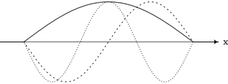
1.2 Probability amplitudes 5

Figure 1.1The two-slit interference experiment.

1.2 Probability amplitudes

Many branches of the social, physical and medical sciences make extensive use of probabilities, but quantum mechanics stands alone in theway that it calculates probabilities, for it always evaluates a probability pas the mod- square of a certain complex numberA:

p=|A|². (1.10)

The complex numberAis called theprobability amplitudeforp.

Quantum mechanics is the only branch of knowledge in which proba- bility amplitudes appear, and nobody understands why they arise. They give rise to phenomena that have no analogues in classical physics through the following fundamental principle. Suppose something can happen by two (mutually exclusive) routes,S orT, and let the probability amplitude for it to happen by routeSbeA(S) and the probability amplitude for it to happen by routeT beA(T). Then the probability amplitude for it to happen by one route or the other is

A(S orT) =A(S) +A(T). (1.11) This rule takes the place of the sum rule for probabilities, equation (1.3).

However, it is incompatible with equation (1.3), because it implies that the probability that the event happens regardless of route is

p(S orT) =|A(S or T)|²=|A(S) +A(T)|²

=|A(S)|²+A(S)A^∗(T) +A^∗(S)A(T) +|A(T)|²

=p(S) +p(T) + 2ℜ^e(A(S)A^∗(T)).

(1.12) That is, the probability that an event will happen is not merely the sum of the probabilities that it will happen by each of the two possible routes:

there is an additional term 2ℜ^e(A(S)A^∗(T)). This term has no counterpart in standard probability theory, and violates the fundamental rule (1.3) of probability theory. It depends on the phases of the probability amplitudes for the individual routes, which do not contribute to the probabilitiesp(S) =

|A(S)|² of the routes.

Whenever the probability of an event differs from the sum of the prob- abilities associated with the various mutually exclusive routes by which it can happen, we say we have a manifestation of quantum interference.

The term 2ℜ^e(A(S)A^∗(T)) in equation (1.12) is what generates quantum interference mathematically. We shall see that in certain circumstances the violations of equation (1.3) that are caused by quantum interference are not detectable, so standard probability theory appears to be valid.

How do we know that the principle (1.11), which has these extraordinary consequences, is true? The soundest answer is that it is a fundamental postulate of quantum mechanics, and that every time you look at a digital watch, or touch a computer keyboard, or listen to a CD player, or interact with any other electronic device that has been engineered with the help of quantum mechanics, you are testing and vindicating this theory. Our civilisation now quite simply depends on the validity of equation (1.11).

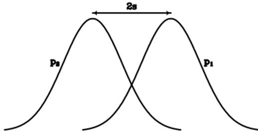
Figure 1.2 The probability distribu- tions of passing through each of the two closely spaced slits overlap.

1.2.1 Two-slit interference

An imaginary experiment will clarify the physical implications of the prin- ciple and suggest how it might be tested experimentally. The apparatus consists of an electron gun, G, a screen with two narrow slits S1 and S2, and a photographic plate P, which darkens when hit by an electron (see Figure 1.1).

When an electron is emitted by G, it has an amplitude to pass through slit S1 and then hit the screen at the pointx. This amplitude will clearly depend on the pointx, so we label itA1(x). Similarly, there is an amplitude A2(x) that the electron passed through S2 before reaching the screen atx.

Hence the probability that the electron arrives atxis

P(x) =|A1(x) +A2(x)|²=|A1(x)|²+|A2(x)|²+ 2ℜ^e(A1(x)A^∗₂(x)). (1.13)

|A1(x)|² is simply the probability that the electron reaches the plate after passing through S1. We expect this to be a roughly Gaussian distribution p1(x) that is centred on the value x1 of xat which a straight line from G through the middle of S1hits the plate. |A2(x)|²should similarly be a roughly Gaussian functionp2(x) centred on the intersection atx2 of the screen and the straight line from G through the middle of S2. It is convenient to write Ai =|Ai|e^iφi =√pie^iφi, whereφi is the phase of the complex number Ai. Then equation (1.13) can be written

p(x) =p1(x) +p2(x) +I(x), (1.14a) where theinterference termI is

I(x) = 2p

p1(x)p2(x) cos(φ1(x)−φ2(x)). (1.14b) Consider the behaviour of I(x) near the point that is equidistant from the slits. Then (see Figure 1.2)p1≃p2and the interference term is comparable in magnitude to p1 +p2, and, by equations (1.14), the probability of an electron arriving atxwill oscillate between ∼2p1 and 0 depending on the value of the phase differenceφ1(x)−φ2(x). In§2.3.4 we shall show that the phasesφi(x) are approximately linear functions ofx, so after many electrons have been fired from G to P in succession, the blackening of P atx, which will be roughly proportional to the number of electrons that have arrived at x, will show a sinusoidal pattern.

Let’s replace the electrons by machine-gun bullets. Then everyday ex- perience tells us that classical physics applies, and it predicts that the prob- ability p(x) of a bullet arriving at x is just the sum p1(x) +p2(x) of the probabilities of a bullet coming through S1 or S2. Hence classical physics does not predict a sinusoidal pattern inp(x). How do we reconcile the very different predictions of classical and quantum mechanics? Firearms manufac- turers have for centuries used classical mechanics with deadly success, so is the resolution that bullets do not obey quantum mechanics? We believe they do, and the probability distribution for the arrival of bulletsshould show a sinusoidal pattern. However, in§2.3.4 we shall find that quantum mechanics predicts that the distance ∆ between the peaks and troughs of this pattern

1.3 Quantum states 7 becomes smaller and smaller as we increase the mass of the particles we are firing through the slits, and by the time the particles are as massive as a bullet, ∆ is fantastically small ∼ 10⁻²⁹m. Consequently, it is not exper- imentally feasible to test whether p(x) becomes small at regular intervals.

Any feasible experiment will probe the value of p(x) averaged over many peaks and troughs of the sinusoidal pattern. This averaged value of p(x) agrees with the probability distribution we derive from classical mechanics because the average value ofI(x) in equation (1.14) vanishes.

1.2.2 Matter waves?

The sinusoidal pattern of blackening on P that quantum mechanics predicts proves to be identical to the interference pattern that is observed in Young’s double-slit experiment. This experiment established that light is a wave phe- nomenon because the wave theory could readily explain the existence of the interference pattern. It is natural to infer from the existence of the sinusoidal pattern in the quantum-mechanical case, that particles are manifestations of waves in some medium. There is much truth in this inference, and at an advanced level this idea is embodied in quantum field theory. However, in the present context of non-relativistic quantum mechanics, the concept of matter waves is unhelpful. Particles are particles, not waves, and they pass through one slit or the other. The sinusoidal pattern arises because proba- bility amplitudes are complex numbers, which add in the same way as wave amplitudes. Moreover, the energy density (intensity) associated with a wave is proportional to the mod square of the wave amplitude, just as the proba- bility density of finding a particle is proportional to the mod square of the probability amplitude. Hence, on a mathematical level, there is a one-to-one correspondence between what happens when particles are fired towards a pair of slits and when light diffracts through similar slits. But we cannot consistently infer from this correspondence that particles are manifestations of waves because quantum interference occurs in quantum systems that are much more complex than a single particle, and indeed in contexts where motion through space plays no role. In such contexts we cannot ascribe the interference phenomenon to interference between real physical waves, so it is inconsistent to take this step in the case of single-particle mechanics.

1.3 Quantum states

1.3.1 Quantum amplitudes and measurements

Physics is about the quantitative description of natural phenomena. A quan- titative description of a system inevitably starts by defining ways in which it can be measured. If the system is a single particle, quantities that we can measure are itsx,y and z coordinates with respect to some choice of axes, and the components of its momentum parallel to these axes. We can also measure its energy, and its angular momentum. The more complex a system is, the more ways there will be in which we can measure it.

Associated with every measurement, there will be a set of possible nu- merical values for the measurement – the spectrum of the measurement.

For example, the spectrum of the xcoordinate of a particle in empty space is the interval (−∞,∞), while the spectrum of its kinetic energy is (0,∞).

We shall encounter cases in which the spectrum of a measurement con- sists of discrete values. For example, in Chapter 7 we shall show that the angular momentum of a particle parallel to any given axis has spec- trum (. . . ,(k −1)¯h, k¯h,(k + 1)¯h, . . .), where ¯h is Planck’s constant h = 6.63×10⁻³⁴J s divided by 2π, andkis either 0 or ¹₂. When the spectrum is a set of discrete numbers, we say that those numbers are theallowedvalues of the measurement.

With every value in the spectrum of a given measurement there will be a quantum amplitude that we will find this value if we make the relevant measurement. Quantum mechanics is the science of how to calculate such amplitudes given the results of a sufficient number of prior measurements.

Imagine that you’re investigating some physical system: some particles in an ion trap, a drop of liquid helium, the electromagnetic field in a resonant cavity. What do you know about the state of this system? You have two types of knowledge: (1) a specification of the physical nature of the system (e.g., size & shape of the resonant cavity), and (2) information about the current dynamical state of the system. In quantum mechanics information of type (1) is used to define an object called the HamiltonianH of the system that is defined by equation (2.5) below. Information of type (2) is more subtle.

It must consist of predictions for the outcomes of measurements you could make on the system. Since these outcomes are inherently uncertain, your information must relate to the probabilities of different outcomes, and in the simplest case consists of values for the relevant probability amplitudes. For example, your knowledge might consist of amplitudes for the various possible outcomes of a measurement of energy, or of a measurement of momentum.

In quantum mechanics, then, knowledge about the current dynamical state of a system is embodied in a set of quantum amplitudes. In classical physics, by contrast, we can state with certainty which value we will measure, and we characterise the system’s current dynamical state by simply giving this value. Such values are often called ‘coordinates’ of the system. Thus in quantum mechanics a whole set of quantum amplitudes replaces a single number.

Complete sets of amplitudes Given the amplitudes for a certain set of events, it is often possible to calculate amplitudes for other events. The phe- nomenon of particle spin provides the neatest illustration of this statement.

Electrons, protons, neutrinos, quarks, and many other elementary par- ticles turn out to be tiny gyroscopes: they spin. The rate at which they spin and therefore the the magnitude of their spin angular momentum never changes; it is always p

3/4¯h. Particles with this amount of spin are called spin-half particlesfor reasons that will emerge shortly. Although the spin of a spin-half particle is fixed in magnitude, its direction can change. Conse- quently, the value of the spin angular momentum parallel to any given axis can take different values. In§7.4.2 we shall show that parallel to any given axis, the spin angular momentum of a spin-half particle can be either±¹2¯h.

Consequently, the spin parallel to thez axis is denotedsz¯h, where sz=±¹₂ is an observable with the spectrum{−¹₂,¹₂}.

In§7.4.2 we shall show that if we knowboth the amplitudea+ that sz

will be measured to be +¹₂ and the amplitudea₋ that a measurement will yield sz =−¹₂, then we can calculate from these two complex numbers the amplitudes b+ andb₋ for the two possible outcomes of the measurement of the spin alongany direction. If we know onlya+ (or onlya₋), then we can calculate neitherb+ norb₋ forany other direction.

Generalising from this example, we have the concept of a complete set of amplitudes: the set contains enough information to enable one to calculate amplitudes for the outcome of any measurement whatsoever.

Hence, such a set gives a complete specification of the physical state of the system. A complete set of amplitudes is generally understood to be a minimal set in the sense that none of the amplitudes can be calculated from the others.

The set{a₋, a+}constitutes a complete set of amplitudes for the spin of an electron.

1.3.2 Dirac notation

Dirac introduced the symbol|ψi, pronounced ‘ket psi’, to denote a complete

1.3 Quantum states 9 set of amplitudes for the system. If the system consists of a particle¹ trapped in a potential well, |ψi could consist of the amplitudesan that the energy is En, where (E1, E2, . . .) is the spectrum of possible energies, or it might consist of the amplitudes ψ(x) that the particle is found at x, or it might consist of the amplitudes a(p) that the momentum is measured to be p.

Using the abstract symbol|ψienables us to think about the system without committing ourselves to what complete set of amplitudes we are going to use, in the same way that the position vectorx enables us to think about a geometrical point independently of the coordinates (x, y, z), (r, θ, φ) or whatever by which we locate it. That is,|ψiis a container for a complete set of amplitudes in the same way that a vectorxis a container for a complete set of coordinates.

The ket|ψiencapsulates the crucial concept of aquantum state, which is independent of the particular set of amplitudes that we choose to quantify it, and is fundamental to several branches of physics.

We saw in the last section that amplitudes must sometimes be added: if an outcome can be achieved by two different routes and we do not monitor the route by which it is achieved, we add the amplitudes associated with each route to get the overall amplitude for the outcome. In view of this additivity, we write

|ψ3i=|ψ1i+|ψ2i (1.15) to mean that every amplitude in the complete set |ψ3i is the sum of the corresponding amplitudes in the complete sets |ψ1i and |ψ2i. This rule is exactly analogous to the rule for adding vectors becauseb3=b1+b2implies that each component ofb3 is the sum of the corresponding components of b1andb2.

Since amplitudes are complex numbers, for any complex number αwe can define

|ψ^′i=α|ψi (1.16)

to mean that every amplitude in the set |ψ^′i is αtimes the corresponding amplitude in|ψi. Again there is an obvious parallel in the case of vectors:

3bis the vector that hasxcomponent 3bx, etc.

1.3.3 Vector spaces and their adjoints

The analogy between kets and vectors proves extremely fruitful and is worth developing. For a mathematician, objects, like kets, that you can add and multiply by arbitrary complex numbers inhabit a vector space. Since we live in a (three-dimensional) vector space, we have a strong intuitive feel for the structures that arise in general vector spaces, and this intuition helps us to understand problems that arise with kets. Unfortunately our every- day experience does not prepare us for an important property of a general vector space, namely the existence of an associated ‘adjoint’ space, because the space adjoint to real three-dimensional space is indistinguishable from real space. In quantum mechanics and in relativity the two spaces are dis- tinguishable. We now take a moment to develop the mathematical theory of general vector spaces in the context of kets in order to explain the re- lationship between a general vector space and its adjoint space. When we are merely using kets as examples of vectors, we shall call them “vectors”.

Appendix D explains how these ideas are relevant to relativity.

For any vector spaceV it is natural to choose a set ofbasis vectors, that is, a set of vectors |ii that is large enough for it to be possible to

1Most elementary particles have intrinsic angular momentum or ‘spin’ (§7.4). A com- plete set of amplitudes for a particle such as electron or proton that has spin, includes information about the orientation of the spin. In the interests of simplicity, in our discus- sions particles are assumed to have no spin unless the contrary is explicitly stated, even though spinless particles are rather rare.

express any given vector|ψi as a linear combination of the set’s members.

Specifically, for any ket|ψithere are complex numbersai such that

|ψi=X

i

ai|ii. (1.17)

The set should be minimal in the sense that none of its members can be expressed as a linear combination of the remaining ones. In the case of ordi- nary three-dimensional space, basis vectors are provided by the unit vectors i,jandkalong the three coordinate axes, and any vectorbcan be expressed as the sumb=a1i+a2j+a3k, which is the analogue of equation (1.17).

In quantum mechanics an important role is played by complex-valued linear functions on the vector space V because these functions extract the amplitude for something to happen given that the system is in the state|ψi. Let hf| (pronounced ‘bra f’) be such a function. We denote by hf|ψi the result of evaluating this function on the ket|ψi. Hence, hf|ψiis a complex number (a probability amplitude) that in the ordinary notation of functions would be writtenf(|ψi). The linearity of the functionhf| implies that for any complex numbersα, β and kets|ψi,|φi, it is true that

hf| α|ψi+β|φi

=αhf|ψi+βhf|φi. (1.18) Notice that the right side of this equation is a sum of two products of complex numbers, so it is well defined.

To define a function on V we have only to give a rule that enables us to evaluate the function on any vector in V. Hence we can define the sum hh| ≡ hf|+hg|of two brashf|andhg|by the rule

hh|ψi=hf|ψi+hg|ψi (1.19) Similarly, we define the bra hp| ≡ αhf| to be result of multiplying hf| by some complex numberαthrough the rule

hp|ψi=αhf|ψi. (1.20) Since we now know what it means to add these functions and multiply them by complex numbers, they form a vector spaceV^′, called theadjoint space ofV.

Thedimensionof a vector space is the number of vectors required to make up a basis for the space. We now show thatV andV^′ have the same dimension. Let² {|ii}fori= 1, N be a basis for V. Then a linear function hf| on V is fully defined once we have given theN numbers hf|ii. To see that this is true, we use (1.17) and the linearity ofhf|to calculatehf|ψifor an arbitrary vector|ψi=P

iai|ii: hf|ψi=

XN i=1

aihf|ii. (1.21)

This result implies that we can define N functions hj| (j = 1, N) through the equations

hj|ii=δij, (1.22)

whereδij is 1 ifi=jand zero otherwise, because these equations specify the value that each brahj|takes on every basis vector|iiand therefore through (1.21) the value thathj|takes on any vectorψ. Now consider the following linear combination of these bras:

hF| ≡ XN j=1

hf|jihj|. (1.23)

2Throughout this book the notation{xi}means ‘the set of objectsxi’.

1.3 Quantum states 11 It is trivial to check that for any i we have hF|ii = hf|ii, and from this it follows thathF|=hf|because we have already agreed that a bra is fully specified by the values it takes on the basis vectors. Since we have now shown thatany bra can be expressed as a linear combination of theNbras specified by (1.22), and the latter are manifestly linearly independent, it follows that the dimensionality ofV^′ isN, the dimensionality ofV.

In summary, we have established that everyN-dimensional vector space V comes with anN-dimensional spaceV^′of linear functions onV, called the adjoint space. Moreover, we have shown that once we have chosen a basis {|ii}forV, there is an associated basis {hi|}forV^′. Equation (1.22) shows that there is an intimate relation between the ket|iiand the brahi|: hi|ii= 1 whilehj|ii= 0 forj 6=i. We acknowledge this relationship by saying thathi| is theadjointof|ii. We extend this definition of an adjoint to an arbitrary ket|ψias follows: if

|ψi=X

i

ai|ii then hψ| ≡X

i

a^∗_ihi|. (1.24) With this choice, when we evaluate the functionhψ|on the ket |ψiwe find

hψ|ψi=X

i

a^∗_ihi|X

j

aj|ji

=X

i

|ai|²≥0. (1.25) Thus for any state the number hψ|ψi is real and non-negative, and it can vanish only if |ψi= 0 because every ai vanishes. We call this number the lengthof|ψi.

The components of an ordinary three-dimensional vector b = bxi+ byj+bzk are real. Consequently, we evaluate the length-square of b as simply (bxi+byj+bzk)·(bxi+byj+bzk) =b²_x+b²_y+b²_z. The vector on the extreme left of this expression is strictly speaking the adjoint ofbbut it is indistinguishable from it because we have not modified the components in any way. In the quantum mechanical case eq. 1.25, the components of the adjoint vector are complex conjugates of the components of the vector, so the difference between a vector and its adjoint is manifest.

If |φi = P

ibi|ii and |ψi = P

iai|ii are any two states, a calculation analogous to that in equation (1.25) shows that

hφ|ψi=X

i

b^∗_iai, (1.26)

where the bi are the amplitudes that define the state|φi. Similarly, we can show that hψ|φi=P

ia^∗_ibi, and from this it follows that hψ|φi= hφ|ψi∗

. (1.27)

We shall make frequent use of this equation.

Equation (1.26) shows that there is a close connection between extract- ing the complex numberhφ|ψifromhφ|and|ψiand the operation of taking the dot product between two vectorsbanda.

1.3.4 The energy representation

Suppose our system is a particle that is trapped in some potential well. Then the spectrum of allowed energies will be a set of discrete numbersE0,E1,. . . and a complete set of amplitudes are the amplitudes ai whose mod squares give the probabilitiespiof measuring the energy to beEi. Let{|ii}be a set of basis kets for the space V of the system’s quantum states. Then we use the set of amplitudes aito associate them with a ket|ψithrough

|ψi=X

i

ai|ii. (1.28)

This equation relates a complete set of amplitudes {ai} to a certain ket

|ψi. We discover the physical meaning of a particular basis ket, say|ki, by examining the values that the expansion coefficientsai take when we apply equation (1.28) in the case|ki=|ψi. We clearly then have that ai = 0 for i 6= k and ak = 1. Consequently, the quantum state |ki is that in which we are certain to measure the value Ek for the energy. We say that |ki is a state of well defined energy. It will help us remember this important identification if we relabel the basis kets, writing|Eiiinstead of just|ii, so that (1.28) becomes

|ψi=X

i

ai|Eii. (1.29)

Suppose we multiply this equation through by hEk|. Then by the lin- earity of this operation and the orthogonality relation (1.22) (which in our new notation readshEk|Eii=δik) we find

ak=hEk|ψi. (1.30)

This is an enormously important result because it tells us how to extract from an arbitrary quantum state|ψithe amplitude for finding that the energy is Ek.

Equation (1.25) yields

hψ|ψi=X

i

|ai|²=X

i

pi= 1, (1.31)

where the last equality follows because if we measure the energy, we must findsome value, so the probabilitiespi must sum to unity. Thus kets that describe real quantum states must have unit length: we call kets with unit lengthproperly normalised. During calculations we frequently encounter kets that are not properly normalised, and it is important to remember that the key rule (1.30) can be used to extract predictions only from properly normalised kets. Fortunately, any ket|φi=P

ibi|iiis readily normalised: it is straightforward to check that

|ψi ≡X

i

bi

phφ|φi|ii (1.32)

is properly normalised regardless of the values of thebi.

1.3.5 Orientation of a spin-half particle

Formulae for the components of the spin angular momentum of a spin-half particle that we shall derive in §7.4.2 provide a nice illustration of how the abstract machinery just introduced enables us to predict the results of ex- periments.

If you measure one component, saysz, of the spinsof an electron, you will obtain one of two results, eithersz= ¹₂ or sz=−¹2. Moreover the state

|+iin which a measurement ofsz is certain to yield ¹₂ and the state |−iin which the measurement is certain to yield −¹₂ form a complete set of states for the electron’s spin. That is,any state of spin can be expressed as a linear combination of|+iand|−i:

|ψi=a₋|−i+a+|+i. (1.33) Letnbe the unit vector in the direction with polar coordinates (θ, φ).

Then the state|+,niin which a measurement of the component of salong nis certain to return ¹₂ turns out to be (Problem 7.12)

|+,ni= sin(θ/2) e^iφ/2|−i+ cos(θ/2) e^−iφ/2|+i. (1.34a)

1.3 Quantum states 13 Similarly the state |−,ni in which a measurement of the component of s alongnis certain to return−¹2 is

|−,ni= cos(θ/2) e^iφ/2|−i −sin(θ/2) e^−iφ/2|+i. (1.34b) By equation (1.24) the adjoints of these kets are the bras

h+,n|= sin(θ/2) e^−iφ/2h−|+ cos(θ/2) e^iφ/2h+|

h−,n|= cos(θ/2) e^−iφ/2h−| −sin(θ/2) e^iφ/2h+|. (1.35) From these expressions it is easy to check that the kets|±,ni are properly normalised and orthogonal to one another.

Suppose we have just measuredsz and found the value to be ¹₂ and we want the amplitudeA₋(n) to find−¹2 when we measuren·s. Then the state of the system is|ψi=|+iand the required amplitude is

A₋(n) =h−,n|ψi=h−,n|+i=−sin(θ/2)e^iφ/2, (1.36) so the probability of this outcome is

P₋(n) =|A₋(n)|²= sin²(θ/2). (1.37) This vanishes when θ= 0 as it should since then n= (0,0,1) son·s=sz, and we are guaranteed to findsz=¹₂ rather than−¹₂. P₋(n) rises to¹₂ when θ=π/2 andnlies somewhere in the x, y plane. In particular, if sz = ¹₂, a measurement ofsxis equally likely to return either of the two possible values

±₂¹.

Puttingθ=π/2,φ= 0 into equations (1.34) we obtain expressions for the states in which the result of a measurement ofsx is certain

|+, xi= 1

√2(|−i+|+i) ; |−, xi= 1

√2(|−i − |+i). (1.38) Similarly, insertingθ=π/2,φ=π/2 we obtain the states in which the result of measuringsy is certain

|+, yi= e^iπ/4

√2 (|−i −i|+i) ; |−, yi=e^iπ/4

√2 (|−i+ i|+i). (1.39) Notice that |+, xi and |+, yi are both states in which the probability of measuring sz to be ¹₂ is ¹₂. What makes them physically distinct states is that the ratio of the amplitudes to measure ±¹₂ forsz is unity in one case and i in the other.

1.3.6 Polarisation of photons

A discussion of the possible polarisations of a beam of light displays an interesting connection between quantum amplitudes and classical physics.

At any instant in a polarised beam of light, the electric vectorE is in one particular direction perpendicular to the beam. In a plane-polarised beam, the direction of E stays the same, while in a circularly polarised beam it rotates. A sheet of Polaroid transmits the component ofEin one direction and blocks the perpendicular component. Consequently, in the transmitted beam |E| is smaller than in the incident beam by a factor cosθ, whereθ is the angle between the incident field and the direction in the Polaroid that transmits the field. Since the beam’s energy flux is proportional to |E|², a fraction cos²θ of the beam’s energy is transmitted by the Polaroid.

Individual photons either pass through the Polaroid intact or are ab- sorbed by it depending on which quantum state they are found to be in

when they are ‘measured’ by the Polaroid. Let|→ibe the state in which the photon will be transmitted and |↑ithat in which it will be blocked. Then the photons of the incoming plane-polarised beam are in the state

|ψi= cosθ|→i+ sinθ|↑i, (1.40) so each photon has an amplitude a_→ = cosθ for a measurement by the Polaroid to find it in the state |→i and be transmitted, and an amplitude a_↑ = sinθ to be found to be in the state|↑i and be blocked. The fraction of the beam’s photons that are transmitted is the probability get through P_→=|a_→|² = cos²θ. Consequently a fraction cos²θ of the incident energy is transmitted, in agreement with classical physics.

The states |→iand |↑i form a complete set of states for photons that move in the direction of the beam. An alternative complete set of states is the set{|+i,|−i}formed by the state|+iof a right-hand circularly polarised photon and the state|−iof a left-hand circularly polarised photon. In the laboratory a circularly polarised beam is often formed by passing a plane polarised beam through a birefringent material such as calcite that has its axes aligned at 45^◦ to the incoming plane of polarisation. The incoming beam is resolved into its components parallel to the calcite’s axes, and one component is shifted in phase byπ/2 with respect to the other. In terms of unit vectors ˆex and ˆey parallel to the calcite’s axes, the incoming field is

E= E

√2ℜ

(ˆex+ ˆey)e^−iωt (1.41) and the outgoing field of a left-hand polarised beam is

E₋= E

√2ℜ

(ˆex+ iˆey)e^−iωt , (1.42a) while the field of a right-hand polarised beam would be

E+= E

√2ℜ

(ˆex−iˆey)e^−iωt . (1.42b) The last two equations express the electric field of a circularly polarised beam as a linear combination of plane polarised beams that differ in phase.

Conversely, by adding (1.42b) to equation (1.42a), we can express the electric field of a beam polarised along thexaxis as a linear combination of the fields of two circularly-polarised beams.

Similarly, the quantum state of a circularly polarised photon is a linear superposition of linearly-polarised quantum states:

|±i= 1

√2(|→i ∓i|↑i), (1.43) and conversely, a state of linear polarisation is a linear superposition of states of circular polarisation:

|→i= 1

√2(|+i+|−i). (1.44) Whereas in classical physics complex numbers are just a convenient way of representing the real function cos(ωt+φ) for arbitrary phase φ, quantum amplitudes are inherently complex and the operatorℜis not used. Whereas in classical physics a beam may be linearly polarised in a particular direction, or circularly polarised in a given sense, in quantum mechanics an individual photon has an amplitude to be linearly polarised in a any chosen direction andan amplitude to be circularly polarised in a given sense. The amplitude to be linearly polarised may vanish in one particular direction, or it may vanish for one sense of circular polarisation. In the general case the photon will have a non-vanishing amplitude to be polarised in any direction and any sense. After it has been transmitted by an analyser such as Polaroid, it will certainly be in whatever state the analyser transmits.

Problems 15

1.4 Measurement

Equation (1.28) expresses the quantum state of a system|ψias a sum over states in which a particular measurement, such as energy, is certain to yield a specified value. The coefficients in this expansion yield as their mod-squares the probabilities with which the possible results of the measurement will be obtained. Hence so long as there is more than one term in the sum, the result of the measurement is in doubt. This uncertainty does not reflect shortcom- ings in the measuring apparatus, but is inherent in the physical situation – any defects in the measuring apparatus will increase the uncertainty above the irreducible minimum implied by the expansion coefficients, and in§6.3 the theory will be adapted to include such additional uncertainty.

Here we are dealing with ideal measurements, and such measurements are reproducible. Therefore, if a second measurement is made immediately after the first, the same result will be obtained. From this observation it follows that the quantum state of the system is changed by the first mea- surement from |ψi=P

iai|iito |ψi= |Ii, where |Ii is the state in which the measurement is guaranteed to yield the value that was obtained by the first measurement. The abrupt change in the quantum state from P

iai|ii to|Iithat accompanies a measurement is referred to as thecollapse of the wavefunction.

What happens when the “wavefunction collapses”? It is tempting to suppose that this event is not a physical one but merely an updating of our knowledge of the system: that the system was already in the state|Ii before the measurement, but we only became aware of this fact when the measurement was made. It turns out that this interpretation is untenable, and that wavefunction collapse is associated with a real physical disturbance of the system. This topic is explored further in§6.5.

Problems

1.1 What physical phenomenon requires us to work with probability am- plitudes rather than just with probabilities, as in other fields of endeavour?

1.2 What properties cause complete sets of amplitudes to constitute the elements of a vector space?

1.3 V^′ is the adjoint space of the vector space V. For a mathematician, what objects compriseV^′?

1.4 In quantum mechanics, what objects are the members of the vector spaceV? Give an example for the case of quantum mechanics of a member of the adjoint spaceV^′ and explain how members ofV^′ enable us to predict the outcomes of experiments.

1.5 Given that|ψi= e^iπ/5|ai+ e^iπ/4|bi, expresshψ|as a linear combination ofha|andhb|.

1.6 What properties characterise the braha|that is associated with the ket

|ai?

1.7 An electron can be in one of two potential wells that are so close that it can “tunnel” from one to the other (see§5.2 for a description of quantum- mechanical tunnelling). Its state vector can be written

|ψi=a|Ai+b|Bi, (1.45) where|Aiis the state of being in the first well and|Biis the state of being in the second well and all kets are correctly normalised. What is the probability of finding the particle in the first well given that: (a) a= i/2; (b) b = e^iπ; (c)b=¹₃ + i/√

2?

1.8 An electron can “tunnel” between potential wells that form a chain, so its state vector can be written

|ψi= X∞

−∞

an|ni, (1.46a)

where|niis the state of being in then^th well, wherenincreases from left to right. Let

an= 1

√2 −i

3 |n|/2

e^inπ. (1.46b)

a. What is the probability of finding the electron in then^th well?

b. What is the probability of finding the electron in well 0 or anywhere to the right of it?

2

Operators, measurement and time evolution

In the last chapter we saw that each quantum state of a system is represented by a point or ‘ket’ |ψi that lies in an abstract vector space. We saw that states for which there is no uncertainty in the value that will be measured for a quantity such as energy, form a set of basis states for this space – these basis states are analogous to the unit vectors i, j and k of ordinary vector geometry. In this chapter we develop these ideas further by showing how every measurable quantity such as position, momentum or energy is associated with an operator on state space. We shall see that the energy operator plays a special role in that it determines how a system’s ket |ψi moves through state space over time. Using these operators we are able at the end of the chapter to study the dynamics of a free particle, and to understand how the uncertainties in the position and momentum of a particle are intimately connected with one another, and how they evolve in time.

2.1 Operators

A linear operator on the vector space V is an object Q that transforms kets into kets in a linear way. That is, if |ψi is a ket, then |φi = Q|ψi is another ket, and if|χiis a third ket andαandβ are complex numbers, we have

Q α|ψi+β|χi

=α(Q|ψi) +β(Q|χi). (2.1) Consider now the linear operator

I=X

i

|iihi|, (2.2)

where {|ii} is any set of basis kets. I really is an operator because if we apply it to any ket|ψi, we get a linear combination of kets, which must itself be a ket:

I|ψi=X

i

|iihi|ψi=X

i

(hi|ψi)|ii, (2.3)