On the ambiguity of the reaction rate constants in multivariate curve resolution for reversible first-order reaction systems.
Henning Schr¨odera, Mathias Sawalla, Christoph Kubisb, Detlef Selentb, Dieter Hessc, Robert Frankec,d, Armin B¨ornerb, Klaus Neymeyra,b
aUniversit¨at Rostock, Institut f¨ur Mathematik, Ulmenstrasse 69, 18057 Rostock, Germany
bLeibniz-Institut f¨ur Katalyse, Albert-Einstein-Strasse 29a, 18059 Rostock, Germany
cEvonik Performance Materials GmbH, Paul-Baumann Strasse 1, 45772 Marl, Germany
dLehrstuhl f¨ur Theoretische Chemie, Ruhr-Universit¨at Bochum, 44780 Bochum, Germany
Abstract
If for a chemical reaction with a known reaction mechanism the concentration profiles are accessible only for certain species, e.g. only for the main product, then often the reaction rate constants cannot uniquely be determined from the concentration data. This is a well-known fact which includes the so-called slow-fast ambiguity.
This work combines the question of unique or non-unique reaction rate constants with factor analytic methods of chemometrics. The idea is to reduce the rotational ambiguity of pure component factorizations by considering only those concentration factors which are possible solutions of the kinetic equations for a properly adapted set of reaction rate constants. The resulting set of reaction rate constants corresponds to those solutions of the rate equations which appear as feasible factors in a pure component factorization.
The new analysis of the ambiguity of reaction rate constants extends recent research activities on the Area of Feasible Solutions (AFS). The consistency with a given chemical reaction scheme is shown to be a valuable tool in order to reduce the AFS. The new methods are applied to model and experimental data.
Key words: spectral recovery, factor analysis, nonnegative matrix factorization, kinetic modeling, feasible rate constants, area of feasible solutions.
1. Introduction
Multivariate curve resolution techniques are well- established and powerful tools to extract pure compo- nent information from spectroscopic data. Unfortu- nately, these methods suffer from the non-uniqueness of the possible nonnegative factorizations. Usually a con- tinuum of factorizations exists. This fact is well-known under the keyword of rotational ambiguity [1, 2]. If ad- ditionally soft- and/or hard-constraints are imposed on the solutions, then one can determine a unique solution.
In general, the non-uniqueness of the nonnegative fac- torizations can be represented by drawing the sets of all possible concentration profiles or all possible spectra in the form of feasible bands [3]. Alternatively, the area of feasible solutions (AFS) [4, 5, 6, 7, 8, 9] is a low- dimensional representation of the set of all nonnegative concentration profiles and all nonnegative pure compo- nent spectra which appear in possible factorizations of the spectral data matrix. In this sense, we consider the AFS methodology as a global approach since it pro-
vides an overview of the full range of all nonnegative factorizations. In recent works [10, 11, 12] various soft constraints have directly been applied to the AFS in or- der to reduce the rotational ambiguity. This reduction of the ambiguity is reflected by drastically smaller subsets of the original AFS. These subsets represent the possi- ble factorizations which additionally meet the soft con- straints.
In this work the global approach including the subse- quent reduction step is extended to kinetic hard-models.
A kinetic hard-model is well-known to be a very power- ful restriction for a multivariate curve resolution method [13, 14, 1, 15]. The parameters of such kinetic models, namely the reaction rate constants, have not to be known in advance, but can be computed during the model- fitting process by means of an optimization procedure.
It is a well-known fact [16, 14, 17, 18] that sometimes the reaction rate constants cannot uniquely be deter- mined from incomplete concentration data, e.g. if the concentration values are only accessible for the main
product of the reaction. This is a possible situation if, e.g., an isolated spectral peak of the main product can be used to extract the concentration information, see [15]. For first-order consecutive chemical reactions the non-uniqueness is also known as the “slow-fast ambi- guity”. In case of the slow-fast ambiguity for instance, the concentration profile of the main reaction product depends in a symmetric way on two of the reaction rate constants. In other words, these two rate constants can be permuted without changing the time-dependent con- centration function of this chemical component. Pos- sibly but not necessarily this change can be associated with negative entries in the spectral factor; this issue is also discussed in this paper. A general analysis of these questions is given in [19, 20], where identifiability and distinguishability for first-order and more general sys- tems are the key concepts. Identifiability means that ki- netic parameters for an assumed kinetic can be found in a unique way and distinguishability implies that one can determine a unique reaction scheme.
The aim of this paper is to combine the question of unique or non-unique reaction rate constants with model-free curve resolution methods for the case of general first-order kinetics. The rotational ambiguity inherent to these pure component factorizations is re- duced by considering only those concentration factors which are possible solutions of the kinetic equations for properly adapted reaction rate constants. To this end we introduce the setK of rate constants whose associated solutions of the kinetic equations result in feasible con- centration factors. Further, the subsetK+ ofK is de- fined by taking only those reaction rate constants whose associated concentration factors C can be supplemented by nonnegative spectral factors A so that the product CA reconstructs the initial spectral observation matrix. Fi- nally, the set K+ is extended to a set of feasible rate constants with respect to perturbationsKε+by introduc- ing an accepted noise levelε ≥ 0. A central result of this paper is a theorem which characterizes the setKby a similarity condition for the Kirchhoffmatrix.
1.1. Organization of the paper
The paper is organized as follows: Section 2 reca- pitulates an elementary model example of the slow-fast ambiguity for a first-order consecutive reaction system with three components [16, 17]. Section 3 shows how a kinetic hard-model can be implemented by a cost func- tion which depends only on the reaction rate constants.
The central definitions of the sets of consistent and fea- sible reaction rate constants are introduced in Section 4.
Additionally this section contains the central results of
the paper, namely Theorem 4.3 on a simple characteri- zation of consistent vectors of rate constants. Section 5 is devoted to an extension of the set of feasible reaction rate constants to noisy data. Finally, in Section 6 the new concepts are applied to various first-order reaction schemes. The associated sets of consistent and feasible reaction rate constants are mathematically derived and numerically computed.
2. Rate constants ambiguity for an elementary first- order consecutive reaction
The kinetic equation of a first-order chemical reaction with given initial concentrations c0has the form of the vectorial initial value problem
dc(t)
dt =M(k) c(t), c(t1)=c0. (2.1) Therein the s×s matrix M(k) is the kinetic or Kirchhoff matrix and s is the number of chemical components. It depends on nonnegative reaction rate constants, which are written by a vector k∈Rqwith q components.
A simple consecutive first-order reaction scheme with three components is sufficient in order to demon- strate a certain non-uniqueness of the reaction rate con- stants, which is known as the slow-fast ambiguity [16].
Example 2.1. We consider the first order consecutive reaction
X−→k1 Y −→k2 Z
with the initial concentrations (1,0,0) for X, Y and Z.
The associated kinetic matrix or Kirchhoffmatrix reads
M(k)=
−k1 0 0 k1 −k2 0
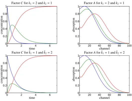
0 k2 0
. (2.2) The solution of the initial value problem (2.1) for these initial concentrations and this Kirchhoff matrix with (k1,k2) = (2,1) results in concentration profiles which are shown in the first row of Figure 1. Additionally, this first row in Figure 1 shows the three pure compo- nent spectra which we have assumed. The associated series of mixture spectra, i.e. the rows of the matrix D, are plotted in Figure 2. A second set of rate constants, namely (˜k1,˜k2)=(1,2), exists, which is consistent with the spectral data matrix D. The resulting concentration profiles and pure component spectra are shown in the second row of Figure 1.
This example problem allows to explain the slow-fast 2
0 2 4 6 0
0.2 0.4 0.6 0.8 1
time
concentration
Factor C for k1=2 and k2=1
0 20 40 60 80 100
0 0.2 0.4 0.6 0.8 1
channel
absorption
Factor A for k1=2 and k2=1
0 2 4 6
0 0.2 0.4 0.6 0.8 1
time
concentration
Factor C for ˜k1=1 and ˜k2=2
0 20 40 60 80 100
0 0.2 0.4 0.6 0.8 1
channel
absorption
Factor A for ˜k1=1 and ˜k2=2
Figure 1: Two different factorizations for the consecutive reaction described in Example 2.1. The associated series of spectra for the mixture is shown in Figure 2. The two concentration factors are consistent with the kinetic model X−−→k1 Y−−→k2 Z for different sets of kinetic rate constants.
The factor A is nonnegative for each of these factorizations. Thus the two factorizations are feasible and consistent with the given kinetic model.
ambiguity [21, 16, 17]. The crucial point is that the two concentration profiles of the reaction product Z (in red color) in the left column in Figure 1 are identical even though the vectors of rate constants are different. In other words, if the concentration of Z is an observable quantity, then at least two sets of rate constants exist, which result in the same concentration profile.
3. Kinetic hard-modeling and pure component fac- torizations
We consider the following pure component factoriza- tion problem: For a given spectral data matrix D∈Rm×n a factorization D=CA is wanted with nonnegative fac- tors C ∈ Rm×sand A∈ Rs×n. The spectral data matrix D contains in its m rows the mixture spectra taken at m times from a chemical reaction system. Each spec- tral profile contains absorption values at n frequencies.
The number s represents the assumed active and inde- pendent chemical components. We understand an in- dependent chemical component as a chemical compo- nent which increases the rank of the spectral data ma- trix D by 1. Thus s is the rank of the matrices D,C and A for noise-free and non-perturbed data. The matrices
C and A contain the concentration profiles and spectra of the s pure components. For an introduction to this factorization problem see, e.g., [1] and the references therein. Usually, the nonnegative factorization D=CA is not unique. Instead, continua of nonnegative matrices C and A exist. These sets of feasible solutions can be represented by the low-dimensional AFS plots.
We are interested in a chemically correct and inter- pretable factorization for which the s columns of the concentration factor C describe the concentration pro- files of the s chemical components along the time axis.
The associated factor A contains in its rows the pure component spectra. The a priori knowledge of a chem- ical reaction scheme is a very useful information in order to determine chemically relevant factorizations D = CA. In the best possible case only a single so- lution is consistent with the chemical reaction scheme.
A by-product of such model-fit computations are opti- mally adapted reaction rate constants. In other cases, not only a single solution can be identified, but a small subset of the initial set of all nonnegative factorizations of D. With respect to the AFS representation of these solutions, such a subset can have the form of a one- dimensional curve within a two-dimensional AFS set 3
0 20 40 60 80 100 0
0.2 0.4 0.6 0.8 1
Figure 2: Series of mixture spectra for the three-component consecutive reaction X→Y→Z, see Example 2.1.
(for the case of a three-component system).
3.1. A cost function on nonnegativity and consistency with a kinetic hard-model
A certain chemical reaction scheme can be integrated into a pure component factorization D=CA. This of- ten allows to reduce the rotational ambiguity drastically.
This integration can be done in the form of a hard con- straint by considering a proper cost functional within an SVD-based optimization procedure [1, 13, 22, 23]. Al- ternatively, the hard model approach can be combined with additional soft constraints in a joint optimization, see e.g. [15].
In the following, we use the hard model approach.
This means that we construct a cost function f (k) which depends only on the (unknown) vector k ∈ Rq of re- action rate constants. By solving the associated initial value problem (IVP), solely those concentration pro- files are considered as possible factors C=C(ode)(k)m+×s which fulfill the IVP (2.1) and for which an associated nonnegative spectral factor A exists so that CA approxi- mates the given mixture data matrix D. Optimal values of the rate constants are computed by a numerical min- imization of the cost function. We still have to explain how the time-continuous solution of the IVP
c(t)=
c1(t) ... cs(t)
∈Rs (3.1) is related to the matrix factor C(ode)(k) ∈ Rm+×s. This matrix results from an evaluation of the concentration functions along the time grid t1 <t2 <· · ·<tm. Thus C(ode)(k) is completely determined by the vector of rate constants k. Finally, D≈UΣVT is a truncated singular value decomposition [24] with the rank s, which is the
number of independent species. The numerical evalua- tion of the cost function for a given vector k is summa- rized in the steps:
1. C(ode)(k) is computed by solving the initial value problem (2.1).
2. The s×s matrix T =(C(ode)(k))+UΣis computed with the pseudo-inverse (C(ode)(k))+ of C(ode)(k).
(By the left-multiplication with the pseudo-inverse a least-squares problem is solved with respect to the s-dimensional column space of U.)
3. The matrix factors C=UΣT−1and A=T VT are calculated.
4. The value of the cost function f (k) is f (k)=
Xm
i=1
Xs
j=1
min Ci j
maxl(Cl j),0!2
+
Xs
i=1
Xn
j=1
min Ai j
maxl(Ail),0!2
+kC(ode)(k)−Ck2F.
(3.2)
Therein the squared Frobenius normk · k2F is the sum of squares of its argument.
This approach is closely related to the pure hard- modeling of de Juan et al. in [13]. A minor difference is that we expand the time-discrete concentration with respect to the left singular values of D, which means no difference for model data and amounts to a low-rank ap- proximation for perturbed data. In contrast to the well- known hard-soft MCR methods, the matrices C and A are completely determined by the s×s matrix T , which again is directly related to the matrix C(ode)(k), see steps 2 and 3 of the cost function. This underlines the high impact of the kinetic model on the pure component fac- tors C and A.
4
For model data, which have been generated from a given kinetic model, no low-rank approximation is nec- essary as the data matrix has at most the rank s (aside from rounding errors). Then minkf (k) = 0 holds and the associated matrix C(ode)(k) coincides with the matrix C.
In general cases, additional vectors of rate constants
˜k can exist, which also fulfill f (˜k) =0. In such cases, the kinetic model does not provide sufficient informa- tion in order to restrict the rotational ambiguity only to a single pure component factorization D = CA. Such ambiguities are well known for irreversible consecutive chemical reactions; cf. Example 2.1.
4. Parameter ambiguity for general first-order ki- netics
The ambiguity of the reaction rate constants for gen- eral first-order reaction systems is analyzed in this sec- tion. The central result of this section is Theorem 4.3 which provides a simple criterion for determining sets of rate constants that are consistent with the factoriza- tion of the given spectral data.
4.1. Definitions of sets of consistent and feasible reac- tion rate constants
We assume that the given spectral data matrix D ∈ Rm×n has at least one factorization D = CA with non- negative factors C ∈ Rm×sand A∈ Rs×n. Therein, the s columns of the concentration factor C should be in- terpreted as the concentration profiles of the s chemical components along the time axis. The m entries of each column of C are the concentration values for the points in time t1, . . . ,tm. Finally, we assume that the concentra- tion factor C is consistent with a vector k∈ Rqof non- negative reaction rate constants in the following sense:
The initial value problem (2.1) with the Kirchhoffma- trix M(k) has a solution c(t)=(c1(t), . . . ,cs(t))T ∈Rsso that the evaluation of these s concentration profiles for the points in time t1, . . . ,tmreproduces the matrix factor C. Mathematically this evaluation with respect to the grid points t1, . . . ,tmreads
C=
c1(t1) . . . cs(t1)
... ...
c1(tm) . . . cs(tm)
=:Tc(t). (4.1) The last equation defines the time grid discretization op- eratorT which evaluates the time-continuous solution c(t) of (2.1) on the given time grid. This results in the matrix C.
With these preparations we define the set of D- consistent rate constants as follows:
Definition 4.1 (Set of D-consistent reaction rate con- stants). Let D = UΣVT be the singular value decom- position of the rank-s matrix D ∈ Rm×n. The set of D- consistent reaction rate constants k∈Rqis defined as
K ={k∈Rq: c(t) solves (2.1), C=Tc(t) and
∃T ∈Rs×s,rank(T )=s and C=UΣT−1}. (4.2) In words the setK of D-consistent rate constants com- prises all reaction rate constants whose associated solu- tion c(t) of (2.1) on the discrete time grid t1, . . . ,tmcan be represented by the left singular vectors of D, i.e. the columns of U. (Sometimes we call the D-consistency simply consistency.)
This definition of the D-consistent rate constant is not sufficient to guarantee that the concentration factor C can be supplemented by a nonnegative spectral factor A in a way that the reconstruction D=CA holds. This ad- ditional requirement is part of the following definition.
Definition 4.2 (Set of nonnegatively feasible rate con- stants).
K+={k∈Rq: c(t) solves (2.1), C=Tc(t) and
∃T ∈Rs×s, rank(T )=s, C=UΣT−1 with A=T VT ≥0}.
(4.3) The definition of the setK+, in comparison to (4.2), contains the additional demand that A ≥ 0. Conse- quently it holds that K+ ⊆ K. For the consecutive reaction from Example 2.1 the set of D-consistent re- action rate constants is equal to the set of nonnegatively feasible rate constants. This means that K = K+ = {(2,1),(1,2)}.
4.2. Analysis by the eigenvalues of the Kirchhoffmatrix The set K of D-consistent rate constants can easily be characterized by the set of the eigenvalues of the ki- netic matrix M(k) in (2.1). Starting from a certain D- consistent rate constant vector k∗∈ K, a further vector k is also contained inKif M(k∗) and M(k) are similar ma- trices. (Similarity of M(k) and M(k∗) means that a reg- ular matrix Z ∈Rs×sexists so that M(k∗)=Z−1M(k)Z.) The following theorem contains the details.
Theorem 4.3. Let D ∈ Rm×n be a nonnegative matrix with rank(D)=s so that a matrix factorization D=CA with C ∈ Rm×s and A ∈ Rs×n exists. For this D the 5
vector k∗∈Rqis assumed to be a vector of D-consistent rate constants in the sense of Definition 4.1. This means that
Tc∗(t)=C∗=UΣ(T∗)−1 (4.4) with a regular s×s matrix T∗. Then the following equiv- alence holds:
The vector k ∈Rq+is D-consistent, if and only if the matrices M(k) and M(k∗) are similar matrices, i.e., they have the same sets of eigenvalues.
The proof of this theorem is postponed to Appendix A.
Remark 4.4. 1. Theorem 4.3 shows that the set membership of a certain k to the set K of D- consistent reaction rate constants, see Definition 4.1, can simply be decided by testing the similar- ity of the matrices M(k) and M(k∗) with k∗ ∈ K. Similar matrices, this is written as M(k)∼M(k∗), have the same eigenvalues and their equal eigen- values can be paired in a way that the associated eigenspaces have the same dimensions. (In the lan- guage of linear algebra, the sets of eigenvalues of M(k) and M(k∗) are the same and in the case of multiple eigenvalues any eigenvalue of M(k) is as- sociated with the same eigenvalue of M(k∗) and these eigenvalues have the same geometric multi- plicity, see [24].) With the similarity operator∼ this can compactly be written as
K=n
k∈Rq: M(k)∼M(k∗)o
. (4.5)
2. Numerically, Equation (4.5) can approximately be checked by the simple and computationally cheap computation of the sets of eigenvalues of M(k) and M(k∗). If M(k) and M(k∗) have equal eigenvalues (equality is meant with respect to a proper multiple of the machine precision) and if in the case of mul- tiple eigenvalues all geometric multiplicities are the same, then M(k)∼M(k∗) holds. Numerically, the non-diagonalizabilty of a matrix (such a ma- trix is often called defective) cannot be checked as the Jordan normal form of a matrix cannot be com- puted numerically. The key point is that a proper arbitrarily small perturbation of a defective ma- trix can transform this matrix into a diagonalizable matrix (with a large condition number).
3. Theorem 4.3 provides a simple criterion on D- consistency in the sense of Definition 4.1. This cri- terion does not guarantee the nonnegativity of the factor A. If additionally the existence of a non-
negative factor A is required, thenKreduces to its subsetK+of nonnegatively feasible rate constants.
4.3. Graphical presentation ofK andK+
If the first-order chemical reaction system is de- scribed by a number of q rate constants, then the setsK andK+are subsets of the q-dimensional space. How- ever only for q=2 and q=3 a graphical representation of these sets is easily possible by a 2D or 3D plot. Ev- ery opportunity should be taken in order to reduce the dimension of the graphical representation for the cases with q ≥4. A reduction from the dimension q to q−1 is possible in the following way:
1. Similar matrices have the same trace (sum of di- agonal elements or, equivalently, sum of eigenval- ues). Hence a constantψexists so that
ψ=−
Xq
i=1
λi=−trace(M(k)) (4.6) for all k∈ K. Theλiare the eigenvalues of M(k).
2. For a first-order chemical reaction system the neg- ative trace of the Kirchhoffmatrix M(k∗) with k∗∈ Kequals
Xq
i=1
ki=ψ
as the ith subreaction contributes the term−ki to the diagonal of the KirchhoffmatrixK; for an il- lustration of this relation see the example systems in Sections 6.2, 6.3 and 6.4.
3. A combination of the last two equations shows that the jth rate constant kj for j ∈ {1, . . . ,q}can be expressed as
kj=ψ−
Xq
i=1i,j
ki. (4.7)
Hence the linear relation (4.7) allows to present the sets K andK+within a (q−1)-dimensional space.
4.4. Numerical computation ofKandK+
The numerical computation of the set K of all vec- tors of D-consistent reaction rate constants, see Defi- nition 4.1, requires very long computation times. For each possible k an initial value problem is to be solved in order to determine the matrix C(ode)(k). The result of Theorem 4.3 is that initial value problems are not be solved any longer. Instead an eigenvalue problem is to be solved for the small s×s Kirchhoffmatrix M(k). This 6
is a simple and computationally very cheap step. Addi- tionally, Section 4.3 shows thatK can graphically be represented in a (q−1)-dimensional space. A straight- forward strategy for the computation ofK is a system- atic grid search. Therefore we cover a proper bounded subset of the Rq−1 by an equidistant grid. For each grid point, the grid points are vectors of rate constants, it is checked whether or not this point fulfills the D- consistency. A comparable grid search has been used in [25] for the computation of the area of feasible solu- tions.
The starting point for the grid search algorithm is a certain D-consistent rate constant k∗. Such an ini- tial solution can be calculated by using a proper hard- modeling kinetic procedure as used in [13, 1]. Then the grid search can be started. For very simple reaction sys- tems the whole computation can be done analytically, see Section 6 for an example. In the general case, a numerical approximation ofKis the only practical ap- proach.
Finally, the subsetK+of nonnegatively feasible rate constants can be extracted fromK by checking compu- tationally the nonnegativity of the factor A according to Definition 4.2.
4.5. Link to the area of feasible solutions
The area of feasible solutions (AFS), e.g. see [4, 5, 6, 7, 8, 9], represents the set of all factorizations D=CA with nonnegative factors C and A for a given spectral data matrix D. In more detail, the concentrational AFS which is denoted by MC in [7] is a low-dimensional representation of the set of all nonnegative factors C.
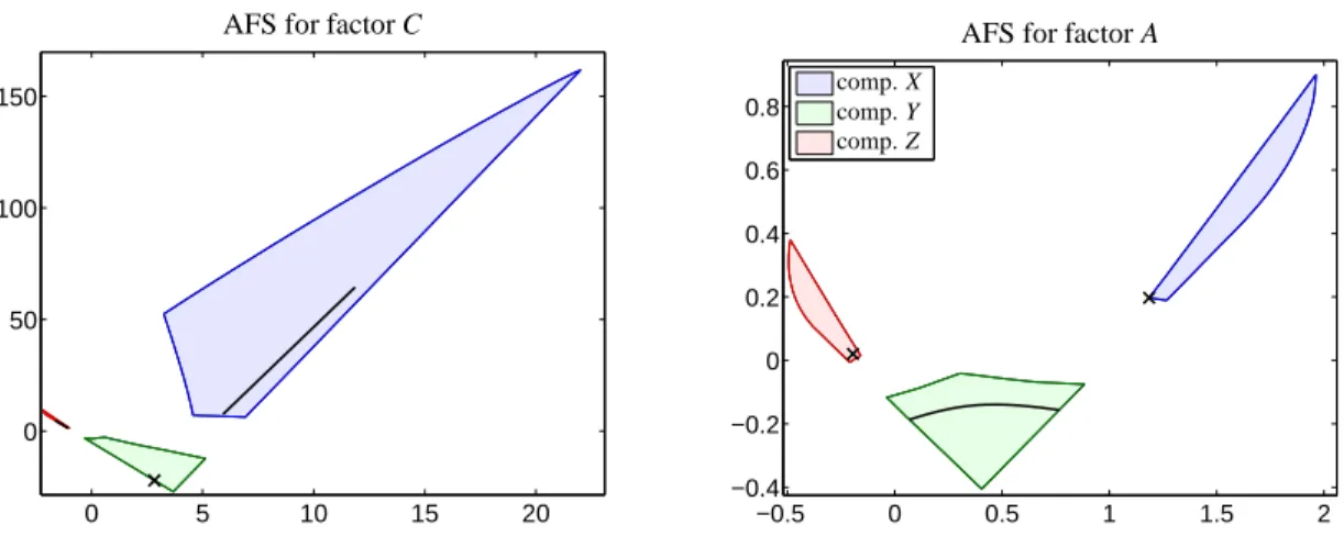
Analogously, the spectral AFSMAis a low-dimensional representation of all spectral factors A. The AFS is com- puted only by using the spectral data matrix D. The AFS does not include a consistency check of the non- negative solutions in C and A with a kinetic model of the reaction. This fact opens the possibility to combine the information on the set of nonnegatively feasible rate constantsK+with the AFS construction. The feasibility condition by Definition 4.2 imposes an additional con- straint on the areas of feasible solutionsMC andMA. Hence subsets of the AFS can be identified which repre- sent those factorizations of D that are additionally con- sistent with the underlying kinetic model. In Section 6.7 and Figure 14 numerical results of such a combination ofMCandMAwith a kinetic model are presented.
An interesting additional feature of the setK+is that the scaling information for the factors C and A is known as these factors result from the solution C(ode)of an ini- tial value problem. All this provides the selected AFS
solutions with an absolute scaling whenever a kinetic model of the reaction is accessible.
4.6. Application to data without sign restrictions Up to now we have always assumed that the matrix D contains only nonnegative absorption data. How- ever, Definition 4.1 of the set K describes the consis- tency with the kinetic model and does not require D to be a nonnegative matrix. At first, the analysis by the set K+ includes that the spectral factor A is a com- ponentwise nonnegative matrix. Hence, any spectro- scopic technique which underlies the bilinear Lambert- Beer law can be analyzed in the sense of the setK. We have tested this for simulated circular dichroism spec- troscopic data.
5. Computation ofK+for perturbed data
Section 4 contains an analysis of the ambiguity of the kinetic rate constants for first-order kinetics. Up to now this analysis is restricted to non-perturbed model data and cannot be applied to experimental data with a nonzero noise-to-signal ratio. For experimental data the minimum of the cost function f (k), see Equation (3.2), is usually larger than zero. Hence the definition of the set of D-consistent rate constants K in Equa- tion (4.2) cannot be applied in its strict sense, since the non-perturbed solution C(ode) of the initial value prob- lem cannot precisely be reconstructed from the left sin- gular vectors of D.
In order to overcome this problem and in order to an- alyze the sensitivity of the reaction rate constants, we define the set of feasible rate constantsKε+for a noise level whose magnitude is controlled by the parameter ε. The setKε+contains all rate constants for which the cost function f (k) from Equation (3.2) returns a value not larger thanε. The following algorithm for the com- putation ofKε+uses the setKas its starting point.
5.1. Definition of the set of feasible rate constants for perturbed data
The set of nonnegatively feasible rate constantsKε+
with respect to the noise levelε≥0 is defined to be Kε+={k∈Rq+: f (k)≤ε}. (5.1) Therein, the cost function f (k) is given in (3.2). By the construction of f the inequality f (k)≤εguarantees that negative entries of C and A are bounded from below and that C(ode)is re-constructable from the left singular vectors except for a minor error which tends to zero if 7
εtends to zero. For the limit caseε = 0 it holds that K0+=K+.
For perturbed data the trace invariance property from Section 4.3 is no longer true. In other wordsPq
i=1λi is not constant in cases withε >0. Hence the representa- tion ofK+for a system with q rate constants can only be given in theRq+and not in theRq+−1.
5.2. Algorithmic approach for the computation ofKε+
In Section 4 a strategy has been developed for the computation of K and K+. Based on the properties K+ ⊆ K and K+ ⊂ Kε+ for anyε > 0 a procedure to computeKε+is outlined next:
1. Starting from a D-consistent rate constant k∗(or at least the k∗ which minimizes f (·)) the associated setKis computed by the grid search algorithm.
2. The setKis reduced toK+by testing the nonneg- ativity constraint for the factor A.
3. The setK+is inflated to the setKε+by evaluating the cost function f in a neighborhood ofK+. Steps 1 and 2 are explained in Section 4. Step 3 is de- scribed in the next subsection.
5.3. Numerical inflation ofK+toKε+
The setKε+for q=2 is planar and a subset ofR2+. Its numerical computation can be based on the same tech- niques as have been used for the computation of the area of feasible solutions in [4, 5, 6, 7]. In particular, these concepts are the grid search method [25], the triangle enclosure procedure [6] or the polygon inflation method [7, 8]. Minor changes in the program codes are neces- sary, namely the target function, which classifies a rate constant as feasible or not, has to be changed.
For the case q=3 the setKε+is a subset ofR3+. Once again, the grid search method, the sliced triangle enclo- sure procedure [26] or a polyhedron inflation algorithm are appropriate tools for the computation ofKε+. 6. System analysis for model data sets and experi-
mental data
In this section the analytical concepts are applied to four different sets of model data and additionally to one data set of experimental UV/Vis spectra. These demon- strations include the analysis of four different types of first-order chemical reactions which include consecu- tive reactions and equilibrium reactions. For the model data sets the ambiguity of the reaction rate constants are analyzed by computing the setsK andK+. For the UV/Vis data and also for two of the model data sets the setsKε+are computed for different values ofε.
6.1. A two-component reversible reaction system We consider the reaction mechanism of the two- component reversible system
X−−↽k⇀−−1
k−1
Y
with the initial values cX(0) = 1 and cY(0) = 0. The Kirchhoffmatrix reads
M(k)= −k1 k−1 k1 −k−1
! .
The eigenvalues of M(k) areλ1=−k1−k−1andλ2=0.
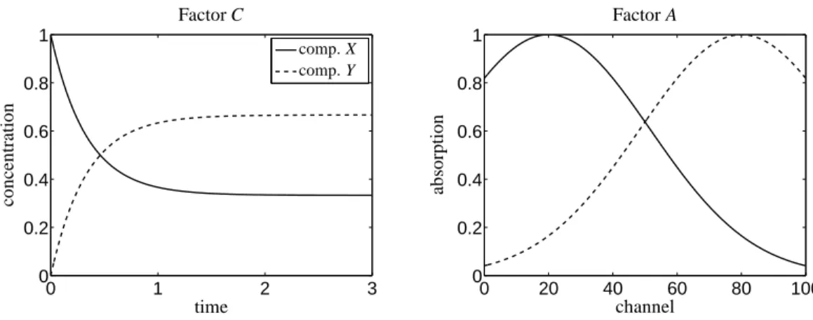
The concentration profiles can be computed by solv- ing the associated initial value problem. The refer- ence reaction rate constants are taken as k∗1 = 2 and k∗
−1=1. For this parametrization the concentration pro- files are shown together with the associated pure com- ponent spectra, two Gaussian functions are assumed, in Figure 3.
First the set of D-consistent rate constantsKis deter- mined. Therefore all 2×2 matrices are to be determined which are similar to M(k). By similarity these matrices have the eigenvalues−k1−k−1and 0. With the trace of a reference matrix M(k∗) withψ=k∗1+k∗
−1, cf. Equation (4.6), this leads to the linear relation
k1+k−1=ψ.
This equation describes a straight line in the positive quadrant of the positive rate constants. In other words k−1=ψ−k1. Hence
K=
( α
ψ−α
!
: α∈(0, ψ]
)
. (6.1)
In order to determine the subsetK+we fix in the present model problem k∗1 = 2 and k∗
−1 = 1 so that ψ = 3, cf. Equation (4.6). By an elimination in the equation CA =CeA which describes two feasible factorizationse (for the details see [27]) we get the subset of rate con- stantsK+being associated with nonnegative A
K+=
( α
ψ−α
!
: α∈[1.9004, ψ]
)
. (6.2) Therein the lower bound forαsatisfies
k1 max
i=1,...,n
A1i−A2i
A1i =1.9004.
The setsKandK+as well as the associated continua of nonnegative factors C and A are shown in Figure 4.
8
0 1 2 3 0
0.2 0.4 0.6 0.8 1
time
concentration
Factor C
comp. X comp. Y
0 20 40 60 80 100
0 0.2 0.4 0.6 0.8 1
channel
absorption
Factor A
Figure 3: Concentration profiles and pure component spectra for the two-component model problem from Section 6.1.
0 1 2 3
0 0.5 1 1.5 2 2.5 3
k1
k−1
The setsKandK+ K K+
0 1 2 3
0 0.2 0.4 0.6 0.8 1
comp. X comp. Y
time
concentration
Factors C
0 20 40 60 80 100
0 0.2 0.4 0.6 0.8 1
channel
absorption
Factors A
Figure 4: The model problem from Section 6.1 is considered. Left: The set of D-consistent rate constantsKby (4.2) is an anti-diagonal broken line and solid line in [0,3]×[0,3]. Its subset of nonnegatively feasible kineticsK+by (4.3) is drawn as a solid line. These sets are analytically given in (6.1) and (6.2). The vector k=(0,3) is not an element ofK; this open end of the set is marked by a small black circle.
Center and right: The continua of associated nonnegative factors C and A for the set of feasible kineticsK+are plotted. A color shading from red to blue is used in order to express the pairing of associated concentration profiles and spectra. The isolated red spectral profile in the right subplot is the spectral profile of X, which can uniquely be extracted from the data at t=0.
9
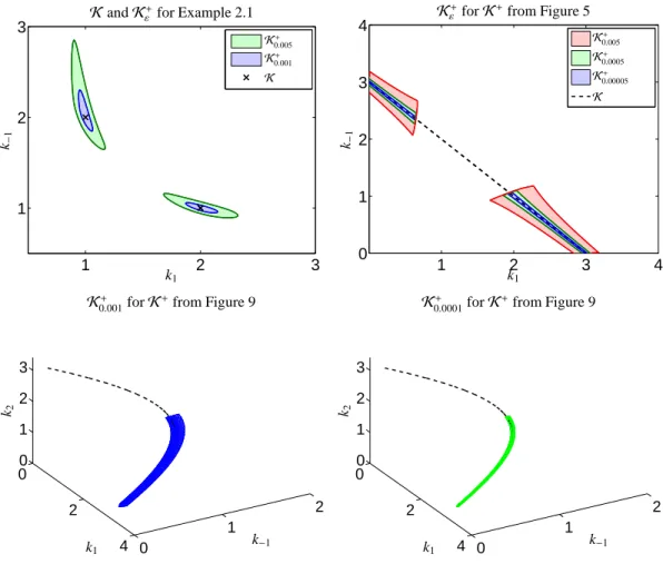
Next the same model problem is considered for non- negative initial concentrations values cX(0) > 0 and cY(0) > 0. Then the subsetK+ ofK consists of two isolated line segments, see Figure 5.
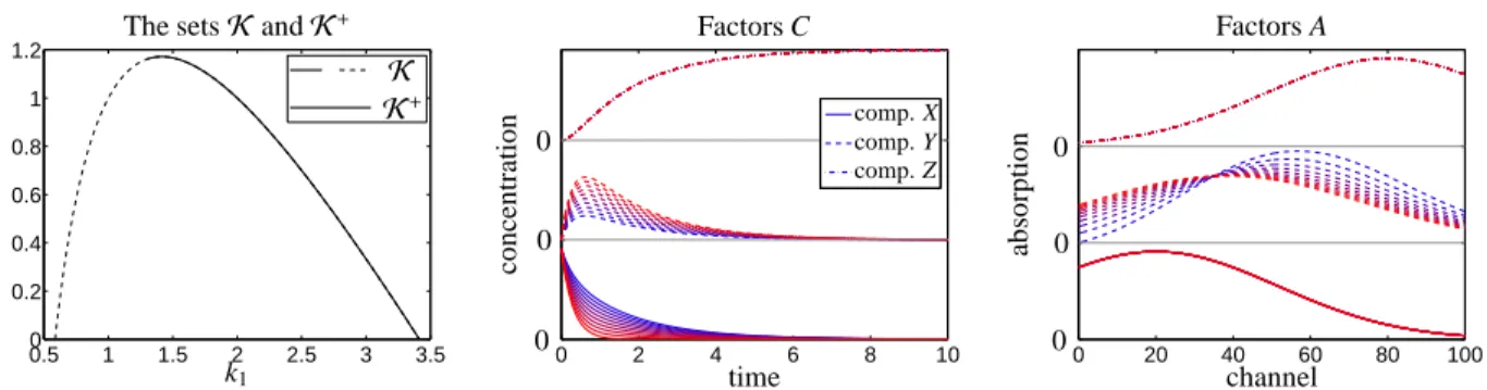
6.2. A three-component partially reversible reaction system - part 1
The reaction mechanism for a three-component sys- tem is taken as follows
X−→k1 Y−−↽k⇀−−2
k−2
Z.
The initial concentrations are given by cX(0) = 1, cY(0)=0 and cZ(0)=0, and the Kirchhoffmatrix reads
M(k)=
−k1 0 0 k1 −k2 k−2
0 k2 −k−2
.
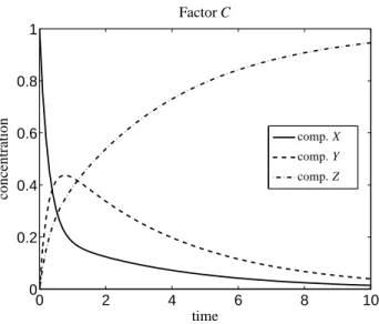
The eigenvalues of the matrix M(k) are λ1 = −k1, λ2 =−k2−k−2andλ3 =0. For the model problem the reference values k∗1 =1, k∗2 =2 and k∗
−2 =1 are used.
For these parameters the concentration profiles and the pure component spectra (three Gaussians) are presented in Figure 6.
The set of D-consistent rate constantsKand its sub- set of feasible rate constants K+ have the following forms
K=
φ α ψ−φ−α
:α∈(0, ψ−φ]
∪
ψ−φ
β φ−β
:β∈(0, φ]
K+=
φ α ψ−φ−α
:α∈[1.7155, ψ−φ]
∪
ψ−φ
β φ−β
:β∈[0.8087, φ]
(6.3) withφ = k∗1 = 1 and ψ = k∗1 +k∗2 +k∗
−2 = 4. The lower bounds forαandβinK+result from a numerical evaluation of the following terms
k2 max
i=1,...,n
A2i−A3i
A2i
=1.7155, k1 max
i=1,...,n
(ψ−k1)A1i+(k1−k−2)A2i−k2A3i k1A2i+(ψ−k1)A1i
=0.8087.
The derivation of these formula requires complex math- ematical computations which have been done by using computer algebra systems; all results have been con- firmed numerically by means of the grid search proce- dure. The setKand its subsetK+of feasible rate con-
stants are plotted in Figure 7. These sets can be plot- ted in 2D as the fixed trace condition, see Section 4.3, implies the linear relation k1 = ψ−k2−k−2 wherein the constant ψ = 4 is the sum of the components of k∗ = (1,2,1). Figure 7 additionally shows the con- tinua of the concentration profiles and of the nonneg- ative spectra which are represented byK+.
6.3. A three-component partially reversible reaction system - part 2
As a second reaction mechanism for a three- component system we consider
X−−↽k⇀−−1
k−1
Y −→k2 Z
with the initial concentrations cX(0)=1, cY(0)=0 and cZ(0)=0. The Kirchhoffmatrix is given by
M(k)=
−k1 k−1 0 k1 −k−1−k2 0
0 k2 0
. Its eigenvalues areλ1,2=−(ψ±√
φ)/2 andλ3=0 with ψ=k1+k−1+k2, φ=(k1+k−1+k2)2−4k1k2. We use the reference values k∗1 =2, k∗
−1 =k∗2 =1. The three pure component spectra for X, Y and Z are the same as used in Section 6.2, see Figure 6. The concen- tration profiles are presented in Figure 8.
The setsK andK+have the form K =
α β(α) γ(α)
: α∈
"
ψ− √ φ 2 ,ψ+√
φ 2
#
, K+=
α β(α) γ(α)
: α∈
"
1.3001,ψ+√ φ 2
#
.
(6.4)
Therein the functionsβ(α) andγ(α) are given by β(α)=−1
4
(ψ−2α)2−φ
α , γ(α)=ψ−α−β(α)
withψ =4,φ =8 and the given values for k∗
±1and k2∗. The lower bound forαinK+has the form
k1 max
i=1,...,n
A1i−A2i
A1i
=1.3001.
All these results together with the continua of nonneg- ative factors C and A which are represented by the set K+of feasible rate constants are presented in Figure 9.
10
0 0.5 1 1.5 2 2.5 3 0
0.5 1 1.5 2 2.5 3
k1
k−1
The setsKandK+
K K+
Figure 5: The model problem from Section 6.1 is considered for the case of nonnegative initial concentrations cX(0)=0.55 and cY(0)=0.45.
Once again the set of D-consistent rate constantsKand also the set of feasible rate constantsK+are shown. The setK+consists of two isolated line segments.
0 2 4 6
0 0.2 0.4 0.6 0.8 1
time
concentration
Factor C
comp. X comp. Y comp. Z
0 20 40 60 80 100
0 0.2 0.4 0.6 0.8 1
channel
absorption
Factor A
Figure 6: Concentration profiles and spectra of the pure components for the model problem from Section 6.2. The reaction rate constants are k1=1, k2=2 and k−2=1, and the initial concentrations are set to cX(0)=1, cY(0)=0 and cZ(0)=0.
0 1 2 3
0 0.5 1 1.5 2 2.5 3
k2
k−2
The setsKandK+ K K+
0 2 4 6
comp. X comp. Y comp. Z
time
concentration
Factors C
0 0 0
0 20 40 60 80 100
channel
absorption
Factors A
0 0 0
Figure 7: Analysis of the three-component model system from Section 6.2. Left: The set of D-consistent rate constantsKis drawn by dashed and by solid lines. Its subsetK+is plotted by the solid line. All these lines are open at k2 = 0, i.e. the points (k1,k2,k−2) = (3,0,1) and (k1,k2,k−2)=(1,0,3) do not belong toK. These two points are marked by small circles. Because of the fixed trace condition, see Section 4.3, and k1=4−k2−k−2for k∗=(1,2,1), the setsKandK+can be drawn in 2D.
Center and right: The continua of associated nonnegative factors C and A for the set of feasible kineticsK+are plotted. A color shading from red to blue is used in order to express the pairing of associated concentration profiles and spectra. The single/isolated concentration profiles or spectra represent unique solutions, e.g. the spectral profile of X can uniquely be extracted from the data at t=0.
11
0 2 4 6 8 10 0
0.2 0.4 0.6 0.8 1
comp. X comp. Y comp. Z
time
concentration
Factor C
Figure 8: The concentration profiles for the three-component model system from Section 6.3. The pure component spectra are the same as used in Section 6.2 and are shown in Figure 6.
0.5 1 1.5 2 2.5 3 3.5
0 0.2 0.4 0.6 0.8 1 1.2
k1
k−1
The setsKandK+ K K+
0 2 4 6 8 10
comp. X comp. Y comp. Z
time
concentration
Factors C
0 0 0
0 20 40 60 80 100
channel
absorption
Factors A
0 0 0
Figure 9: Analysis of the three-component model system from Section 6.3. Left: The set of D-consistent rate constantsKis drawn by dashed and by solid curved lines. Its subsetK+is plotted by the solid line. These sets are given analytically in Equation (6.4). Because of the fixed trace condition, see Section 4.3, and k2=4−k1−k−1, the setsKandK+can be drawn in 2D.
Center and right: The continua of associated nonnegative factors C and A are plotted for the set of feasible kineticsK+. A color shading from red to blue is used in order to express the pairing of associated concentration profiles and spectra. The pure component spectra of X and Z are known (from the spectral data at t=0 and t=10). Then the complementarity theory [28, 29, 30] guarantees that the concentration profile of the complementary component Y is also uniquely determined aside from scaling; and in fact, the continuum of concentration profiles of Y is spanned by a single function and its scalar multiples.
12
6.4. A three-component system including parallel reac- tions
Next the three components X, Y and Z are assumed to form two reaction pathways for the component X. The reaction mechanism is
X−−↽k⇀−−1
k−1
Y, X−→k2 Z
with the initial concentrations cX(0)=1, cY(0)=0 and cZ(0)=0. Hence the Kirchhoffmatrix reads
M(k)=
−k1−k2 k−1 0 k1 −k−1 0
k2 0 0
. The eigenvalues of M(k) areλ1,2=−(ψ±√
φ)/2,λ3=0 with
ψ=k1+k−1+k2,
φ=(k1+k−1+k2)2−4k−1k2.
The reference values for the rate constants are taken as k1∗ =2 and k∗−1 =k∗2 =1. Once again, the same Gauss profiles as used in Section 6.2 are taken for the pure component spectra. The solution of the initial value problem (2.1) with the present M(k) and the given ini- tial values results in the concentration profiles which are shown in Figure 10.
The set of D-consistent rate constantsKand its sub- set of nonnegatively feasible rate constantsK+read
K =
α(β)
β γ(β)
: β∈
"
ψ−√ φ 2 ,ψ+ √
φ 2
!
, K+=
α(β)
β γ(β)
: β∈[0.58115,1.7207]
.
(6.5)
Therein the constantsα(β) andγ(β) are given by α(β)=−1
4
(ψ−2β)2−φ
β , γ(β)=ψ−α(β)−β
andψ = 4, φ = 12. The analytic formula for theβ- interval inK+are skipped due to their high complexity.
Instead, only the numerical evaluation of these bounds is given. Figure 11 shows the setsK andK+together with the associated continua of nonnegative feasible fac- tors C and A.
6.5. Feasible rate constants for perturbed/noisy experi- mental data
Next the set of feasible rate constants is computed for UV/Vis data from [31] where the influence of sub- stituents in ButiPhane ligands is investigated on the hy- drogenation activity of rhodium complexes. A number of k=82 UV/Vis spectra each with n=1951 channels is given. The underlying reaction mechanism is simply X −→k1 Y. In order to demonstrate the computation of the set of feasible rate constants we assume the slightly more complex mechanism of the equilibrium
X−−↽k⇀−−1
k−1
Y.
The set of nonnegatively feasible rate constantsKε+with respect to the noise levelε ≥0 is computed, cf. (5.1).
The following analysis allows to judge of the question whether or not the experimental data could also be in- terpreted by an equilibrium reaction.
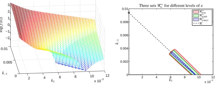
Due to the high quality of the UV/Vis spectral data only a relatively small noise levelεis assumed. For the given experimental data we have observed the minimum minkf (k)=1.09·10−5. This shows thatεmust be larger than 1.09·10−5 in order to find any feasible solutions.
First the function f (k) is evaluated on the rectangle of reaction rate constants
(k1,k−1)∈[10−3,2·10−2]×[0,10−2].
The results and the computed setsKε+for the three dif- ferent valuesε∈ {1.5·10−3,5·10−3,1·10−2}are pre- sented in Figure 12. All computations have been exe- cuted by using a simple grid search method; the com- putational costs for the evaluation of the cost function are not very high. As the set Kε+consists only of one connected set, even the polygon inflation technique [7]
can be used for the numerical computation ofKε+. 6.6. Numerical computation of the setKε+
In Section 5.1 the setKε+of feasible rate constants for perturbed data is introduced. By definition it holds that
K+⊂ Kε+⊆ Kε˜+
for every 0≤ε≤ε.˜
First, we consider Example 2.1 for which the setK+ consists of only two isolated points. For the two noise levels
ε∈ {1·10−3,5·10−3}
the two setsKε˜+increase aroundK+, which is shown in the upper left sub-plot of Figure 13. For this problem 13
0 2 4 6 8 10 0
0.2 0.4 0.6 0.8 1
comp. X comp. Y comp. Z
time
concentration
Factor C
Figure 10: The concentration profiles for the three-component model data from Section 6.4. The pure component spectra are the same as used in Section 6.2 and shown in Figure 6.
0 0.5 1 1.5 2
0 1 2 3 4
k1
k−1
The setsKandK+ K K+
0 2 4 6 8 10
comp. X comp. Y comp. Z
time
concentration
Factors C
0 0 0
0 20 40 60 80 100
channel
absorption
Factors A
0 0 0
Figure 11: Analysis of the three-component model system including parallel reactions from Section 6.4. Left: The set of D-consistent rate constantsKis drawn by dashed and by solid lines. Its subsetK+is plotted by the solid line. Because of the fixed trace condition, see Section 4.3, and k2=4−k1−k−1for k∗=(2,1,1), the setsKandK+can be drawn in 2D.
Center and right: The continua of associated nonnegative factors C and A for the set of feasible kineticsK+are plotted. A color shading from red to blue is used in order to express the pairing of associated concentration profiles and spectra. The single/isolated spectra represent unique solutions.
14