Reduction of the rotational ambiguity of curve resolution techniques under partial knowledge of the factors. Complementarity and coupling theorems.

(1)

Reduction of the rotational ambiguity of curve resolution techniques under partial knowledge of the factors. Complementarity and coupling theorems.

Mathias Sawall^a, Christian Fischer^b, Detlef Heller^b, Klaus Neymeyr^∗a

aUniversit¨at Rostock, Institut f¨ur Mathematik, Ulmenstrasse 69, 18057 Rostock, Germany

bLeibniz-Institut f¨ur Katalyse, Albert-Einstein-Strasse 29a, 18059 Rostock

Abstract

Multivariate curve resolution techniques allow to uncover from a series of spectra (of a chemical reaction system) the underlying spectra of the pure components and the associated concentration profiles along the time axis. Usually a range of feasible solutions exists due to the so-called rotational ambiguity. Any additional information on the system should be utilized to reduce this ambiguity.

Sometimes the pure component spectra of certain reactants or products are known or the concentration profiles of the same or other species are available. This valuable information should be used in the computational procedure of a multivariate curve resolution technique.

The aim of this paper is to show how such supplemental information on the components can be exploited. The knowledge of spectra leads to linear restrictions on the concentration profiles of the complementary species and vice versa. Further affine linear restrictions can be applied to pairs of a concentration profile and the associated spectrum of a species. These (affine) linear constraints can also be combined with the usual non-negativity restrictions. These arguments can reduce the rotational ambiguity considerably. In special cases it is possible to determine the unknown concentration profile or the spectrum of a species only from these constraints.

Key words: chemometrics, factor analysis, pure component decomposition, non-negative matrix factorization, spectral recovery.

1. Introduction

The aim of a model-free pure component decomposition is to extract the pure component spectra and the associated concentration profiles from the series of spectra of the (chemical reaction) system. In the best case no additional information is used for this computational procedure; even the number of reacting species is a result.

Typically the spectroscopic data is provided on a frequency×time grid in the form of a matrix; this data matrix is denoted by D. Due to the Lambert-Beer law a factorization of D into matrix factors C and A is de- sired, where C column-wise contains the concentration profiles and A row-wise contains the pure component spectra (molar extinction coefficients). As C and A are non-negative matrices, the pure component decomposition can be considered as the problem of the computation of a non-negative matrix factorization. However, this mathematical problem (aside from singular excep- tional cases) turns out to have a continuum of possible

solutions. Most of these solutions do not have a chemical/physical meaning or importance and should be dis- regarded. These (so-called) abstract factors constitute a considerable obstacle for a fast and stable (hard) model- free pure component decomposition. There is a vast lit- erature on these methods, see e.g. [17, 18] and the references therein.

Often some additional facts on the chemical reaction system are known. Sometimes the number of starting reactants is given and/or some of their pure component spectra are available. Further the spectra of the main products might be accessible or even those of interme- diary products. All these data reduce the set of the mathematically feasible factorizations to those factorizations which are consistent with the pre-given supplemental data.

The goal of this paper is a systematic analysis of the relation between such supplemental data and the resulting constraints on the set of feasible solutions in order to extract the relevant and chemically meaningful solutions. We derive the results (in the form of a couple of

∗Correspondence to: K. Neymeyr, Universit¨at Rostock, Institut f¨ur Mathematik, Ulmenstrasse 69, 18057 Rostock, Germany. June 10, 2012

(2)

theorems) by combining the Lambert-Beer law with a singular value decomposition (SVD) of the data matrix D. To this end we apply various arguments from lin- ear algebra to the columns of the concentration matrix C and rows of the absorption matrix A.

The paper is organized as follows. In Section 2 the problem of a pure component decomposition is intro- duced and classical approaches to its solution are presented. Some comments on the enclosure of the range of admissible solutions follow in Section 3. Section 4 contains the main mathematical results. These results are linear constraints on “complementary species” and also affine linear constraints coupling the spectrum and the concentration profile for particular species. All these restrictions are combined with the typical non-negativity constraints. To demonstrate the usefulness of the arguments we apply the theorems to a three-component model problem in Section 5. Further a three-component reaction system which results in the formation of hafnacyclopentene is analyzed in Section 6.

2. Self-modeling curve resolution

The Lambert-Beer law only holds in the absence of error sources like noise and nonlinearities. Its perturbed form reads

D=CA+E.

The data matrix D∈R^k×ncontains in its rows k spectra (taken at different times from a chemical reaction sys- tem); each spectrum is given at n frequencies (or spec- tral channels). If the reaction system contains s species, then the concentration matrix C ∈ R^k×s contains in its s columns the concentration profiles. The matrix A∈R^s×nholds the associated s pure component spectra in the rows. The error matrix E ∈ R^k×n comprises the mentioned deviations from the linear Lambert-Beer law.

The problem of a self-modeling curve resolution technique (hard model-free analysis) is to compute only from the given matrix D the number of species s to- gether with proper matrix factors C and A in such a way that the error matrix D−CA is close to the zero matrix. For such hard model-free methods we refer to [16, 17, 18] and the references therein.

2.1. The mathematical factorization problem

Mathematically the (hard) model-free analysis in absence of error terms is a factorization problem for the matrix D. The factors C and A are non-negative matri- ces. We refer to this problem as

Problem 2.1 (Non-negative matrix factorization). For D∈R^k×n+ with rank(D)=s the problem is to find non- negative matrix factors so that

D=CA (1)

with C∈R^k×s+ and A∈R^s×n+ .

Therein the rank s of D equals the number of columns of C and the number of rows of A. Problem 2.1 is a so-called inverse problem. It is well known that an ar- bitrary non-negative k×n matrix D with 2<rank(D)<

min(k,n), and hence min(k,n)>3, may have no factorization of the form (1); for a discussion of the existence and uniqueness of solutions, see [5, 6, 33, 34]. For spec- tral data matrices D the existence of an “approximate”

factorization (1) can be assumed, since D (due to the Lambert-Beer law) originates from the physical quanti- ties which are inscribed into the matrix factors C and A.

The factorization “reverses” the physics of the problem.

However, problem 2.1 usually has a continuum of possible solutions. The insertion of an invertible ma- trix T ∈ R^s×s and its inverse in (1) results in a further factorization

D=(CT⁻¹) (T A). (2)

If these transformed factors CT⁻¹ and T A are non- negative matrices (which can be achieved for proper T ), then a further mathematically feasible solution is found.

Typically the factorization problem does not have a unique solution due to the rotational ambiguity induced by T . We ignore the trivial non-uniqueness which orig- inates from permuted diagonal matrices T , since such matrices correspond to positively scaled and reordered solutions. On the uniqueness question see Manne’s theorems [20], Malinowski [19] and the work of Rajk ´o [29]

together with the references therein. For the mathematical background of this problem see e.g. [7, 31]. To find the correct and chemically relevant solution within the set of (mathematically) feasible solutions one can try to compute or to characterize the whole set of feasible solutions [9, 10, 16, 25]. Then one hopes to detect the desired solution within this set. Alternatively, one can apply proper regularizations to the factorization problem and hopes to steer the factorization procedure in the correct direction [18, 22, 23, 36].

In any case the first step of the computational process is the construction of a truncated singular value decom- position to construct a basis for the factors C and A.

This is the classical approach of Lawton and Sylvestre [16].

2

(3)

2.2. Factorization by the singular value decomposition The singular value decomposition (SVD) [11] for a given D∈R^k×nreads

D=UΣV^T

with orthogonal matrices U ∈R^k×kand V ∈R^n×n. The diagonal matrixΣ∈R^k×n

Σi,j=

( σi for i= j, 0 for i, j,

contains the non-negative singular valuesσiin decreas- ing order with i.

If D has the rank s, then the SVD can be reduced to D=U ˜˜ΣV˜^T (3) where ˜U is a submatrix of U which contains the s left singular vectors being associated with the non-zero singular values. Further ˜V is built from the associated s right singular vectors and ˜Σis the leading s×s subma- trix of ˜Σ.

The SVD provides a factorization of D. In the con- text of a self-modeling curve resolution technique ˜U ˜Σ and ˜V^T are called abstract factors; these factors usually contain negative components and cannot be used for a chemical/physical interpretation. The trick from (2) to introduce a proper transformation matrix and its inverse is decisive for a successful solution of the reconstruction problem; see, among many others, the references [1, 10, 16, 18, 22, 35]. By means of a proper T ∈R^s×s it is possible to recover the factors C and A as follows

D=U ˜˜ΣT⁻¹

| {z }

C

T ˜V^T

|{z}

A

. (4)

Thus the aim of a self-modeling curve resolution (SMCR) technique is to construct just such a suitable transformation matrix T .

3. Enclosure of solutions

The rotational ambiguity of the factors C and A is an annoying fact which complicates the development of universal and stable SMCR algorithms. The computational (and sometimes analytical) determination of the range of feasible solutions can help in the analysis of chemical reaction systems. Here a brief overview is given on classical and more recent analytical and numerical techniques on the enclosure of feasible solutions; these techniques are essentially based on the required non-negativity of the solutions.

3.1. Enclosure of feasible solutions

The range of admissible solutions for a two- component (s = 2) system has partly been analyzed analytically by Lawton and Sylvestre [16]. This work is among the earliest “chemometric” publications. Fur- ther Maeder and his coworkers contributed to this topic [1, 35]; see also the papers of Rajk ´o and Istv´an [28, 30].

For dimensions s > 2 a comparable analysis gets much harder. For three-component systems Borgen et al. did pioneering work [3, 4]. Rajko et al. improved the analytical solution for three-component systems with computer geometry tools (Borgen plots), see [26, 27]

and the references in these papers. A novel approach to compute the boundaries of the set (or manifold) of solutions for three-component systems has been presented by Golshan, Abdollahi and Maeder in 2011 [10].

In some of these works the Perron-Frobenius theorem [21] appears as an important tool. This theorem characterizes the largest eigenvalue (singular value) and the associated singular vector of a non-negative matrix.

Boundaries for the range of possible solutions can be derived by determining all transformations of the first two (or three) right singular vectors which result in non- negative spectra. The associated inverse transformations can be applied to the left singular vectors and must also result in non-negative concentration profiles. This approach has been used e.g. in [10, 16] to construct op- timal factors C and A which also fulfill D≈CA.

However, various other hard and soft constraints can be applied. Sometimes even a pre-given kinetic model can be used for the regularization of the optimization procedure. This allows to find optimal kinetic constants by a kinetic regularization together with optimized C and A simultaneously, see [12, 14, 32].

3.2. Usage of supplementary information

Self-modeling curve resolution techniques are hard model-free methods in a sense that no a-priori informa- tion on the chemical system is needed for the construc- tion of the factors C and A. However, sometimes certain information on the system is available, e.g., some of the pure component spectra of the starting reactants or of certain products may be known from separate measure- ments. Further the number of starting reactants or products may be given. Such additional information on the system should be utilized in order to reduce the range of admissible non-negative factorizations. This data can be used as a hard (or even soft) constraint on C and A while minimizing the reconstruction error D−CA. A mathematical approach of how to exploit such information in the computational procedure is presented in the next section.

3

(4)

4. Reduction of the rotational ambiguity

As explained in Section 3 any additional information on the chemical reaction system can be exploited to reduce the rotational ambiguity of the solutions of a self- modeling curve resolution technique. Next we use arguments of linear algebra to prove

1. the complementarity theorem 4.2 which allows to impose restrictions on the concentration profiles of complementary species if certain spectra are given (and vice versa),

2. the coupling theorems 4.5 and 4.6 which prove affine linear constraints for pairs of a spectrum and the associated concentration profile,

3. a non-negativity theorem 4.7 which provides ad- missible ranges for the components that can be derived from the non-negativity constraints.

In this section we assume the Lambert-Beer law to hold exactly, i.e., D is given as the exact product of C and A. Hence we ignore any nonlinearities and error terms. Therefore the existence of a solution of Problem 2.1 is guaranteed. The results of this section can be applied to practical data (containing error terms), which is shown in Section 6. However, with a decreasing signal- to-noise ratio the application of the results gets harder.

It is worth to note that the complementarity-coupling theorems are different from the duality results as in- troduced by Henry [13] for multivariate receptor modeling and discussed by Rajk ´o [24] in the SMCR con- text. This duality approach uses the non-negativity constraints to find restrictions on the feasible regions and works with the ”external” matrices ˜U and ˜V in (4). In contrast to this, the complementarity-coupling approach is based on the partial knowledge of the factors C or A and uses the coupling through the ”inner” matrix pair T and T⁻¹ in (4) in order to derive restrictions on the feasible regions. The mathematical arguments also rely on rank/dimension arguments which are combined with non-negativity constriants.

4.1. The colon notation

A useful notation to specify a row or a column of a matrix is the colon notation. For a matrix M∈R^n×mits kth row is denoted by

M(k,:)=(mk1, . . . ,mkm) and its kth column is

M(:,k)=





 m_1k

... mnk





 .

Further, we use the colon notation to extract sub- matrices. If 1 ≤ i1 ≤ i2 ≤ n and 1 ≤ j1 ≤ j2 ≤ m, then M(i₁: i₂,j₁: j₂) is the submatrix of M which results from extracting the rows i₁ through i₂and the columns

j1through j2. For example one gets

M(3 : 4,2 : 5)= m32 m33 m34 m35

m42 m43 m44 m45

! .

The n-by-n identity matrix is denoted by I_nwith In=(e1, . . . ,en)

where ekis the standard basis vector ek=( 0, . . . ,0

| {z }

(k−1)−times

,1, 0, . . . ,0

| {z }

(n−k)−times

)^T. (5)

Sub-matrices of the identity matrix can be used to ex- tract sub-matrices of M in the following way

M(:,k : l)=M I(:,k : l) and M(k : l,:)=I(k : l,:) M.

In words, the right-multiplication with I(:,k : l) extracts columns from M and left-multiplication with I(k : l,:) extracts rows from M.

4.2. The complementarity theorem

Next we consider the situation that one (or even more than one) of the pure component spectra are known. A typical case is that these known spectra are those of the reactants of the chemical reaction; sometimes the spectra of certain products are also given. This supplementary knowledge of the chemical system should be exploited within the computation of the pure component factorization of D. Theorem 4.2 shows that such addi- tional information on the columns of A imposes restric- tions on the complementary columns of the concentra- tion matrix C. These restrictions are expressed in the form of linear equations and can be used to reduce the rotational ambiguity of the decomposition.

The special case that s−1 pure component spectra are known within an s-component system is discussed in Corollary 4.3. For this problem the complementarity principle shows that the concentration profile of the single remaining component is unique (aside from scaling).

In Sec. 4.3 further theorems are proved, which characterize the concentration profiles of the same species for which the spectra are available.

Lemma 4.1 proves an auxiliary result which is required for the proof of Theorem 4.2.

4

(5)

Lemma 4.1. Let T ∈R^s×sbe a regular matrix and 1≤ s0<s. Then

T (1 : s₀,:)y=0 holds if and only if y∈R^sis of the form

y=T⁻¹(:,s0+1 : s)z for a proper z∈R^s−s⁰.

Proof. Any regular matrix T satisfies T T⁻¹=I.

Left-multiplication of this equation with I(1 : s0,:) ex- tracts the first s0 rows and right-multiplication with I(:,s0+1 : s) extracts the last s−s0columns so that

T (1 : s0,:)T⁻¹(:,s0+1 : s)=0∈R^s⁰^×s−s⁰, (6) i.e. the s0×s−s0zero-matrix.

If y = T⁻¹(:,s0+1 : s)z with z ∈ R^s−s⁰, then left multiplication with T (1 : s0,:) together with (6) yield

T (1 : s0,:)y=T (1 : s0,:)T⁻¹(:,s0+1 : s)z=0z=0.

To prove the other direction just observe that the columns of T⁻¹(:,s₀+1 : s) build a basis of the null space of T (1 : s₀,:). This argument reads in detailed form as follows: LetN be the null space (or kernel) of T (1 : s0,:) ∈ R^s⁰^×s, i.e. any y ∈ N satisfies T (1 : s0,:)y =0 and vice versa. As T is a regular ma- trix the rank of its submatrix T (1 : s0,:) is s0 and the dimension of its null spaceNequals s−s0.

Further the dimension of the column space (or image) Mof T⁻¹(:,s0+1 : s) equals s−s0(once again due to the regularity of T ).

Equation (6) proves thatMis a subspace ofN and dimM=dimN proves thatM=N. Thus any y∈ N with T (1 : s₀,:)y=0 can be represented by a z∈ R^s−s⁰ so that y=T⁻¹(:,s₀+1 : s)z.

The central theorem is as follows; thereinR^n×m+ de- notes the set of n-by-m real matrices with non-negative entries.

Theorem 4.2. Let D ∈ R^k×n+ with rank(D) = s be de- composable in a way that D=CA with C ∈ R^k×s+ and A∈ R+^s×n. The truncated singular value decomposition of D, see (3), reads D = U ˜˜ΣV˜^T with ˜U and ˜V having the rank s.

We assume that s₀rows (i.e., s₀spectra) of the factor A are known with s₀ < s. Without loss of generality these known spectra can be placed in the first s0rows of A. Thus A(1 : s0,:)∈R^s⁰^×nis given.

Then the complementary columns C(:,i), i = s0 + 1, . . . ,s, of C are contained in the (s−s0)-dimensional vector space

{U ˜˜Σy : y∈R^s with A(1 : s0,:) ˜V y=0}, (7) which is a linear subspace of theR^k. (In words (7) de- fines the set of all vectors ˜U ˜Σy, where y is a vector in theR^ssatisfying A(1 : s0,:) ˜V y =0. Alternatively, one can describe the set (7) as the kernel (null space) of the matrix A(1 : s0,:) ˜V which is multiplied from the left by U ˜˜Σ.)

Proof. A regular matrix T ∈ R^s×sexists which relates the factors in D =CA to the factors in D=( ˜U ˜Σ) ˜V^Tin a way that

C=U ˜˜ΣT⁻¹ and A=T ˜V^T; for a proof see, e.g., Lemma 2.1 in [22].

The pre-given first s0rows of A can be written as I(1 : s0,:) A=A(1 : s0,:)=T (1 : s0,:) ˜V^T. Right multiplication with ˜V yields

A(1 : s0,:) ˜V=T (1 : s0,:) ˜V^TV˜=T (1 : s0,:) (8) so that the first s0rows of T are also known.

Further from C = U ˜˜ΣT⁻¹ we get for its s−s0 last columns

C(:,s₀+1 : s)=C I(:,s₀+1 : s)=U ˜˜ΣT⁻¹(:,s₀+1 : s).

The image (or column space) of this matrix is I={U ˜˜ΣT⁻¹(:,s0+1 : s)z for z∈R^s−s⁰}.

Lemma 4.1 allows to rewrite this space as

I={U ˜˜Σy : with y∈R^sso that T (1 : s₀,:)y=0}.

Insertion of (8) allows to eliminate T (1 : s0,:) and

proves the proposition.

Next we consider the extremal case that s0 = s−1.

This means that only one pure component spectrum is unknown. Then Theorem 4.2 shows that the concentration profile of this single component is uniquely determined (aside from scaling).

Corollary 4.3. On the assumptions of Theorem 4.2 as- sume the first s−1 rows of A to be given. Then the com- plementary concentration profile C(:,s) is unique (aside from scaling).

5

(6)

Proof. The (s−1×s)-matrix A(1 : s−1,:) ˜V has the maximal rank s−1 since rank(D) = s. Hence its null space is a one-dimensional space and has the form{ty : t ∈R}for a proper y,0. Theorem 4.2 shows that the concentration profile reads C(:,s)=U ˜˜Σyt with a proper

scaling constant t∈R.

Remark 4.4. The complementarity theorem 4.2 can also be formulated for pre-given columns of C and the resulting implications on the complementary rows of A.

This means that for known concentration profiles (i.e., some of the columns of C are given) the spectra of the complementary species are characterized by a condition like (7). The direct pendant of Corollary 4.3 reads as follows: If (for some reason) the concentration profiles of s−1 components are available, then the spectrum of the single remaining species is uniquely determined (aside from non-negative scaling).

4.3. The coupling theorems

In Sec. 4.2 we have analyzed the way in which the knowledge of s0 spectra imposes restrictions on the concentration profiles of the complementary species in- dexed with s0 +1, . . . ,s. Next we analyze the way in which the knowledge of certain pure component spectra affects the concentration profiles of just the same species. This analysis results in affine-linear constraints which are formulated in the coupling theorem 4.5. Ad- ditionally, the non-negativity constraints can be used to formulate further restrictions (in order to reduce the rotational ambiguity); this is the topic of Sec. 4.4.

The theorem (once again) exploits the relation of the pure component factorization of D with the truncated singular value decomposition (4). The key observation is that the “subtraction” of a single component from the system can be represented by

D−C(:,i)A(i,:),

where C(:,i)A(i,:) is a dyadic product with the rank 1.

If A(i,:) is known, then the correct concentration profile C(:,i) as an element from the column space of D satis- fies the constraint rank(D−C(:,i)A(i,:))=s−1, since the subtraction of C(:,i)A(i,:) “removes” the ith species from the system. In other words the rank reduction by 1 is a constraint on the unknown profile C(:,i).

Theorem 4.5. Let D ∈ R^k×n+ with rank(D) = s be decomposable so that D = CA with C ∈ R^k×s+ and A ∈ R^s×n+ . Let ˜U ˜ΣV˜^T be a truncated singular value decomposition of D.

If the ith row of A is known, then the associated col- umn C(:,i) is an element of the (s−1)-dimensional affine-linear space

{U ˜˜Σy : y∈R^s with A(i,:) ˜Vy−1=0} ⊂R^k. (9) Proof. The proof is similar to that of Theorem 4.2. The ith row of matrix T is known since T (i,:) = A(i,:) ˜V.

The ith diagonal element of T T⁻¹ = I is T (i,:)T⁻¹(:

,i) =1. Hence A(i,:) ˜VT⁻¹(:,i) =1. Therefore the ith column vector T⁻¹(:,i) is an element of the affine-linear space {y ∈ R^s : A(i,:) ˜Vy = 1} with the dimension s−1. Since C(:,i) = U ˜˜ΣT⁻¹(:,i) the affine space of admissible solutions C(:,i) has the form{U ˜˜Σy : y ∈ R^s, A(i,:) ˜Vy−1=0}which is a subset of theR^k. This theorem can also be formulated in a form which treats the case that s0 ≥1 pure component spectra are known. Then the space of admissible concentration pro- files is an (s−s0)-dimensional subspace. This form of the Theorem 4.5 is similar to Theorem 4.2.

Theorem 4.6. Let D∈R^k×n+ with rank(D)=s which is decomposable in D=CA with C∈R^k×s+ and A∈R+^s×n. Let ˜U ˜ΣV˜^T be the truncated singular value decomposi- tion of D. We assume that the first s₀ rows of A are known.

Then for each i, i=1, . . . . ,s0, it holds that the con- centration profile C(:,i) is contained in the affine-linear vector space

{U ˜˜Σy : y∈R^s,A(1 : s0,:) ˜Vy=ei} ⊂R^k (10) whose dimension is s−s0. Therein ei ∈ R^s⁰is the ith standard basis vector, see (5).

Proof. We proceed as in the proof of Thm. 4.5. How- ever, we consider T ( j,:) = A( j,:) ˜V and we get T ( j,: )T⁻¹(:,i)=0 if j ,i. Therefore, A( j,:) ˜VT⁻¹(:,i) =0.

From this one gets that C(:,i) is an element of {U ˜˜Σy : y ∈ R^s, A( j,:) ˜Vy = 0}. Combining this with the re- sult of Thm. 4.5 shows that A(1 : s0,:) ˜Vy=eiwith the

standard basis vector ei.

4.4. Non-negativity

Let us review what is known on the columns of C and the rows of A. First, by definition, the columns of C are vectors from theR^kand the rows of A are from theRⁿ. Second, the singular value decomposition provides s- dimensional subspaces (namely the column space of ˜U and the column space of ˜V) which contain the desired concentration profiles and spectra. Third, the Theorems 4.2 and 4.5 impose additional constraints on these solutions. These constraints are valuable in order to reduce 6

(7)

the rotational ambiguity, i.e., to reduce the set of admissible factorizations. Sometimes (in favorable cases) certain concentration profiles or spectra are uniquely determined (as in Corollary 4.3).

Additionally, there are the non-negativity constraints on the factors C and A. These constraints can be merged with the spaces given in (7) and (9). Due to the nature of these non-negativity constraints (which imply bounds on the scaling factors) one gets subsets of admissible solutions of the linear and affine-linear spaces (7) and (9). Theorem 4.7 deals with the case of an affine-linear space; in the case of a vector space only (non-useful) lower bounds equal to 0 can be derived.

Theorem 4.7. On the assumptions of Theorem 4.5 let

¯c⁽ⁱ⁾∈R^kbe a vector (of upper bounds for C(:,i)) whose components are defined as

(¯c⁽ⁱ⁾)j:= min

ℓ=1, . . . ,n, Aiℓ>0

Djℓ

Aiℓ

, for j=1, . . . ,k.

Then the set (9) of admissible concentration profiles can be reduced to

{U ˜˜Σy : y∈R^swith A(i,:) ˜Vy=1

and 0≤U ˜˜Σy≤¯c⁽ⁱ⁾}. (11) In (11) the vector inequalities are to be interpreted component-wise.

Proof. The matrices C and A are component-wise non- negative. Therefore for all j, ℓ,i it holds that

CjiAiℓ ≤ Xs

k=1

CjkAkℓ=Djℓ,

which implies Cji≤Djℓ/Aiℓif Aiℓ,0. Thus

Cji≤ min

ℓ=1, . . . ,n, Aiℓ>0

Djℓ

Aiℓ

, i=1, . . . ,k. (12)

The right-hand side defines the upper bound (¯c⁽ⁱ⁾)j. The- orem 4.5 provides the space (9) of possible solutions for the concentration profiles C(:,i). The combination of the bound (12) with (9) proves the proposition.

Theorem 4.7 can be generalized to the case that sev- eral spectra are known; this can be stated in a form similar to Theorem 4.6.

4.5. Noisy data and perturbations

The analytical results of this section have been derived on the assumption of the idealized pure compo- nent decomposition D = CA. However, for any prac- tical spectroscopic data matrix D nonlinearities and er- rors of the measurement result in a perturbed factoriza- tion problem D = CA+E. For such a problem not only the factors C and A are to be determined but also a small perturbation matrix E is desired, i.e., E should be close to the zero-matrix. The reconstruction problem with pre-given (known) spectra is stable as long as these spectra can be well constructed from the right singular vectors, i.e., the errorkA(i,:)−A(i,:) ˜V ˜V^Tkis small.

Moreover, ˜U ˜ΣV˜^Thas to be a good approximation of D, which means that the singular valueσs+1is small com- pared toσ1, . . . , σs. If this is the case, then the singular vectors corresponding to the s largest singular values al- low a good approximation of the linear and affine-linear subspaces which are determined in the Theorems 4.2 and 4.5. According to our experience difficulties may occur in the application of the interval restrictions (11) to noisy data. Such problems appear if for a given spec- trum A(i,:) and for certain l both Ai jand Dilare close to zero.

5. A three-component model problem

In this section we apply the theoretical results to a three-component (artificial) catalytic model reaction.

We consider the following system of second order reac- tions

X+Y −^k→¹ K, X+K−→^k² 3Y.

(13)

The initial concentrations of the species X, Y and K are the components of the column vector c(0) which is as- sumed as c(0) =(1,0.1,0)^T. The kinetic constants are taken as k1 =0.05, k2 =1. The numerical solution of the initial value problem for t ∈ [0,100] is computed by the ode15s multi-step solver for stiff problems of Matlab. This highly accurate solution is restricted to an equidistant grid with k=101 nodes in [0,100].

The absorption spectra of the three components X, Y and K are taken as linear combinations of Gaussians in 7

(8)

0 50 100 0

0.2 0.4 0.6 0.8 1

replacements

time [s]

c(t)

Concentration profiles

0 100 200 300 400 500 0.5

1 1.5 2 2.5 3

λ

a(λ)

Absorption spectra

0 200 400

0 50 100

1 2 3

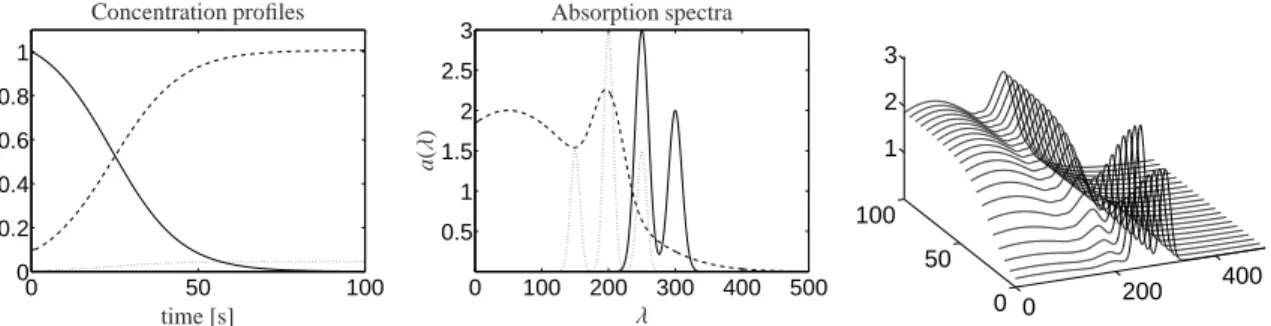
Figure 1: Model problem: concentration profiles with limt→∞c2(t)/c3(t)=21.7577 (left), absorption spectra (center) and mixture spectra (right).

Component X (solid line), component Y (dashed line) and component K (dotted line).

the form (we use the indexes 1,2,3 for X, Y, K) a1(λ)=3 exp(−(λ−250)²

200 )+2 exp(−(λ−300)² 200 ), a2(λ)=2 exp(−(λ−50)²

30000 )+1.3 exp(−(λ−200)² 1000 ), a3(λ)=3 exp(−(λ−200)²

100 )+3

2exp(−(λ−250)²

100 )

+3

2exp(−(λ−150)²

100 )

withλ ∈ [0,500]. These spectra are evaluated on an equidistant grid with n=501 nodes.

Due to the Lambert-Beer law the absorption of the mixture at the time t and the wave-lengthsλreads

d(t, λ)= X3

i=1

c_i(t)a_i(λ).

Its evaluation on the 101×501 discrete grid defines the data matrix D∈R^101×501. Figure 1 shows the concentration profiles and the associated pure component spectra together with the mixture spectra.

From now on we only use the data matrix D. Numer- ically we get rank(D)=3 (singular values close to the machine precision are ignored). The next step is to re- cover the factors C ∈ R^101×3 and A ∈ R^3×501from the given mixture data D ∈ R^101×501. There are many ad- missible (e.g. non-negative) factorizations of D and ad- ditional information on the system is required to compute the correct factors. In the following Sections 5.1 and 5.2 we make use of the knowledge on the initial con- centrations C(1,:)=(1,0.1,0). Further we assume that the pure component spectra of the components X and Y are given; i.e., the rows A(1,:) and A(2,:) are known.

Finally the correct factors C and A are recovered in Sec- tion 5.3 due to linear and nonlinear regression with a kinetic model of (13).

The given data are summarized:

0 50 100

0 0.2 0.4 0.6 0.8 1

time [s]

Normalized profile c3(t)

Figure 2: Normalized concentration profile c3(t) of the unknown in- termediate species K.

- The data matrix D∈R^101×501,

- the initial concentrations C(1,:)=(1,0.1,0), - two pure component spectra A(1,:) and A(2,:).

Data to be recovered are:

- Three concentration profiles C∈R^101×3+ , - one pure component spectrum A(3,:)∈R^1×501+ . 5.1. The complementary concentration profile

Two spectra A(1,:) and A(2,:) of the three-component system (13) are known. Hence Theorem 4.2 and Corol- lary 4.3 can be used to reconstruct the complementary concentration profile C(:,3) (which is uniquely deter- mined aside from scaling). Therefore if y,0 is a vector in the null space of A(1 : 2,:) ˜V, then a real constantγ exists so that

C(:,3)=γU ˜˜Σy.

This normalized (the maximum is set equal to 1) concentration profile is shown in Fig. 2.

8

(9)

5.2. The associated concentration profiles

The coupling theorems of Section 4.3 allow us to formulate restrictions on the unknown two concentration profiles C(:,1 : 2) which correspond to the known ab- sorption spectra A(1,:) and A(2,:). First Theorem 4.6 allows to construct one-dimensional affine subspaces which contain the profiles C(:,1) and C(:,2). Then the non-negativity constraints of Theorem 4.7 reduce these subspaces to smaller and bounded sets.

Due to Theorem 4.6 the associated concentration profiles satisfy

C(:,1)∈ {U ˜˜Σ(υ1+αw) : α∈R}, C(:,2)∈ {U ˜˜Σ(υ₂+βw) : β∈R}.

Therein w is a non-zero element of the null space of A(1 : 2,:) ˜V, which means that A(1 : 2,:) ˜Vw =0. The vectorsυ1andυ2are solutions of the under-determined linear systems

A(1 : 2,:) ˜Vυ1=(1,0)^T,

A(1 : 2,:) ˜Vυ2=(0,1)^T. (14) These affine spaces can be reduced, by means of The- orem 4.7, to the bounded sets

C(:,1)∈ {U ˜˜Σ(υ1+αw) : α∈I1}, C(:,2)∈ {U ˜˜Σ(υ2+βw) : β∈I2}, with intervals I₁=[l₁,u₁] and I₂=[l₂,u₂].

Without loss of generality we can assume that ˜U ˜Σw is a componentwise non-negative vector (i.e. ˜U ˜Σw≥0) since ˜U ˜Σw =γC(:,3) with a real constantγ. With the solutionsυ1andυ2of (14) we get the intervals

I1=[−0.0221,0.2229],

I₂=[−2.001,−0.0182]. (15) All this allows us to represent the concentration matrix C in the form

C(:,1)=U ˜˜Σ(υ1+αw),

C(:,2)=U ˜˜Σ(υ₂+βw), (16) C(:,3)=U ˜˜Σw

with (α, β)∈I1×I2as given by (15).

This set of feasible solutions is further restricted by the constraint A(3,:) ≥ 0. For the present model problem the influence of this constraint appears to be marginal. (Later for the practical problem in Section 6 the same argument appears to be more useful, see Fig. 10.)

To summarize, the factor C in (16) has a two- parametric, bounded representation. The continuum of admissible solutions is shown in Fig. 3; the separate so- lution c3(t) is shown in Fig. 2.

0 50 100

0.2 0.4 0.6 0.8 1

time [s]

Admissible curves c1(t)

0 50 100

0.2 0.4 0.6 0.8 1

time [s]

Admissible curves c2(t)

Figure 3: Continuum of admissible non-negative concentration pro- files c1(t) and c2(t) of the components X and Y.

−2 −1 0 0.050.10.15

10⁻³ 10⁻² 10⁻¹

β

α

G(α,β)

Figure 4: The function G(α, β) on a subregion of I1×I2.

5.3. Best fit with the kinetic model

The set of admissible solutions (16) still depends on the two parametersαandβ. Next we apply techniques of linear and nonlinear regression in order to find optimal (α^∗, β^∗) in a way that the concentration profiles of the kinetic model of (13) (with optimized kinetic con- stants (k1,k2) fit best the solution (16).

Our aim is to minimize the function G :I1×I2→R,

(α, β)7→ min

(k₁,k₂)∈R²+

kC^(S)(α, β)−C^(ode)(k1,k2)k²_F.

Thereink · k²_F is the squared Frobenius norm (sum of the squares of all components). Further C^(S)is given by (16) with a proper scaling of the columns. Linear least squares are used to compute these scaling constants so that the columns of C^(S)result in a best fit of the columns of C^(ode)(k1,k2). The matrix C^(ode)(k1,k2) contains the concentration profiles which result from a numerical solution of the ordinary differential equation for (13) with the given initial values c(0)=(1,0.1,0)^Tat t=0. Addi- tionally, the kinetic constants k1 and k2are determined by a nonlinear regression so that G for given (α, β) takes its minimum. Fig. 4 shows G on a proper subregion of I₁×I₂.

The numerical minimization of G shows that its mini- mum is attained in (α^∗, β^∗)=(−2.0686·10⁻², −1.8221· 10⁻²) together with the optimized kinetic constants (k^∗₁,k^∗₂) = (0.05, 0.99999)^T. These constants can be 9

(10)

accepted as very good approximations of the initial (of the model problem) kinetic constants (k^(orig)₁ ,k₂^(orig)) = (0.05,1.0)^T. For the reconstructed columns of C we get the following relative deviations from the original data

εi=kC^(orig)(:,i)−C(:,i)k₂

kC^(orig)(:,i)k₂ , i=1,2,3, withε= (8.95·10⁻⁹, 6.82·10⁻¹¹, 5.33·10⁻⁸)^T. For the single spectrum we get the error

kA^(orig)(3,:)−A(3,:)k₂

kA^(orig)(3,:)k₂ =1.17·10⁻⁷.

Therefore the reconstruction problem for the concentration profiles and the spectrum has been solved successfully. The rotational ambiguity of this three- component system has first been reduced to the two- parametric representation (16). In a second step a unique solution, which is a good approximation of the initial data, has been found by means of a least squares fit to the underlying kinetic model.

6. A three component catalytic system: Formation of hafnacyclopentene

A part of the catalytic cycle from ethylene to lin- earα-olefines with a hafnium-complex as catalyst can be described kinetically as a linear consecutive reaction X−^k→¹ Y −^k→² Z with k1 ≫k2. This is a chemical reaction system with three dominant components; we consider the formation of hafnacyclopentene which is denoted as component Z. See [2, 8] for the details and conventional approaches to determine the kinetic constants.

Experimentally we have combined a stopped-flow in- strument with a UV-VIS diode array so that each 5ms a separate spectrum can be taken. The spectral data ma- trix D is formed from k = 500 single spectra which are recorded in the time interval [0,2.495]s. Each spec- trum contains n=381 spectral-channels which are dis- tributed equidistantly in the interval [420,800]nm. A 2D plot of the series of the spectra is shown in Fig. 5.

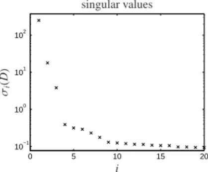
At the start of the reaction only the reactant X (rac- (ebthi)-Hf(η²-Me3SiC2SiMe3) with ebthi=1,2-ethylen- 1,1’-bis(η⁵-tetrahydroindenyl)) contributes to the absorption within the spectral range [420,800]nm. The distribution of the singular values of D (see Fig. 6) clearly indicates that only three independent chemical components can be found. In other words the perturba- tion matrix E in D =CA+E seems to be close to the zero-matrix. Therefore a truncated singular value de- composition of D ∈ R^500×381+ is to be determined with factors C∈R^500×3+ and A∈R^3×381+ .

500 600 700 800

0 0.5 1 1.5 2

wavelength [nm]

absorption

Series of spectra

Figure 5: Series of spectra in the rows of the matrix D.

0 5 10 15 20

10⁻¹ 10⁰ 10¹ 10²

i σi(D)

singular values

Figure 6: Semi-logarithmic plot of the 20 largest singular values of data matrix D.

The initial concentration of X is cX(0) = 0.01309 mol L⁻¹. Assuming that the conversion to Z at t = 2.495s is complete the last spectrum is that of the pure component Z (only traces of X and Y are present). Therefore fairly accurate spectra of the reactant X and the product Z are available, see Fig. 7.

We use the following notation and plot-line-style for the three components

C(i,1)=c_X(t_i), A(1,j)=a_X(λ_j), (line: solid), C(i,2)=cY(ti), A(2,j)=aY(λj), (line: dashed), C(i,3)=cZ(ti), A(3,j)=aZ(λj), (line: dash-dotted) with i = 1, . . . ,500 and j = 1, . . . ,381. Hence A(1,:) and A(3,:) are known parts of the factorization D=CA.

6.1. The complementary concentration profile

Two spectra of the three-component system are known. Thus Theorem 4.2 and Corollary 4.3 determine the concentration profile C(:,2) of the (unknown) in- termediate Y. This concentration profile, see Fig. 8, is uniquely determined aside from (positive) scaling.

6.2. The associated concentration profiles

The coupling theorem 4.6 can be applied to derive affine linear representations of the unknown concentra- 10

(11)

500 600 700 800 0

50 100 150

wavelength [nm]

absorption

Spectra of reactant and product

Figure 7: Spectra of rac-(ebthi)Hf(C4H8) (solid) and rac- (ebthi)Hf(η²-Me3SiC2SiMe3) (dash-dotted).

0 0.5 1 1.5 2

0 0.1 0.2 0.3 0.4 0.5 0.6

time [s]

relativeconcentration

Concentration profile.

Figure 8: Concentration profile (arbitrarily scaled) of the intermediate Y.

tion profiles C(:,1) and C(:,3) in the form C(:,1)=U ˜˜Σ(υ1+αw), C(:,3)=U ˜˜Σ(υ2+βw).

The vectorsυ1, υ2,w ∈ R³ are determined as follows (cf. Theorem 4.6 and Section 5.2)

A([1,3],:) ˜Vυ₁=(1,0)^T, A([1,3],:) ˜Vυ2=(0,1)^T, A([1,3],:) ˜Vw=(0,0)^T.

Once again the complementarity theorem 4.2 is ap- plied. It allows to conclude from the two profiles C(:,1) and C(:,3) on the remaining spectrum A(2,:) of the in- termediate. As C(:,1) and C(:,3) depend onαandβthe spectrum A(2,:) given by

A(2,:)=γ1V(:,˜ 1)+γ2V(:,˜ 2)+γ3V(:,˜ 3) (17) also depends on these constants. Therein ˜V(:,i) are right singular vectors andγi=γi(α, β) are real constants.

This results in the following two-parametric approxi-

0 1

2 0

0.1 0.2 0 0.5 1

time [s]

α

Continuum of C(:,1)[α]

0 1

2

−1

−0.5 0 0 0.5 1

time [s]

β

Continuum of C(:,3)[β]

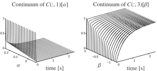
Figure 9: Continua of concentrations profiles C(:,1)[α] and C(:,3)[β].

mate factorization D≈CA with

C=(C(:,1)[α], C(:,2),C(:,3)[β]), A=







D(1,:) A(2,:)[α, β]

D(k,:)







. (18)

Therein the dependence of certain columns and rows on the parametersαandβis expressed by rectangular brackets.

6.3. Non-negativity constraints

Only a componentwise non-negative concentration factor C makes sense. For the vectors υ1, υ2,w ∈ R³ and ˜V(:,i) ∈ Rⁿ (which are known from Section 6.2) onlyα∈ [−0.078,0.245] andβ ∈ [−1.186,0.0278] re- sult in a non-negative matrix C, cf. Theorem 4.7. The resulting continua for the concentration profiles C(:,1) and C(:,3) are shown in Fig. 9.

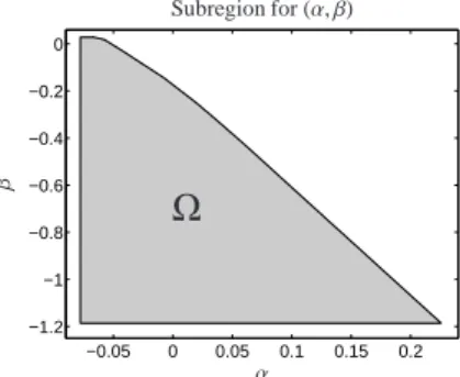
The Cartesian product interval (α, β) ∈ [−0.078,0.245] × [−1.186,0.0278] can fur- ther be restricted as A(2,:) also depends on α and β, see Equation (17). The subregion of [−0.078,0.245] × [−1.186,0.0278] which guaran- tees non-negative spectra A(2,:)[α, β] is shown in Fig. 10. This subregion of admissible parameters is denoted byΩ. These further restrictions are derived in a way which is comparable to (FIRPOL in) the Borgen approach [4].

6.4. Best fit with a kinetic model

Up to now the rotational ambiguity of the solu- tion matrices C and A has considerably been reduced and the remaining ambiguity, see Eq. (18), has been parametrized in the parametersαandβ. The concentra- tion profile of the intermediate Y has been determined uniquely. Further the concentration profiles of the reactant and the product one-parameter representations have been derived. The spectrum A(2,:) has a two-parameter form.

11

(12)

−0.05 0 0.05 0.1 0.15 0.2

−1.2

−1

−0.8

−0.6

−0.4

−0.2 0

α

β

Ω

Subregion for (α, β)

Figure 10: RegionΩof pairs (α, β) which guarantee non-negative con- centration profiles C(:,1)[α], C(:,3)[β] and a non-negative spectrum A(2,:)[α, β].

The next step is to find in the region of parameter- pairs (α, β), see Fig. 10, those solutions which are consistent with a kinetic model

X−→^k¹ Y −→^k² Z. (19) The computational procedure is as follows: For the pairs (α, β) ∈ Ω the factors (18) are computed. Then the concentration factor C[α, β] is fitted to the kinetic model associated with (19) and k₁and k₂are determined simultaneously. This is a hard-model-fit for each admissible pair (α, β). We are interested in determining those (α, β) ∈ Ω which are responsible for the best possible fit. The concentration profiles in C∈R^500×3are scaled in a way that the sumP3

i=1C(:,i) equals the initial con- centration cX(0) at any time (due to the mass balance).

Then a nonlinear regression is used to compute the ki- netic constants k1and k2in a way that the kinetic equations for (19) fit the concentration profiles.

The optimal kinetic constants k^∗₁, k^∗₂and optimal pa- rametersα^∗andβ^∗minimize the functional

G :R²+×Ω→R, (k₁,k₂, α, β)7→

X3

i=1

X500

j=1

γ⁻²_i

(Cji(α, β)−C^(ode)_ji (k1,k2))2

. (20)

The matrix C^(ode) ∈ R^500×3contains (the values on the time×wavelength grid of) the solution of the initial value problem

dcX(t)

dt =−k1cX(t), cX(0)=0.01309, dcY(t)

dt =k1cX(t)−k2cY(t), cY(0)=0, dcZ(t)

dt =k2cY(t), cZ(0)=0.

0 0.1 0.2

−1

−0.5 0

α

β

Contour lines of ¯G

0 0.1 0.2

−1

−0.5 0 10⁰ 10¹

β α

¯ G(α,β)

3D plot of ¯G

Figure 11: Error by fitting the kinetic model on the decomposition depending on (α, β), error plot and contour lines.

Its analytic solution reads

C^(ode)(t; k1,k2)=







c_X(0) exp(−k₁t)

c_X(0)k₁

k₂−k₁ (exp(−k₁t)−exp(−k₂t)) cX(0)(1+^k²^exp(−k¹_k^t)−k¹^exp(−k²^t)

1−k₂ )





 .

Additionally scaling factors γi= max

l=1,...,500Cli, i=1,2,3,

are used in Equation (20) for a proper relative weighting of the errors for the three species X, Y and Z.

As k1 and k2 depend on α and βthe minimization problem reads

G :¯ Ω→R, (α, β)7→ min

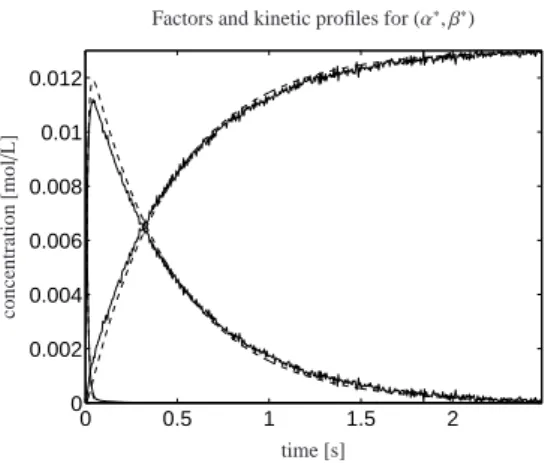
k1,k2∈R⁺G(k1,k2, α, β). (21) The contour lines of ¯G together with a 3D plot are shown in Fig. 11. The numerical minimization results inα^∗ =−0.078 andβ^∗ =−1.186. The associated opti- mal kinetic constants are k^∗₁ =93.99s⁻¹(instable result due to the poor ratio of the injection phase (5ms) and the reaction phase (45ms) with spectra taken every 5ms) and k₂^∗=2.152s⁻¹. The concentration profiles of the re- actant X, of the intermediate Y and of the product Z are shown in Fig. 12. The solutions C^(ode)(t; k^∗₁,k^∗₂) are con- sistent with the concentration profiles C(:,i), i=1,2,3.

The remaining small errors at t ≈ 0 are caused by the computational procedure which for all quantities guar- antees non-negativity – a regularized SMCR approach as in [15, 22] can produce nearly accurate approximations.

6.5. Critical remark

The results which have been derived in this section can also be extracted by using conventional approaches:

First chemometric tools allow to recover the kinetic constants from the spectroscopic data together with the knowledge of the kinetic model. This allows to construct the concentration profiles and then to compute 12