Comparative multivariate curve resolution study in the area of feasible solutions

(1)

Comparative multivariate curve resolution study in the area of feasible solutions

Henning Schröderâ,b, Mathias Sawallâ, Christoph Kubis^b, Annekathrin Jürßâ, Detlef Selent^b, Alexander Brächer^c, Armin Börner^b, Robert Franke^c,d, Klaus Neymeyrâ,b

aUniversit¨at Rostock, Institut f¨ur Mathematik, Ulmenstrasse 69, 18057 Rostock, Germany

bLeibniz-Institut f¨ur Katalyse, Albert-Einstein-Strasse 29a, 18059 Rostock, Germany

cEvonik Performance Materials GmbH, Paul-Baumann Strasse 1, 45772 Marl, Germany

dLehrstuhl f¨ur Theoretische Chemie, Ruhr-Universit¨at Bochum, 44780 Bochum, Germany

Abstract

Multivariate curve resolution (MCR) methods as MCR-ALS, ReactLab, the peak group analysis and SVD-based hard- modeling methods differ in their algorithms and the underlying optimization procedures. These differences include variants in the implementation of the algorithms and a differing weighting of the constraints. Depending on the MCR method different computational results can be obtained for the same data set.

The area of feasible solutions (AFS) comprises all possible outcomes of MCR methods. It represents all nonnegative factors of a given spectral data set. It therefore offers an unbiased view of the problem. In a comparative study we present within the AFS the various MCR results for a model data set and for experimental FTIR data. For the model data we observe that the spread of the MCR results correlates with the so-called purity of the spectral data.

Key words: Multivariate Curve Resolution, Nonnegative Matrix Factorization, Area of Feasible Solutions, MCR-ALS, ReactLab, FACPACK,

1. Introduction

Multivariate curve resolution (MCR) and self- modeling curve resolution (SMCR) techniques serve to extract the underlying pure component information from spectroscopic mixture data. For example, these data can be taken from spectral observation of an on- going chemical reaction. If a number of n spectra is recorded over the reaction time and if each spectrum contains m spectral channels, then the spectral measure- ment can be stored in an n-by-m data matrix D. Its ith row contains the ith mixture spectrum.

The MCR problem is to determine the number s of chemical components, their pure component spectra together with the associated concentration profiles.

The basis for the solution of the MCR problem is the Lambert-Beer law in matrix form

D=CA. (1)

It expresses a bilinear relation between D and the matrix of pure component spectra A∈ R^s^×^mtogether with the matrix C∈Rⁿ^×^sof the associated concentration profiles of the s pure components. In the case of noisy data or af- ter approximate baseline subtraction the Lambert-Beer

law is assumed to hold at least approximately. The pure component recovery problem amounts to determining the nonnegative matrix factors C and A for the given matrix D of spectral data. The key-problem with the factorization (1) is the so-called rotational ambiguity of the solution [1, 2, 3]. This means that often continua of nonnegative matrices C and A exist so that D=CA.

The so-called area of feasible solutions (AFS) is a low- dimensional representation of the set of all these nonnegative matrix factors [4, 5, 6, 7]. In contrast to this, MCR techniques aim at determining a single, namely the chemical meaningful and hopefully correct solution.

This paper presents and compares the results of some frequently used MCR program codes within the AFS setting. This includes variations in the constraint selection and a varying weighting of the constraints. We use the MCR software packages MCR-ALS [8, 9], Re- actLab [10] and the Peak group analysis (PGA) [11], which is a part of the FACPACK software [12]. We also consider a hard-modeling approach [13, 14]. Further, the AFS is computed and the various MCR results are graphically highlighted within the AFS. This demon- strates not only that the AFS comprises all possible non-

(2)

negative factorizations of D, but also illustrates the pos- sible variations of the program output of MCR methods as a consequence of the underlying rotational ambiguity. The “MCR-in-AFS” representation is considered for model data and also for an experimental FTIR spectral data set. Further, we analyze the relation of the closeness of measured spectra to the AFS and the spread of the various MCR results within the AFS. We hope that our study can improve the awareness on the reliability of MCR methods, on the impact of a proper parametrization and constraint selection of MCR methods and, last but not least, on the important influence of kinetic hard modeling, which can considerably reduce the rotational ambiguity.

1.1. Organization of the paper

Section 2 contains a brief introduction to the nonnegative matrix factorization problem and an overview about some widely used MCR software packages. A short introduction to the AFS is given in Section 3. Sec- tion 4 proposes two data sets and presents the computational results for the various MCR codes. The purity of spectral mixture data is investigated in the context of the spread of various MCR results.

2. Pure component recovery

MCR algorithms aim at extracting chemically interpretable and in the best case correct pure component factors C and A so that D=CA reconstructs the spectral data matrix D. To this end an MCR algorithm can solve a minimization problem for a target function

f (C,A)= kD−CAk²F

| {z } reconstruction error

+ kmin(C,0)k²F

| {z }

C≥0

+kmin(A,0)k²F

| {z }

A≥0

+ g(C,A)

| {z }

constraints

. (2)

Therein,k · k^F denotes the Frobenius norm (square root of the sum of squares). The minimization of f (C,A) by (2) with respect to C and A should result in a small reconstruction error and should result in only few and small negative entries in C and A. A weighted sum of constraints

g(C,A)=ω1fkin(C,A) +ω2funi(C,A) + ω3fmono(C,A) + . . .

with positive weight constantsω_ican be used in order to favor specific properties of the solution. The additional constraints allow us to favor the consistency of

the concentration profiles C with a kinetic model, to support unimodular or monotone concentration profiles or to find spectra with certain properties (either sharp localized peaks or smooth spectra) and so on. See for example [1, 15, 8, 16, 17] and the references therein.

A main effect of these constraints is that they can reduce the rotational ambiguity. The term “rotational ambiguity” refers to the fact that from a given matrix fac- torization D=CA with nonnegative factors C and A of- ten many differing nonnegative factorizations D =CeAe can be constructed by means of a regular matrix T ac- cording to

D=CA=(CT⁻¹)

| {z }

e C≥0

(T A)

|{z}

e A≥0

. (3)

These new nonnegative factorsC ande A still reconstructe D. Typically, continua of possible nonnegative factor- izations of D exist. The trivial scaling ambiguity, which represents the fact that the factorization (3) may also include the factors∆⁻¹∆with a nonnegative regular di- agonal matrix∆can be neglected as all algorithms, see Sec. 2.1, make use of a certain fixed scaling. Compu- tationally, C and A are in many cases constructed from the bases of left and right singular vectors of D [18, 17].

This requires a low-rank approximation of D by the sin- gular value decomposition [19].

2.1. MCR software packages

For our AFS analysis of MCR results we select the following MCR software packages from the wide port- folio of available software solutions:

• MCR-ALS The Multivariate Curve Resolution Alternating Least Squares (MCR-ALS) code, see

http://www.mcrals.info

is the most prominent and potentially most often used MCR software. It is available in the form of a MatLab toolbox. MCR-ALS uses an SVD- free minimization procedure which applies the constraints to the approximate factors C and A within an iterative ALS optimization, see [8, 9].

MCR-ALS includes various constraints, e.g., those on nonnegativity, unimodality, equality, closure and on the consistency with a kinetic model.

MCR-ALS additionally allows the analysis of multi-way data.

• ReactLab The ReactLab software tools http://jplusconsulting.com

for revealing chemical reaction mechanisms, see [10], combines Excel sheets for the data import 2

(3)

with an MatLab graphical user interface to the computational core routines. In ReactLab the underlying ssq-based minimization uses an adapted Levenberg-Marquardt algorithm and the kinetic equations are numerically solved by a fourth order Runge-Kutta method. Further, the linearly independent components are identified in a model-free analysis which uses a singular value decomposition of the spectral data matrix.

• The kinetic SVD-based hard-modeling approach is described in [14]. This approach minimizes a con- straint function g which measures the consistency of the spectral data with a given kinetic model.

The model fit by means of a numerical optimization procedure includes the computation of optimal reaction rate constants. The predicted con- centration profiles C and the associated spectra A minimize the reconstruction error D−CA. This hard-modeling approach with integrated rate constants optimization is very strong in reducing the rotational ambiguity.

• The peak group analysis (PGA), see [11], is a win- dowed MCR approach which constructs step-by- step a pure component decomposition. PGA starts with a user-selected frequency window of the spectral data set and tries to detect peak correlations from the selected window to the remaining spectra outside the window. In this respect PGA is similar to the window factor analysis (WFA) [20]. PGA allows the user to select problem adapted constraints and the associated weight factors. The software is an explorative analysis method for spectral data which contains many unknown quantities. It requires a steering of the decomposition process by an experienced chemist who can find and iden- tify possible pure components. PGA is a part of the FACPACK toolbox, see http://www.math.uni- rostock.de/facpack [12].

3. Area of feasible solutions

A global approach to solving the MCR problem is to determine the set of all possible factorizations D = CA with nonnegative matrix factors C and A. This set of feasible factorizations can be represented in a low-dimensional way by the Area of Feasible Solutions (AFS), see e.g. [4, 5, 21, 22, 23, 6, 24, 25, 26]. The AFS for a chemical s-component system is a bounded subset of (s−1)-dimensional space. A point in the AFS is a vector of expansion coefficients with respect to either the left singular vectors (concentration profiles) or

right singular vectors (spectra) of the spectral data ma- trix D. In this sense the AFS represents the continua of all possible spectra and of all possible concentration profiles. Most of the solutions cannot be interpreted chemically and are called abstract factors. The top row of Fig. 3 shows the concentrational AFS and the spectral AFS for a three-component system; the underlying three-component model problem is introduced later in Section 4.1. The colored markers in the AFS sets represent certain spectra or concentration profiles which are also plotted in the remaining rows of Fig. 3.

The AFS provides an unbiased overview of all feasible factorizations. AFS computations can be combined with additional constraints [27, 28, 29, 30, 31]. An AFS computation under additional constraints emulates an MCR technique. However, the AFS-based approach has the advantage that it always allows a full control of the solution selection procedure. AFS computations can be done by the FACPACK software [32, 12] which combines a MatLabgraphical user interface (GUI) with core programs written in C and Fortran. FACPACK with the default parameter settings has been used for all AFS computations in this paper.

4. An MCR-in-AFS analysis

This section contains a short comparative study of MCR results and their AFS representations. First Sec- tion 4.1 introduces a model data set and an experimental FTIR data set. In Section 4.2 the four MCR algorithms from Section 2.1 are applied to these data sets. Addi- tionally, the associated AFS sets are computed. Then the MCR results are marked within the AFS. In order to represent the MCR-ALS results in the AFS (MCR- ALS does not use an SVD of D), the computed spec- tra and concentration profiles are expanded with respect to the bases of either right or left singular vectors [3, 33, 34, 35]. The resulting expansion coefficients are the basis for the AFS representation. The presen- tation of the MCR results is accompanied by a critical discussion. Finally, Section 4.3 investigates the relation of data purity and the spread of the MCR results in the AFS.

4.1. Data sets

We consider the following three-component (sub)systems:

1. Model data:

The reaction scheme

X k₁ GGGGGB F GGGGG

k₋1

Y k2

GGGA Z (4)

3

(4)

with the rate constants k1=4, k₋1=1 and k2=2 and initial concentrations of (X,Y,Z) at t = 0 are (1,0,0). Then numerical integration of the kinetic equations yields the concentration profiles. The pure component spectra of X, Y and Z are taken as Gaussian profiles with a moderate overlap. The concentration profiles and the spectra are shown in Fig. 1. The model is discretized by taking n=101 equidistant time-points in [0,3] and a number of m=201 spectral channels. Thus D is a 101×201 matrix.

2. Rhodium catalyzed hydroformylation:

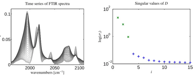
The experimental FTIR data set includes n=1353 spectra, each with m = 610 data channels. The s=3 main absorbing components in the frequency window [1960,2120]cm⁻¹ are the olefin component, a hydrido complex and an acyl complex. See [36] for the chemical details on this homogeneous catalytic reaction (sub)system; here we used the p(H₂)=1.01MPa data set from [36]. The reaction complies with the Michaelis-Menten kinetic model

S +K k₁ GGGGGB F GGGGG

k₋1

S K k2

GGGA P+K, (5)

which is the central ingredient for a kinetic hard- modeling approach. The absorption of the product component, namely the aldehyde, can be ig- nored in the given frequency window. The data is shown in Fig. 2. The spectral data were taken by a Bruker Tensor 27 FTIR spectrometer with a MCT-A (mercury-cadmium-telluride) IR detector.

Further details on the experimental setup are described in [36].

4.2. Comparative MCR-in-AFS analysis

This section reports on the application of the MCR variants to the two spectral data sets. Necessary con- straints are D−CA≈0 and C,A≥0. A kinetic regularization has been used in the ReactLab package and the SVD-based hard-modeling approach. MCR-ALS has been applied with and without kinetic modeling.

4.2.1. Model data

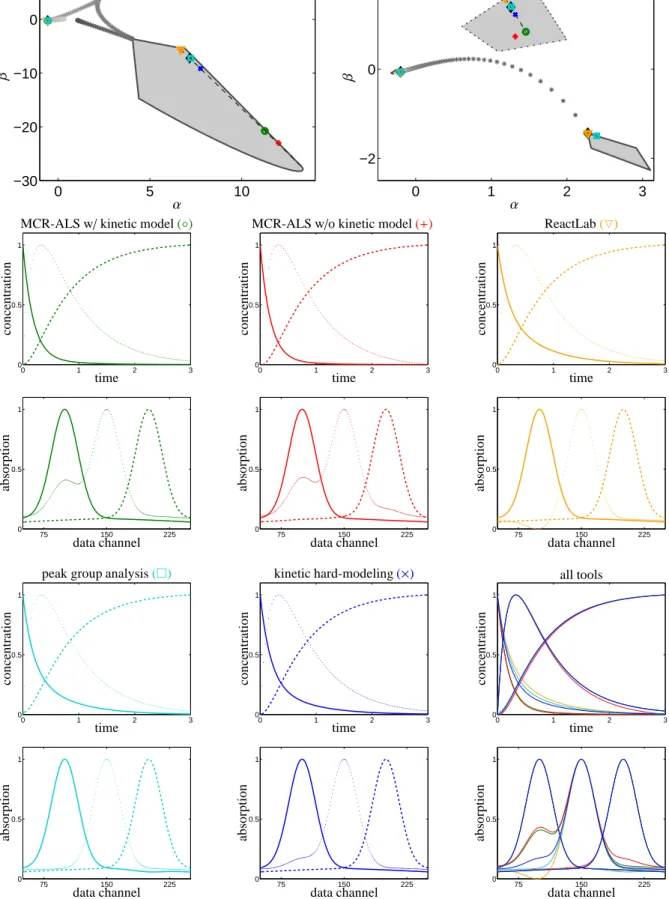
All MCR and AFS results for the model data are pre- sented in Fig. 3. The top row shows the AFS for the factor C and also the AFS for the factor A. If we take a point in the concentrational AFS with the coordinates (α, β), then the vector of expansion coefficients (1, α, β) with respect to the three dominant left singular vectors

of D allows us to compute a feasible concentration pro- file. Correspondingly, a vector (1, α, β) of expansion coefficients with respect to the three dominant right singular vectors yields a feasible spectrum. In these two AFS sets the MCR results are marked by colored sym- bols. Especially for the largest AFS segments (we call the isolated subsets of the AFS segments) these markers show a wide dispersion. The line style (solid, dashed or dotted) of the boundary of an AFS segment has been used again for the same chemical components in the remaining plots of Fig. 3 in its rows 2 up to 5 in order to represent the associated concentration profiles and spectra. These plots show the results of MCR-ALS with and without kinetic regularization, of ReactLab, of PGA and of SVD-based kinetic modeling. The five different line colors of the markers in the AFS plots indicate which one of the MCR methods has been used (green for MCR-ALS with kinetic modeling, red for MCR- ALS without kinetic modeling and so on). The rows of D are represented in the spectral AFS by stars chang- ing from dark black to gray in the course of the reaction.

Correspondingly, the columns of D are represented by stars in the concentrational AFS.

For this first-order reaction system X ⇋ Y → Z the analysis in [14] shows that even with the inclusion of a kinetic model with optimally adapted reaction rate constants, see Table 1, no unique nonnegative factoriza- tion D=CA can be found. This result is confirmed by the various MCR results. The two AFS plots in Fig. 3 show black dotted lines in each of the largest AFS subsets. All points on these lines belong to solutions which are consistent with an optimally parametrization of the given kinetic model, see [14]. In fact, we observe that the MCR results of all methods which use a kinetic regularization are located on these lines. Not surprisingly the MCR-ALS result without kinetic modeling (marked by a red+symbol) is not located on this line in the spectral AFS.

Remark 4.1. For a given reaction scheme, e.g. by Eq. (4), and for given reaction rate constants the con- centration profiles of all chemical components can be computed if the initial concentrations are known. For an s-component system and if a discrete time grid with n points is considered, then these discrete concentration profiles can be stored in the columns of an n-by-s matrix Côde. We call such a vector of reaction rate constants D-consistent if the resulting matrix Côde is a possible factor in a nonnegative matrix factorization D=CôdeA of the given spectral data matrix D, see [14] for the de- tails.

In [14] the set of all D-consistent reaction rate con- 4

(5)

75 150 225 0

0.5 1

data channel

absorption

Spectral mixture data D

0 1 2 3

0 0.5 1

concentration

time Concentration profiles

75 150 225

0 0.5 1

data channel

absorption

Pure component spectra

Figure 1: The model data set: The left subplot shows each fourth row of the spectral data matrix D. The line color starts with a dark black and ends in gray in the course of the reaction. The centered plot shows the concentration profiles according to X↔ Y→ Z. The pure component spectra are shown on the right. The color assignment is X blue, Y green, Z red.

2000 2050 2100

0 0.05 0.1

wavenumbers [cm⁻¹]

absorption

Time series of FTIR spectra

0 5 10 15

10⁻² 10⁰ 10²

Singular values of D

i log(σi)

Figure 2: Experimental FTIR data set on the rhodium catalyzed hydroformylation process: The left subplot shows each 30th row of the data matrix.

The line color starts with a dark black and ends in gray in the course of the reaction. The first 15 singular values of the spectral data matrix D are plotted on the right. The three largest singular values (x) are clearly separated from the remaining smaller ones (+). This clearly indicates a (noisy) three-component system.

Computed reaction rate constants and relative reconstruction errors

Model data set Experimental FTIR data

MCR software k₁ k₋₁ k₂ err_D err_k k₁ k₋₁ k₂ err_D err_k

MCR-ALS 5.31 0.18 1.51 2.9·10⁻⁷ 1.2·10⁻⁶ 77.18 6.46 4.66 2·10⁻² 8.3·10⁻⁵ ReactLab 3.60 1.18 2.22 1.6·10⁻⁵ 3.5·10⁻³ 370.7 34.42 4.28 6·10⁻³ 1·10⁻² hard-modeling 4.34 0.82 1.85 1.8·10⁻¹⁵ 1.8·10⁻¹⁰ 32.08 10⁻⁹ 4.63 4·10⁻³ 8.8·10⁻⁵

Table 1: The table lists the reaction rate constants as computed by the kinetic-model-based MCR tools as introduced in Sec. 2.1. Two data sets are considered, see Sec. 4.1. For each of these data sets the computed rate constants show major differences whose cause is explained in the remarks 4.1 and 4.2. Small (relative) reconstruction errors errD =kD−CAkF/kDkF indicate that the MCR codes have produced correct factorizations D≈CA. Additionally, small errors of the kinetic fit errk=kC−C^odekF/kCkF(the matrix C^odecontains in its columns the numerical solution of the kinetic equations for the given parametrization k) confirm the correctness of the reaction rate constants. These data show that even kinetic hard modeling cannot always produce unique MCR results (if the chemical reaction contains reversible steps).

5

(6)

0 5 10

−30

−20

−10 0

α

β

0 1 2 3

−2 0 2

α

β

0 1 2 3

0 0.5 1

concentration

time

MCR-ALS w/kinetic model(◦)

0 1 2 3

0 0.5 1

concentration

time

MCR-ALS w/o kinetic model(+)

0 1 2 3

0 0.5 1

concentration

time ReactLab(▽)

75 150 225

0 0.5 1

data channel

absorption

75 150 225

0 0.5 1

data channel

absorption

75 150 225

0 0.5 1

data channel

absorption

0 1 2 3

0 0.5 1

concentration

time

peak group analysis()

0 1 2 3

0 0.5 1

concentration

time

kinetic hard-modeling(×)

0 1 2 3

0 0.5 1

concentration

time all tools

75 150 225

0 0.5 1

data channel

absorption

75 150 225

0 0.5 1

data channel

absorption

75 150 225

0 0.5 1

data channel

absorption

Figure 3: Results of the MCR-in-ALS analysis for the model data set. Top row: AFS for the factor C and the AFS for the factor A. A triple of expansion coefficients (1, α, β) with respect to the left singular vectors represents a concentration profile and with respect to the right singular vectors a spectrum is represented. In these two AFS sets the MCR results are tagged by colored markers. The rows of D are represented in the spectral AFS by stars changing from dark black to gray in the course of the reaction. Correspondingly, the columns of D are represented by stars in the concentrational AFS.

Second to fifth row: The colored markers in the AFS for the various MCR methods correspond to specific concentration profiles and spectra.

These are shown in the same line color for MCR-ALS with and without kinetic regularization, for ReactLab, for PGA and for SVD-based kinetic modeling. The line style (solid, dashed, pointed) corresponds to the line style of the boundary curve of the associated AFS subset. Bold dashed lines are used to mark in the two AFS sets those solutions which are consistent with a kinetic model for optimally adapted rate constants, see [14]

for the theoretical background. In the spectral AFS this black dashed line is mostly covered by result markers.

The last two plots show all MCR results in overlaid form which indicates that the MCR codes have produced to some extent qualitatively different results.

6

(7)

stantsKfor the model reaction (4) has been determined analytically as follows

K =







 α β(α) γ(α)



: α∈

"ψ− √ φ 2 ,ψ+√

φ 2

#



with

ψ=k^∗₁+k^∗₋₁+k^∗₂, φ=(k₁^∗+k^∗₋₁+k₂^∗)²−4k^∗₁k₂^∗, β(α)=−1

4

(ψ−2α)²−φ

α , γ(α)=ψ−α−β(α).

and the given k^∗ = (4,1,2)^T for the model data set.

The strongly varying values of k1, k₋1 and k2 for the model data set in Table 1 reflect the fact that even an underlying kinetic model cannot result in unique re- action rate constants. The correctness of these rela- tions is confirmed by small reconstruction errors err_D= kD−CAk^F/kDk^F and by small errors of the kinetic fit errk = kC−C^odek^F/kCk^F. See [14] for all analytical details.

The last two plots in Fig. 3 (all lines are plotted black) show all MCR results in overlaid form. To some extent we observe qualitatively different results especially for the computed spectra of the intermediate Y. More- over, the concentration profiles of the reactant X show a somewhat different decay behavior.

For this model problem the analysis underlines the advantage of the global AFS approach. All possible nonnegative factorizations are easily accessible. The user can locate the MCR results in the AFS and he can decide whether or not a certain spectrum or concentration profile is chemically meaningful. For this model problem the peak shape of the component Y exhibits a considerable variation, which might help the chemist to steer the factorization process in the desired and chemically interpretable direction.

The MCR experiments for this data set show that even MCR methods without kinetic regularization work surprisingly well. In principle, an MCR method which only requires that C,A≥0 and D≈CA can produce any so- lution which is represented in the AFS. However, these methods in some cases tend to yield pure components which are close to the purest components in the measured data, see also the discussion in Section 4.3 on data purity. For instance, MCR-ALS allows to initialize the iterative alternating least squares procedure by the “pure variables” of either A or C. Then it is plausible that the iteration terminates in a close neighborhood.

4.2.2. Rhodium catalyzed hydroformylation

For this noisy FTIR data set we first compute the sin- gular values of D, see Fig. 2. The three largest singu-

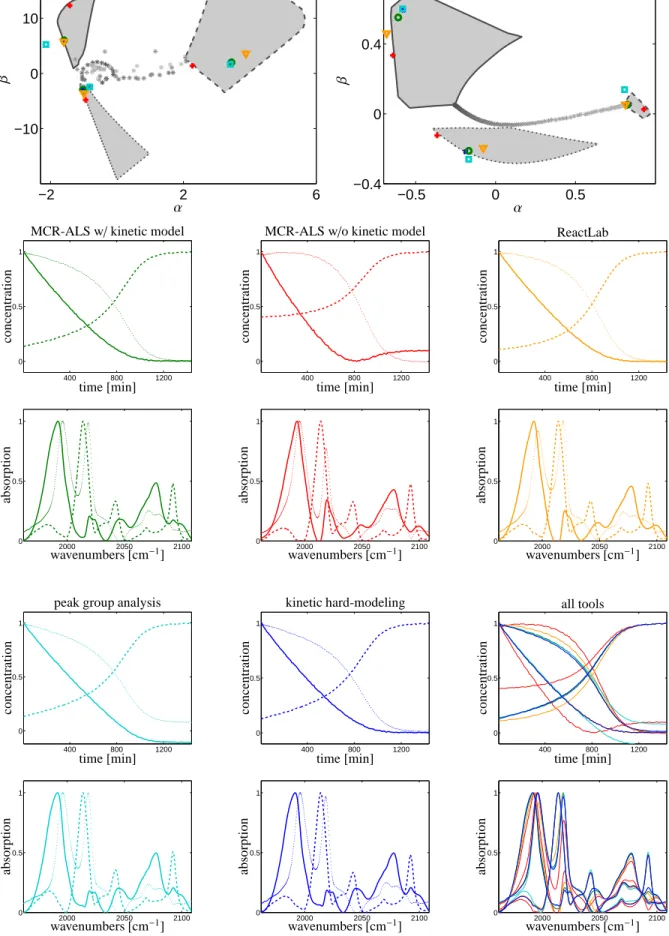
lar values are characteristically larger than the remaining singular values. This indicates a three-component system and justifies to work with a rank-3 approxima- tion of D in the SVD-based MCR algorithms. Figure 4 shows all MCR- and AFS-computational results. The meaning of the line-styles, markers and marker colors is explained in Sec. 4.2.1 and the caption of Fig. 3.

MCR-ALS with kinetic modeling, ReactLab and SVD-based kinetic hard modeling all include the consistency with an optimally parametrized Michaelis- Menten model. However, the computed reaction rate constants in Table 1 show strong variations as the Michaelis-Menten model due to its reversible subreac- tion does not allow to determine unique rate constants, see Remark 4.2. The concentration profiles, spectra and boundaries of the respective AFS segments are drawn by solid lines for the olefin, by dashed lines for the hydrido complex and by dotted lines for the acyl complex, see also [36]. For these three MCR methods with kinetic modeling small deviations can be seen in the concentration profiles of the hydrido complex and the acyl complex as well as in the spectra of olefin and the acyl complex. The resulting factorizations are chemically interpretable which is a result of the strong regularization of the underlying Michaelis-Menten model.

MCR-ALS without kinetic regularization results in an almost feasible factorization with some small negative entries. The associated AFS representations of the factors (red+markers) are partially located outside the AFS segments. A further approximation is needed for the graphical representation of the MCR-ALS results in the AFS: Since MCR-ALS is an SVD-free method we need for the AFS representation of the MCR-ALS results a projection to the spaces of the three dominant left (respectively right) singular vectors. We also observe in Fig. 4 that the concentration profile of the olefin is not a monotone function with a minimum at about t = 800min. Such a non-monotone function is an abstract factor without useful chemical interpretation.

The PGA focuses on the reconstruction of the spectral profiles. The optimal results from [36] can be re- produced very well. Then the concentration profiles are calculated after the complete determination of the factor A. This results in small negative entries in the concen- tration profile of the olefin component.

Once again, this experimental data set documents the usefulness of the AFS approach. Chemically interpretable pure components can easily be extracted from the AFS. The user is not limited to a certain MCR solution but can explore the set of all other feasible factorizations.

7

(8)

−2 2 6

−10 0 10

α

β

−0.5 0 0.5

−0.4 0 0.4

α

β

400 800 1200

0 0.5 1

concentration

time [min]

MCR-ALS w/kinetic model

400 800 1200

0 0.5 1

concentration

time [min]

MCR-ALS w/o kinetic model

400 800 1200

0 0.5 1

concentration

time [min]

ReactLab

2000 2050 2100

0 0.5 1

absorption

2000 2050 2100

0 0.5 1

absorption

2000 2050 2100

0 0.5 1

absorption

400 800 1200

0 0.5 1

concentration

time [min]

peak group analysis

400 800 1200

0 0.5 1

concentration

time [min]

kinetic hard-modeling

400 800 1200

0 0.5 1

concentration

time [min]

all tools

2000 2050 2100

0 0.5 1

absorption

2000 2050 2100

0 0.5 1

absorption

2000 2050 2100

0 0.5 1

absorption

Figure 4: Results of the MCR-in-ALS analysis for the rhodium catalyzed hydroformylation data set: See the caption of Figure 3 for an explanation of the subplots, the color assignment the meaning of the different line styles and the data representation by the black to gray stars in the AFS plots.

The colored markers in the AFS sets, which represent the different MCR results, are somewhat more scattered in the AFS sets. Partially, they are even outside the AFS which indicates that the nonnegativity constraint is violated. The right lower two plots, which show all MCR results in overlaid form, indicate a much stronger variation of the MCR results for this experimental FTIR data set.

8

(9)

11 30 60 90 0

0.5 1

Spectral data purity

row index of D

distancetonearestAFSsegment

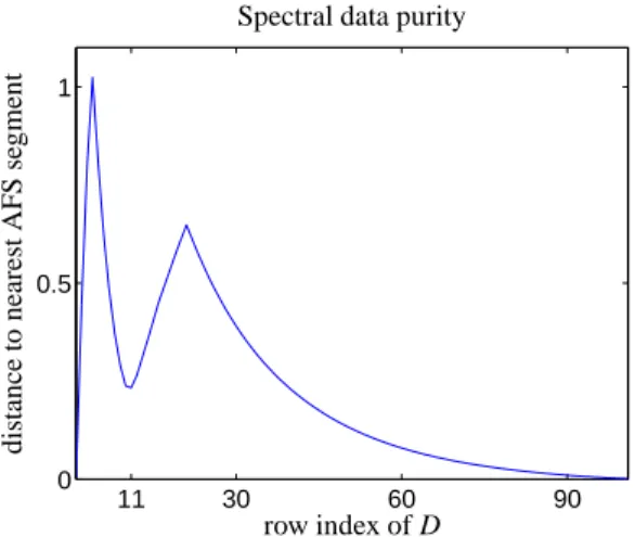
Figure 5: Plot of the Euclidean distances of the row representations of D to the closest points in the AFS for the model data set. This is a measure for the closeness of a measured spectrum to a possible pure component spectrum. We call this data purity. The curve has three local minima, namely in the first, 11th and last spectrum. This corresponds to maximal concentrations of the reactant, intermediate and reaction product.

Remark 4.2.

I Analogously to the situation as explained in Re- mark 4.1, the Michaelis-Menten kinetic model is not sufficient to guarantee a unique MCR factor- ization if the ratio S0/K0 of initial concentrations is large. If a certain optimally adapted vector k^∗of kinetic constants is known, then the set of all these vectors of rate constantsKcan be computed. The reaction rate constant k^∗₂is unique (aside from per- turbations) and k1and k₋1satisfy the relation

k₋₁=K_mk₁−k^∗₂ with K_m= k^∗₋₁+k^∗₂ k^∗₁ .

II For our computational experiments we had to sub- stitute the MatLab ordinary differential equation (ode) solver “ode45” in the MCR-ALS code by the stiff ode solver “ode15s”. This has reduced the computation from about three hours to less than a minute. Additionally, we had to thin out the matrix D for the ReactLab MCR code as the dimensions of the data sets exceed the limitations of the Excel software, which is used for data import in React- Lab.

4.3. Data purity and spread of MCR results

In this section we investigate the relation of data pu- rity and the spread of the MCR results in the AFS rep- resentation. (Euclidean distances in the spectral AFS

Spread in AFS segment solid dotted dashed All MCR methods 0.041 0.309 0.0046 Only MCR w/kin. mod. 10⁻⁷ 0.26 10⁻⁵

Table 2: Spread of MCR results by Eq. (6) in the AFS segments, see Sec. 4.2.1.

MCR spread in AFS segments

Noise solid dotted dashed

Heteroscedastic 2% 0.257 0.475 0.007 Homoscedastic 2% 0.086 0.403 0.025 Heteroscedastic 5% 0.462 0.534 0.029 Homoscedastic 5% 0.260 0.480 0.022

Table 3: Homoscedastic and heteroscedastic noise with signal-to- noise ratios of 2% and 5% is added to the model data set. The resulting spread, see Eq, (6), of the MCR results in the AFS representation is listed.

are equal to the Euclidean distances of the associated spectra; see the remark after Eq. (6).) Under data purity we understand how close a measured spectrum (taken from the chemical reaction system) is to the possible pure component spectra. In other words a spectrum is called pure, if only one chemical component contributes to the absorption. Typically, spectra are nearly pure at the beginning of a chemical reaction if only the reactant is present and at the end of a complete chemical reaction, see also [3]. For the following analysis we use only the model data set as introduced in Sec. 4.2. Our hypothesis is that a high data purity makes it easy for MCR algorithms to extract the pure components. This would result in a small variation or spread of the MCR results in their AFS representation.

We start with the data purity analysis in the spectral AFS as shown in the right subplot of the top row in Fig.

3. The series of gray stars represent the rows of the spectral data matrix. The spectral data start at the right AFS segment with the solid boundary line which repre- sents the possible spectra of the reactant X. The series of data representing stars tends to the small left AFS segments which represent the more or less unique spectrum of the product Z. The Euclidean distances to the nearest AFS points are plotted in Fig. 5 against the row index of D. The curve has three local minima, namely in the first spectrum (approximately the spectrum of the reac- tant X), the 11th row of D, which is close to the possible spectra of the intermediate Y, and last spectrum. As the reaction is nearly complete the last spectrum is a good approximation of the product Z. Minima of the distance curve represent spectra which are close to pure spectra.

The distances of the first and last row of D to the closest 9

(10)

AFS points are each less than 0.004. The distance of the 11th row of D AFS segment representing possible spec- tra of Y is about 0.23, that is a relatively low purity of the measured spectra with respect to the chemical com- ponent Y.

Next, the data purity is related with the spread of the MCR results in their AFS representations. In order to form a measure for this spread we compute the sum of absolute differences

Xn i=1

kr−rik² (6) with ribeing the AFS representation of an MCR result and r being the geometric center (arithmetic mean) of all ri. The index i runs over all MCR methods. We remark that Euclidean distances in the spectral AFS are equal to distances of the associated spectra due to the or- thogonal invariance of the Euclidean norm [19]. In the case of the concentrational AFS the additional matrix of singular values destroys this invariance. Other norms can also be used [21], but then no invariance properties hold. The numerical distance values are listed in Table 2. The first row is the spread of the results for all MCR methods. This spread is considerably larger compared to the spread if only kinetically regularized MCR methods are considered. This experiment shows that the high spectral data purity of the chemical components X and Z leads to low variations of the MCR results. We remark that the observed relations seem to hold under special conditions, e.g., for consecutive reaction systems.

Next we study the effect of noise on the data purity and the spread of MCR results in the AFS. Het- eroscedastic (Nhe) and homoscedastic (Nho) uniformly distributed noise with signal-to-noise ratios (SNR) of 0.02 and 0.05 is added to the model data set, see Sec. 4.1. In MatLab we have generated in the het- eroscedastic and homoscedastic noise with the SNR r as follows:

N he=r∗ab s (D) .∗2 .∗( rand ( s i z e (D) )−0 . 5 ) N ho=r∗max ( max (D) )∗2 .∗( rand ( s i z e (D) )−0 . 5 )

The spread data in Table 3 confirms that a high data purity is still responsible for reliable and consistent MCR results. As expected, this effect vanishes more and more with a rising noise level.

5. Conclusion

MCR methods are important tools for the pure component recovery in analytical chemistry, but they suf- fer from the rotational ambiguity. Hence different MCR methods produce (often slightly) different results. These

results can systematically be represented in the AFS.

The spread of these different results decreases under additional constraints, e.g., the consistency of the factorization with a kinetic model of the reaction system. The AFS representation of MCR results is a clear, compre- hensible approach for increasing the awareness on the potential non-uniqueness of MCR results. A combina- tion of MCR computations with an AFS representation of the possible pure component factorization can help to find the “true” components or at least chemically interpretable pure components.

We have also observed for the model data set that a high data purity, i.e. the existence of spectra in the series of measurements which are close to possible pure component spectra, can reduce the spread of the MCR results. This might be a starting point of a deepened analysis.

References

[1] E. Malinowski. Factor analysis in chemistry. Wiley, New York, 2002.

[2] M. Maeder and Y.M. Neuhold. Practical data analysis in chem- istry. Elsevier, Amsterdam, 2007.

[3] H. Abdollahi and R. Tauler. Uniqueness and rotation ambigui- ties in Multivariate Curve Resolution methods. Chemom. Intell.

Lab. Syst., 108(2):100–111, 2011.

[4] O.S. Borgen and B.R. Kowalski. An extension of the multivari- ate component-resolution method to three components. Anal.

Chim. Acta, 174:1–26, 1985.

[5] R. Rajk´o and K. Istv´an. Analytical solution for determining feasible regions of self-modeling curve resolution (SMCR) method based on computational geometry. J. Chemom., 19(8):448–463, 2005.

[6] M. Sawall, C. Kubis, D. Selent, A. B¨orner, and K. Neymeyr. A fast polygon inflation algorithm to compute the area of feasible solutions for three-component systems. I: Concepts and appli- cations. J. Chemom., 27:106–116, 2013.

[7] A. J ¨urß, M. Sawall, and K. Neymeyr. On generalized Borgen plots. I: From convex to affine combinations and applications to spectral data. J. Chemom., 29(7):420–433, 2015.

[8] J. Jaumot, R. Gargallo, A. de Juan, and R. Tauler. A graphical user-friendly interface for MCR-ALS: a new tool for multivari- ate curve resolution in MATLAB. Chemom. Intell. Lab. Syst., 76(1):101–110, 2005.

[9] J. Jaumot, A. de Juan, and R. Tauler. MCR-ALS GUI 2.0: new features and applications. Chemom. Intell. Lab. Syst., 140:1–12, 2015.

[10] M. Maeder and P. King. ReactLab software package by Jplus Consulting Pty Ltd East Fremantle, Australia, 2009.

[11] M. Sawall, C. Kubis, E. Barsch, D. Selent, A. B¨orner, and K. Neymeyr. Peak group analysis for the extraction of pure com- ponent spectra. J. Iran. Chem. Soc., 13(2):191–205, 2016.

[12] M. Sawall, A. J ¨urß, and K. Neymeyr. FACPACK: A software for the computation of multi-component factorizations and the area of feasible solutions, Revision 1.3. FACPACK homepage:

http://www.math.uni-rostock.de/facpack/, 2015.

[13] A. de Juan, M. Maeder, M. Mart´ınez, and R. Tauler. Combining hard and soft-modelling to solve kinetic problems. Chemom.

Intell. Lab. Syst., 54:123–141, 2000.

10

(11)

[14] H. Schr¨oder, M. Sawall, C. Kubis, D. Selent, D. Hess, R. Franke, A. B¨orner, and K. Neymeyr. On the ambiguity of the reaction rate constants in multivariate curve resolution for reversible first-order reaction systems. Anal. Chim. Acta, 927:21–34, 2016.

[15] E. Widjaja, C. Li, W. Chew, and M. Garland. Band target entropy minimization. A robust algorithm for pure component spectral recovery. Application to complex randomized mixtures of six components. Anal. Chem., 75:4499–4507, 2003.

[16] H. Kim and H. Park. Nonnegative matrix factorization based on alternating nonnegativity constrained least squares and active set method. SIAM J. Matrix. Anal. Appl., 30:713–730, 2008.

[17] K. Neymeyr, M. Sawall, and D. Hess. Pure component spectral recovery and constrained matrix factorizations: Concepts and applications. J. Chemom., 24:67–74, 2010.

[18] W.H. Lawton and E.A. Sylvestre. Self modelling curve resolu- tion. Technometrics, 13:617–633, 1971.

[19] G.H. Golub and C.F. Van Loan. Matrix Computations. Johns Hopkins Studies in the Mathematical Sciences. Johns Hopkins University Press, Baltimore, MD, 2012.

[20] E.R. Malinowski. Window factor analysis: Theoretical deriva- tion and application to flow injection analysis data. J. Chemom., 6(1):29–40, 1992.

[21] R. Rajk´o. Studies on the adaptability of different Borgen norms applied in self-modeling curve resolution (SMCR) method. J.

Chemom., 23(6):265–274, 2009.

[22] R. Rajk´o. Additional knowledge for determining and inter- preting feasible band boundaries in self-modeling/multivariate curve resolution of two-component systems. Anal. Chim. Acta, 661(2):129–132, 2010.

[23] A. Golshan, H. Abdollahi, and M. Maeder. Resolution of Rota- tional Ambiguity for Three-Component Systems. Anal. Chem., 83(3):836–841, 2011.

[24] M. Sawall and K. Neymeyr. A fast polygon inflation algorithm to compute the area of feasible solutions for three-component systems. II: Theoretical foundation, inverse polygon inflation, and FAC-PACK implementation. J. Chemom., 28:633–644, 2014.

[25] M. Sawall, A. J ¨urß, H. Schr¨oder, and K. Neymeyr. On the analysis and computation of the area of feasible solutions for two-, three- and four-component systems, volume 30 of Data Handling in Science and Technology, “Resolving Spectral Mix- tures”, Ed. C. Ruckebusch, chapter 5, pages 135–184. Elsevier, Cambridge, 2016.

[26] A. Golshan, H. Abdollahi, S. Beyramysoltan, M. Maeder, K. Neymeyr, R. Rajk´o, M. Sawall, and R. Tauler. A review of recent methods for the determination of ranges of feasible solutions resulting from soft modelling analyses of multivariate data. Anal. Chim. Acta, 911:1–13, 2016.

[27] S. Beyramysoltan, R. Rajk´o, and H. Abdollahi. Investigation of the equality constraint effect on the reduction of the rotational ambiguity in three-component system using a novel grid search method. Anal. Chim. Acta, 791(0):25–35, 2013.

[28] S. Beyramysoltan, H. Abdollahi, and R. Rajk´o. Newer develop- ments on self-modeling curve resolution implementing equality and unimodality constraints. Anal. Chim. Acta, 827(0):1–14, 2014.

[29] M. Sawall and K. Neymeyr. On the area of feasible solutions and its reduction by the complementarity theorem. Anal. Chim.

Acta, 828:17–26, 2014.

[30] M. Sawall, N. Rahimdoust, C. Kubis, H. Schr¨oder, D. Selent, D. Hess, H. Abdollahi, R. Franke, B¨orner A., and K. Neymeyr.

Soft constraints for reducing the intrinsic rotational ambiguity of the area of feasible solutions. Chemom. Intell. Lab. Syst., 149, Part A:140–150, 2015.

[31] N. Rahimdoust, M. Sawall, K. Neymeyr, and H. Abdollahi. In-

vestigating the effect of flexible constraints on the accuracy of self-modeling curve resolution methods in the presence of per- turbations. J. Chemom., 30(5):252–267, 2016.

[32] M. Sawall and K. Neymeyr. How to compute the Area of Feasi- ble Solutions, A practical study and users’ guide to FAC-PACK, volume in Current Applications of Chemometrics, ed. by M.

Khanmohammadi, chapter 6, pages 97–134. Nova Science Pub- lishers, New York, 2014.

[33] X. Zhang and R. Tauler. Measuring and comparing the resolution performance and the extent of rotation ambiguities of some bilinear modeling methods. Chemom. Intell. Lab. Syst., 147:47–

57, 2015.

[34] A. Malik and R. Tauler. Ambiguities in multivariate curve res- olution, volume Resolving Spectral Mixtures, data handling in science and technology, ed. by C. Ruckebusch, chapter 4, pages 101–133. Elsevier, 2016.

[35] S.C. Rutan, A. de Juan, and R. de Tauler. Introduction to multivariate curve resolution. In S.D. Brown, R. Tauler, and B. Walczak, editors, Comprehensive Chemometrics, Chemical and biochemical data analysis, volume 2, pages 249–259. Else- vier, 2009.

[36] C. Kubis, D. Selent, M. Sawall, R. Ludwig, K. Neymeyr, W. Baumann, R. Franke, and A. B¨orner. Exploring between the extremes: Conversion dependent kinetics of phosphite-modified hydroformylation catalysis. Chem. Eur. J., 18(28):8780–8794, 2012.

11