A multiresolution approach for the convergence acceleration of multivariate curve resolution methods

(1)

A multiresolution approach for the convergence acceleration of multivariate curve resolution methods

Mathias Sawallâ, Christoph Kubis^b, Armin Börner^b, Detlef Selent^b, Klaus Neymeyrâ,b

aUniversit¨at Rostock, Institut f¨ur Mathematik, Ulmenstrasse 69, 18057 Rostock, Germany

bLeibniz-Institut f¨ur Katalyse e.V. an der Universit¨at Rostock, Albert-Einstein-Strasse 29a, 18059 Rostock

Abstract

Modern computerized spectroscopic instrumentation typically results in high volumes of spectroscopic data. Such accurate measurements rise computational challenges for multivariate curve resolution techniques since high- dimensional constrained minimization problems are to be solved. The computational costs for these calculations rapidly grow with an increased time or frequency resolution of the spectral measurements.

The key idea of this paper is to solve the curve resolution problem for high-dimensional spectroscopic data by means of a sequence of lower-dimensional subproblems with reduced resolutions. The suggested multiresolution approach works as follows: First the curve resolution problem is solved for the coarsest problem with lowest resolution. The computed coarse level solution is then used as an initial guess for the next problem with a finer resolution. Good initial values allow a fast solution of this refined problem. This procedure is repeated. Finally, the multivariate curve resolution problem is solved for the initial data with highest dimension. The multiresolution approach yields a considerable convergence acceleration. The new computational procedure is analyzed and tested not only for model data, but also for experimental spectroscopic data from the rhodium-catalyzed hydroformylation.

Key words: chemometrics, factor analysis, pure component decomposition, non-negative matrix factorization, multiresolution methods.

1. Introduction

The Lambert-Beer law determines the absorption d(t, ν) for an s-component system with time-dependent concentration profiles c_i(t), i=1, . . . ,s, and frequency- dependent pure component spectra ai(ν) in the form

d(t, ν)= Xs

i=1

ci(t)ai(ν)+e. (1) with small error terms e. The continuous-time- frequency model is approximated in practical spectroscopic measurements if spectroscopic data is recorded on a discrete time-frequency grid. For k separate spec- tra which include a number of n spectral channels the measurements can be recorded in a k-times-n matrix D.

Multivariate curve resolution methods aim at a fac- torization of this k×n matrix D in a nonnegative matrix C ∈ R^k×s of concentration profiles and a nonnegative matrix A∈R^s×nof pure component spectra. If a coarse time-frequency grid is selected, i.e. the number kn is small, then the computational costs for the determina- tion of a feasible factorization CA are relatively small.

But the resulting small matrices constitute only a poor approximation of the continuous model. In contrast to this, a high time-frequency resolution with potentially oversampled data can yield accurate results at the cost of time-consuming computations. Typically the number k of spectra and the number n of channels are deter- mined by the experimental setup and the spectrometer.

The key point of this paper is to develop a computational strategy which uses a sequence of submatrices

D⁽¹⁾,D⁽²⁾, . . . ,D^(L)

of the spectral data matrix D∈R^k^×ⁿin order to accelerate the pure component factorization. These submatri- ces D⁽ⁱ⁾are representations of the initial matrix D=D⁽⁰⁾ with lower resolutions. The nonnegative factorization problem is solved in a way that first the matrix D^(L)with the lowest resolution, which is the smallest submatrix, is factored. Then the factorization with respect to the current grid is used as the starting point for the iterative factorization procedure on the next finer time-frequency grid. The resulting iterative procedure is much faster compared to a direct computation of the factorization of

(2)

the initial high-dimensional matrix D=D⁽⁰⁾.

Such a successive approximation of the solution of a general optimization problem (not necessarily related to chemometrics) with respect to the finest grid by means of a sequence of relaxed subproblems, which are cheaper or easier to solve, is a well-known iterative technique for high-dimensional problems. For some classes of problems the sequence of coarsened grids can be used in order to construct very effective solvers for the problem. This is especially the case for the fa- mous multigrid or multilevel methods for the solution of boundary value and eigenvalue problems for elliptic partial differential operators by means of a finite element method [10]. For these problems one has to solve a minimization problem for the elliptic energy functional or for the Rayleigh quotient [4].

The present chemometric matrix factorization problem, which is essentially a multicomponent decomposition, can also be formulated as a minimization problem.

For high-dimensional data the solution of such minimization problems can be extremely time-consuming.

A severe obstacle to a fast numerical solution of the nonnegative matrix factorization is the non-uniqueness of its solutions. This fact is paraphrased by the rotational ambiguity of the solution [1, 2, 18, 25]. A possible ap- proach to single out specific important solutions from the continuum of feasible nonnegative solutions is the usage of hard or soft models [5, 12, 17]. Finally, a constrained minimization problem is to be solved and the computational costs for the minimization of the target function depend on the dimension of D and on the the number of necessary iterations. The number of iterations decreases if the quality of the initial approximation increases.

1.1. Central idea

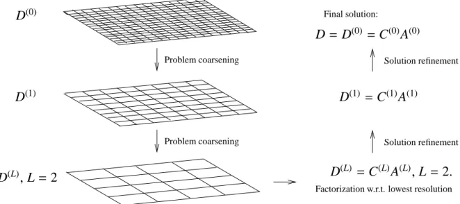
The aim of this paper is to introduce a multiresolution method for the convergence acceleration of a multivariate curve resolution method. The key idea is to utilize a sequence of coarsened factorization problems in order to compute an associated sequence of gradually refined approximations of the solution. The coarsest problem can be solved with relatively low computational costs and provides good starting values for the factorization problem for the next refined resolution level. These two steps of a correction of the solution with respect to a given resolution level together with the subsequent refinement form a “correction-refinement cycle”. This cycle is applied on the sequence of refined grids until a nonnegative matrix factorization of the initial spectral data matrix D is computed, see Figure 1.

1.2. Organization of the paper

The paper is organized as follows: In Section 2 a short introduction to multivariate curve resolution techniques is given which includes the principles of soft- and hard-modeling. The central multiresolution approach is introduced in Section 3. Its application to model data and to experimental data from the rhodium- catalyzed hydroformylation process is presented in Sec- tion 4. Different strategies for the refinement steps are analyzed.

2. Multivariate curve resolution methods

Multivariate curve resolution methods are powerful tools to extract pure component information from spectroscopic data of chemical mixtures. The spectroscopic measurements are recorded in a k×n absorption matrix D with k points in time of measurement along the time axis and n spectral channels along the frequency axis.

Whereas the continuous form of the Lambert-Beer law is given in (1) its discrete matrix form reads

D≈CA+E.

The small error term E collects all measurement errors and nonlinearities. The matrix C ∈ R^k×s of concen- tration profiles and the matrix A ∈ R^s×n of the spectra contain columnwise or rowwise the information on the s pure components. The factors C and A and the spectral data matrix D are componentwise nonnegative matrices.

The mathematical problem is to compute a chemically meaningful nonnegative matrix factorization CA from a given D. The most common way to compute this factor- ization is to start with a singular value decomposition (SVD) of D with the form D = UΣV^T, [8]. If D has the rank s, then the matrix can also be represented by a truncated SVD. This truncated SVD uses only the first s columns of U and V. ThenΣis an s×s diagonal matrix containing the s largest singular values on its diagonal.

With these matrices the desired factors C and A can be constructed with a regular matrix T ∈R^s×sas follows

C=C[T ]=UΣT⁻¹, A=A[T ]=T V^T, (2) see e.g. [16, 15]. Sometimes we write C[T ] and A[T ] in order to express the functional dependence of C and A on T . If the spectral data includes noise, then one can alternatively use a number of z > s left- and right singular vectors. In this case T is an (s×z)-matrix and T⁻¹is substituted by the pseudoinverse T⁺.

2

(3)

Problem coarsening

Factorization w.r.t. lowest resolution Final solution:

D

⁽⁰⁾

D

⁽¹⁾

D

^(L)

, L = 2

D = D

⁽⁰⁾

= C

⁽⁰⁾

A

⁽⁰⁾

D

⁽¹⁾

= C

⁽¹⁾

A

⁽¹⁾

D

^(L)

= C

^(L)

A

^(L)

, L = 2.

Solution refinement Solution refinement

Figure 1: The multiresolution approach for the pure component factorization and with three levels of resolution, see Section 3.

2.1. Soft and hard models

The computation of a specific matrix T which deter- mines a factorization in the sense of (2) suffers from the rotational ambiguity of the solution [1, 2, 14, 18, 25].

Approximation techniques have been developed which aim at a representation of the full range of all feasible, nonnegative factorizations [3, 7, 19, 21, 22, 24].

Here our focus is on the computation of a single so- lution which should fit to the chemical reaction system under investigation in the best possible way. The most common approach in order to favor a single solution is to minimize a weighted sum of regularization functions (soft-modeling) or to apply hard models like a kinetic model. Then the resulting factors C and A are the solu- tions of a numerical optimization process.

For the soft model approach the target function reads F :R^s^×^s→R, T 7→F(T )=

Xp

i=1

γif_i(T )².

If a minimum of F(T ) is taken inT , then Cb = C[bT ] and A=A[bT ]. Therein the p regularization functions fi

are weighted with nonnegative parametersγ_i. Regular- ization functions can be formulated for instance on the nonnegativity of the factors or on their smoothness or unimodality. Typically, the nonnegativity of the factors is the most important constraint so that the associated weight factor is relatively large.

Hard constraints are much more restrictive than soft constraints. Approximately hard constraints can be im- plemented by means of a constraint with a very large

weight factor. An important example of a hard constraint is a kinetic model whose consistency with the solution C is required.

Let K be the vector of the q kinetic parameters and let C^(ode)be the associated solution of the kinetic model.

This allows to compute T =(C^(ode))⁺UΣ(:,1 : s) as well as C=UΣT⁻¹and A=T V^T. Then the function

G :R^q→R: K7→ kC−C^(ode)k^F+pen. terms (3) is taken as a measure how well a kinetic model parametrized with K fits to a nonnegative factorization.

The penalty terms in (3) are used to suppress negative matrix entries. All this results in an optimal fit with the kinetic model [5, 9, 20].

2.2. Computational costs

The costs for the computation of C and A depend on - computational costs for one evaluation of the func-

tion F and

- the number of necessary function calls for its iterative minimization.

In general it holds that s≪k,n so that the dependence of the costs on the dimension parameters k and n is deci- sive. In Section 3.1 of [21] a detailed discussion shows that the computational costs for a proper implementa- tion increase linearly in k+n if a small negative lower bound is used for the acceptable relative negativeness of the factors C and A. Additionally the number of neces- sary iterations for the minimization of F is decisive for 3

(4)

the computational costs of the numerical algorithm. A good initial value can be expected to result in a small number of iterations for the correction.

The multiresolution approach reduces the costs on both fronts: for low-resolution factorization problems the costs for single function calls are relatively small and at each refined level reliable initial values are pro- vided for the iterative minimization.

3. The multiresolution approach for the pure com- ponent factorization

Modern computerized spectroscopic devices can pro- duce considerable amounts of data, e.g. UV-Vis diode array systems can generate several megabyte of data within short time periods. Hence the dimensions k and n of the spectral data matrix D ∈ R^k^×ⁿ can be large and high computational costs are to be expected for a direct nonnegative factorization D = CA of the high- dimensional matrix D.

The general approach for our multiresolution tech- nique for the pure component factorization D =CA ∈ R^k^×ⁿis as follows:

Algorithm: Multiresolution factorization

1. Starting from D = D⁽⁰⁾ a sequence of lower dimensional submatrices D⁽¹⁾, . . . ,D^(L) is gener- ated. These matrices represent D on coarser time- frequency grids, see left side of Figure 1.

2. Compute a pure component factorization D^(L) = C^(L)A^(L)for the coarsest problem of lowest resolu- tion, see right lower part of Figure 1.

3. Prolongate this solution in order to generate ini- tial values of the iterative minimization for the fac- torization problem on the next finer time-frequency grid.

4. Compute the pure component factorization with re- spect to the current grid.

5. Repeat steps 3 and 4 until a factorization D = D⁽⁰⁾ = C⁽⁰⁾A⁽⁰⁾ with respect to the finest grid is determined, see right upper part of Figure 1.

Step 2 for a small matrix D^(L) can be completed rapidly. With a proper prolongation of the solution in step 3 the factorization in step 4 requires few iterations.

In the following we demonstrate that the multiresolution approach can result in a considerable convergence acceleration. However, the whole procedure requires that

the time and frequency discretization parameters (sampling rates) are small enough that they can resolve the signals along the time and frequency axes.

3.1. Sequence of coarsened subproblems

The multiresolution approach requires that the sampling rates along the time axis and the frequency axis are small enough so that the sampled signal can still approximate (by interpolation) the original signal; this prerequisite is related to the Nyquist-Shannon sampling theorem of digital signal processing [23]. The theorem says that the sampling frequency of a signal should be at least twice the maximal frequency of the signal in order to guarantee an exact reconstruction. Practically the time step between two spectra should be small compared to the change of the concentration values and the frequency step should be small compared to the change of the absorption values.

Figure 2 demonstrates that the singular value decomposition is not very sensitive with respect to the data coarsening. To this end we consider the spectral data for the hydroformylation process; the details on this data set are explained in Section 4.3. This data set comes with k=2621 spectra and n=664 wavenumbers. If we use a coarsening only along the time axis and if the submatrices have the dimensions⌈2621/2ⁱ⌉×n for i=0, . . . ,9, then the properly scaled singular vectors of these matrices look very similar and the singular values show only small variations. (In the last sentence the ceiling function⌈q⌉, which is the smallest integer number larger or equal to q, is introduced in Definition 3.1.)

3.2. Notation for the coarsened problems

Next the level indexℓ is introduced in order to enu- merate the different levels of resolution of the factorization problem. This indexℓ is added in brackets to the related matrices, singular value decomposition and to the associated target function. The starting point for the multiresolution approach is the initial spectral data matrix D = D⁽⁰⁾ ∈ R^k×n. The levelℓ = 0 is the level of highest resolution. The levels of coarsened problems areℓ=1,2, . . .L up to a maximal index L.

- The submatrix D^(ℓ)of D represents a sampling with respect to the time and frequency index vectors t^(ℓ) andλ^(ℓ), i.e. D^(ℓ) = D(t^(ℓ), λ^(ℓ)). The vector t^(ℓ) is a subvector of the vector 1 : k = (1,2, . . . ,k) and the vectorλ^(ℓ) is a subvector of the vector 1 : n = (1,2, . . . ,n).

- The SVD of D^(ℓ)reads

D^(ℓ) =U^(ℓ)Σ^(ℓ)V^(ℓ)^T. (4) 4

(5)

0 1000 2000 3000 4000 5000

−0.03

−0.02

−0.01 0 0.01 0.02 0.03 0.04

First 3 left singular vectors

time [min]

0 5 10 15 20

10⁻¹ 10⁰ 10¹

First 20 rescaled singular values

i σi

1980 2000 2020 2040 2060 2080 2100

−0.1

−0.05 0 0.05 0.1 0.15

First 3 right singular vectors

wavenumbers [1/cm]

Figure 2: Rescaled singular values and rescaled singular vectors of D and its submatrices for a coarsening along the time axis. See Remark 3.3 and Equation (8) for the proper scaling.

- The target function for the hard- or soft modeling optimization is denoted by

F^(ℓ):R^p→R (5)

where p is the number of unknown parameters. For the soft-modeling method, see Section 2.1, it holds that p = s² or p = s z and for the a kinetic hard model p is the number of kinetic parameters.

- The sequence of matrices T , see Equation (2), with respect to the coarsening levelℓand the ith itera- tion step is T^(ℓ,i), i = 0, . . . ,Nℓ. The number of iterations on levelℓ is Nℓ. The optimal and final matrix is denotedTb^(ℓ).

- The pure component factors are C^(ℓ) and A^(ℓ). 3.3. Definition of the multiresolution hierarchy

Next we define the hierarchy of subproblems for the factorization problem. For the coarsening it is important that the reduction of the dimension is large enough so that the computing time saving is significant. The reduction should also be small enough so that the solution with respect to a certain levelℓ after its prolongation is a good initial estimate for the levelℓ−1 of the next problem with a higher resolution.

Next the colon notation as well as the floor and ceiling functions are introduced.

Definition 3.1. For an integer number m the notation 1 : m defines the vector (1,2, . . . ,m) of integers. Further 1 :δ: m with the incrementδdenotes the vector (1,1+ δ,1+2δ, . . . ,1+kδ) with the largest possible k so that 1+kδ≤m. For example 1 : 3 : 9 represents the integer vector (1,4,7). Further the floor and ceiling functions are given by

Floor function ⌊x⌋=max{m∈Z: m≤x}, Ceiling function⌈x⌉=min{m∈Z: m≥x}.

The principles of the problem coarsening are as follows:

1. The original spectral data matrix D=D⁽⁰⁾ ∈R^k^×ⁿ can formally be written as

D⁽⁰⁾=D(t⁽⁰⁾, λ⁽⁰⁾) with t⁽⁰⁾=1 : k andλ⁽⁰⁾=1 : n.

2. The different levels of resolution are enumerated byℓ=0, . . . ,L.

3. Two monotone increasing sequences of index increments determine the coarsening process. For the time axis letτbe the vector of increments, and for the frequency axis letχbe the vector of increments. This reads

τ:=[τ₀, τ1, . . . , τL], χ:=[χ₀, χ1, . . . , χL]. (6) Withτ0 =χ0 =1 it is assumed that

τℓ+1

τℓ ∈N, χℓ+1

χℓ ∈N (7)

forℓ=0, . . . ,L−1.

4. For the levelℓlet

t^(ℓ)=1 :τℓ: k, λ^(ℓ) =1 :χℓ: n be sequences of subindexes of 1 : k and 1 : n. (The first index set consists of⌊k/τ_ℓ⌋elements and the second index set of⌊n/χ_ℓ⌋elements.)

5. The submatrix D^(ℓ)is

D^(ℓ)=D(t^(ℓ), λ^(ℓ))∈R^⌊^k/τ^ℓ^{⌋ × ⌊}^n/χ^ℓ^⌋. Example 1. A possible choice for the spectral data ma- trix from Section 4.3 with k=2621 and n=664 is

τ=[1,2,4,8, . . . ,256] and χ=[1,1,1, . . . ,1].

5

(6)

This results in a sequence of eight submatrices of D by taking from levelℓto levelℓ+1 only every second spec- trum and by letting the spectra along the frequency axis unchanged. The nine different matrices including the original data matrix D = D⁽⁰⁾ have the following di- mensions:

D⁽⁰⁾∈R²⁶²¹^×⁶⁶⁴, D⁽¹⁾∈R¹³¹¹^×⁶⁶⁴, D⁽²⁾∈R⁶⁵⁶^×⁶⁶⁴, D⁽³⁾∈R³²⁸^×⁶⁶⁴, D⁽⁴⁾∈R¹⁶⁴^×⁶⁶⁴, D⁽⁵⁾∈R⁸²^×⁶⁶⁴, D⁽⁶⁾∈R⁴¹^×⁶⁶⁴, D⁽⁷⁾∈R²¹^×⁶⁶⁴, D⁽⁸⁾∈R¹¹^×⁶⁶⁴. Definition 3.2. The resolution levelℓtogether with the definitions from above can formally be written as a triplet

S^(ℓ)=

t^(ℓ), λ^(ℓ),D^(ℓ) .

The hierarchy of resolution levels is nested in the sense that

S^(L)≺ S^(L⁻¹⁾≺ · · · ≺ S⁽⁰⁾=

1 : k,1 : n,D⁽⁰⁾ .

The relationS⁽ⁱ⁾ ≺ S^{( j)} is satisfied for i> j if and only if t⁽ⁱ⁾is a subsequence of t^{( j)}andλ⁽ⁱ⁾is a subsequence of λ^{( j)}.

Remark 3.1. The assumptions on the nested sequence of subproblems with S⁽ⁱ⁾ ≺ S^{( j)} implies that D⁽ⁱ⁾ is a submatrix of D^{( j)}. Thus the coarsest matrix D^(L) is a submatrix of D⁽⁰⁾.

3.4. Prolongation and restriction operations for con- secutive resolution levels

Having defined the different levels of resolution for the pure component factorization problem, we still need operations to restrict the problem from one resolution level to the next coarser level and to transfer the result from one level to the next finer resolution level. Fol- lowing the common terminology in multigrid methods [10] we denote these transfer processes as restriction and prolongation operations.

Definition 3.3. A mappingP^(ℓ) : S^(ℓ+1) → S^(ℓ) from a coarse resolution problem to the next finer resolution is called a prolongation. The restriction operation is a mappingR^(ℓ):S^(ℓ)→ S^(ℓ+1).

Remark 3.2. The prolongation and restriction opera- tors should naturally satisfy thatR^(ℓ)◦ P^(ℓ)is the iden- tity operator onS^(ℓ+1). However,P^(ℓ) ◦ R^(ℓ) is usually not the identity operator onS^(ℓ).

We do not only need P^(ℓ) for the prolongation of D^(ℓ+1) to D^(ℓ), but we must also prolongate the factors C^(ℓ+1)and A^(ℓ+1)to the resolution levelℓ. The key point is to execute this prolongation in an implicit manner by considering the associated matrices T , i.e. an initial es- timate for T^(ℓ,0) is computed. Next three different ap- proaches are suggested for the computation of T^(ℓ,0). Definition 3.4. For given factors C^(ℓ+1)and A^(ℓ+1)with respect to the resolution levelℓ+1 three alternative tech- niques for the prolongation to the levelℓare suggested;

this is formally written as a prolongationbP^(ℓ) of C^(ℓ+1) and A^(ℓ+1)to T^(ℓ,0). For each technique a least squares problem is to be solved. Hence,

T^(ℓ,0)=bP(C^(ℓ+1),A^(ℓ+1))=argmin

T φ_i(T ) with optionally (for i=1, 2 or 3)

φ1(T )=A^(ℓ+1)−T M^T₁²_F, φ2(T )=C^(ℓ+1)−M2T⁺²_F, φ3(T )=φ1(T )+φ2(T ) and

M1=V^(ℓ) 1 : χℓ+1

χℓ

:

$ n χℓ+1

% ,1 : z

! ,

M2=U^(ℓ) 1 : τℓ+1

τℓ

:

$ k τℓ+1

% ,:

!

Σ^(ℓ)(:,1 : z).

The first target functionφ1only uses the structure of A, namely A^(ℓ+1) is approximated in the least squares sense by right singular vectors of the higher resolution level. These vectors form the columns of M1. Simi- larlyφ2uses the structure in C in order to construct T⁺ from the augmented left singular vectors composed in M2. Finallyφ3 uses an averaging ofφ1 andφ2. These prolongation strategies can be applied along the time or frequency axis irrespective of whether a resolution coarsening has previously been executed along this axis.

Each of these strategies to find a proper T^(ℓ,0) can be very useful.

Remark 3.3. For a direct comparison of the singular vectors and singular values with respect to different lev- els of resolution one has to take into account their po- tentially differing orientation by a multiplication with

−1. Furthermore, the different dimensions of the singu- lar vectors, which are all normalized with respect to the Euclidean norm, results in the following rescaling

√1τi

U⁽ⁱ⁾, 1

√χ_iV⁽ⁱ⁾, i=0, . . . ,L. (8) 6

(7)

The insertion of columns or rows to D⁽ⁱ⁾also results in a rescaling of the singular values. The simplest way to see this is to consider either (D⁽ⁱ⁾)^TD⁽ⁱ⁾or D⁽ⁱ⁾(D⁽ⁱ⁾)^Twhose roots of the eigenvalues are (at least) the nonzero singu- lar values of D⁽ⁱ⁾. For the singular values the rescaling is

√τ_iχ_iΣ, i=0, . . . ,L. (9) 3.5. Algorithm of the multiresolution procedure

The multiresolution procedure can be applied to any SVD based multivariate curve resolution method in- cluding the matrix T by (2) and regardless of the used regularization. The algorithmic steps are as follows:

1. The multiresolution sequence of matrices D^(ℓ) is determined by fixing the number of resolution lev- els L and the vectorsτ andχ of increments, see Equation (6).

2. On the coarsest level ℓ = L with the lowest res- olution an initial nonnegative factorization D^(L) = C^(L)A^(L) is computed by means of a minimization of the target function F^(ℓ).

3. Then forℓ=L−1,L−2, . . . ,0 the following steps are executed

(a) The prolongationbP^(ℓ) with one of the target functionsφ1, φ2 andφ3 is used in order to compute the initial matrix T^(ℓ,0)on the level ℓ.

(b) The iterative minimization for the target func- tion F^(ℓ) is executed. The minimum is at- tained in the factors C^(ℓ)and A^(ℓ)for the resolution levelℓ.

4. The final solutions are C =C⁽⁰⁾ and A = A⁽⁰⁾ on the levelℓ=0 of highest resolution.

3.6. Benefit of the multiresolution procedure

The multiresolution procedure serves to accelerate the computation of nonnegative factorizations of the spectral data matrix of medium- and high-dimensional data. The computational costs, see Section 2.2, depend on the computational costs for a single step and on the total number of required iterations.

The multiresolution procedure reduces these costs by generating a sequence of coarse resolution approximations, which can each be computed with drastically reduced computational costs. Moreover, the final iterate with respect to a certain resolution levelℓis a good initial estimate for the next resolution levelℓ−1. An effi- cient and fast-converging multivariate curve resolution method can be constructed by a suitable combination of the problem coarsening and the approximate solution of

the low resolution problems. Below the line, computational costs are saved by introducing additional levels of resolution.

One could object that the multiresolution procedure is applied to oversampled data and that any savings of the computational costs originate from reducing the problem to a reasonable level of resolution. To some ex- tent this is true. However, modern computerized spectroscopic instruments usually result in high-resolution data. Then it is not clear a-priori which level of resolution is sufficient in order to extract the desired spectroscopic detail information. To be on the safe side, one usually accepts oversampling and applied the MCR method to the full data set. Further on, poorly resolved data can even allow to compute good initial approximations for pure component factorizations with respect to the next level of resolution. Thus the multiresolution procedure can also work without oversampled data.

3.7. Multiresolution techniques and hard-modeling The underlying idea of the multiresolution procedure can be extended to hard-modeling [5, 15]. To this end the hard model is implanted into each level of resolution. On the coarsest level a first approximation of the kinetic parameters is calculated and these values are used as initial values on the next refined resolution level.

This procedure is repeated level by level. Hence the prolongationPis not needed for the implementation of a hard model. Computationally, the problem is to mini- mize the function G(K) as introduced in (3). This results in a vector K of kinetic parameters so that the associated solution C^(ode)optimally fits C. The computational costs for the solution of this optimization problem depends on the number of function evaluations G(K). The costs for a single function evaluation consist of the computational costs for the ODE solver (these costs are more or less constant and do not depend on the level of resolution) and on the costs for computing the approxima- tion error C−C^(ode)with optimally scaled C^(ode). The costs for the latter computations are proportional to the dimension of the current level of resolution, namely k and n or a fraction of these numbers. This dependence on k and n is the crucial point why the multiresolution approach can accelerate the computations. Once again, good initial approximations for K can be computed on the coarse levels and these results are reused by prolongation on the levels of higher resolution. The number of coarse level iterations has a minor impact on the total computational costs due to the smaller dimensions of D^(ℓ). Finally, on higher levels of resolution only few of the more costly iterations are needed. In Section 4.5 this technique is demonstrated for experimental spectral 7

(8)

0 2 4 6 8 10 0

0.2 0.4 0.6 0.8 1

time Concentration profiles

0 20 40 60 80 100

0 0.2 0.4 0.6 0.8 1

channels Spectra

Figure 3: The pure component factors C and A of the four component model problem from Section 4.2.

data. This leads to savings of about 90% of the computing time.

3.8. Selection of the coarsening increments

A proper selection of the vectors of coarsening increments (6) appears to be decisive for a successful multiresolution procedure. In our experimentsτ orχ be- ing equal to [1,2,4, . . .] always work in a stable way.

In some instances the vector of coarsening increments [1,4,8, . . .] appears to result in an over-coarsening of the problem so that the final iterates cannot result in reliable initial estimates on the next finer resolution level.

However, all this depends on the relation of the amount of data and the variability or dynamics of the data, cf. the discussion in the first paragraph of Section 3.3.

4. Numerical results

4.1. Hard- and software information

All computations have been performed on a PC with an Intel Quadcore 64bit processor with 3.4Ghz and 16GB RAM. Without parallelization only one core has been used for the computations. The program code has been written in C and uses a nonlinear least-squares op- timizer code NL2SOL of the ACM [6] written in FOR- TRAN. For the solution of the initial value problems for ordinary differential equations, which are kinetic hard models in Section 4.3, we use the prominent RADAU IIa codes [11]. The very effective FORTRAN implementation of the RADAU algorithms is available under the web address

http://www.unige.ch/hairer/prog/stiff/radau.f . 4.2. Application to a model problem

Next the multiresolution approach is applied to the consecutive reaction system with s=4 components

A−→^k¹ B−→^k² C−→^k³ D.

The concentration profiles of the four components are determined by the rate constants k1 =1, k2=2, k3=1 and by the initial concentrations (1,0,0,0). The time in- terval t ∈[0,10] is subdivided by k=1001 equidistant grid points. The pure component spectra are Gaussian profiles within the intervalλ ∈[0,100] with n =2001 equidistant grid points. Hence D = CA ∈ R¹⁰⁰¹×2001. The pure component spectra and concentration profiles are shown in Figure 3.

The relatively large dimension parameters k =1001 and n = 2001 indicate that the spectra and concentration profiles are oversampled; cf. the discussion on oversampling in Section 3.6. Thus the acceleration effect of the multiresolution factorization can clearly be demonstrated. Next two coarsening strategies are tested:

1. Simultaneous coarsening in the time and in the frequency direction.

2. Coarsening only in the frequency direction.

For these computations nine different runs of the multiresolution factorization with the numbers L = 0,1, . . . ,8 of resolution levels are used. The computa- tion for L = 0 represents the case of a direct computation of the pure component factorization without any coarsening of the time-frequency grid.

4.2.1. Active soft constraints and evaluation criteria For all computations soft constraints are used on the nonnegativity of the factors C and A. The reconstruction errorkD−CAkFis controlled by evaluatingkI−T T⁺kF

where T⁺ is the pseudoinverse of T . Additionally we use a constraint on the integral of the spectra (where each spectrum is normalized to a maximum equal to 1) in order to favor spectra with a small number of sharp peaks. With these constraints the original factors can be reconstructed in all program runs.

For the purpose of a comparison of the numerical results, the computation times are recorded together with number of inner iterations until termination of the NL2SOL code, see Section 4.1. Moreover, the computation times for all intermediate levels are collected. On the coarsest grid level withℓ=L the computation of a first solution starting from an initial random guess de- cisively influences the computational costs of the optimization algorithm. Typically no good initial estimates are available on the coarsest level of resolution. These can be produced by a genetic algorithm. On all finer levels withℓ < L we only used the Gauss-Newton al- gorithm for the minimization in the form of its sophisti- cated implementation in the NL2SOL code [6].

In order to avoid any influence of poor initial estimates the multiresolution program, including the ge- 8

(9)

netic algorithm, is run 20 times. The two program runs with the highest computation times are ignored, and also the two program runs with the minimal computation times are dropped. For the remaining 16 program runs we tabulate the mean values of the computation times and for the required number of iterations.

4.2.2. Multiresolution factorization in time and in fre- quency direction

First the time-frequency grid is coarsened in each of the coordinate directions. Together with L=9 the vectors of coarsening increments, see (6), are

τ=χ=(1,2,4,8,16,32,64,128,256).

Hence the number of grid points is doubled along the time direction and also along the frequency direction for every transition from one level of resolution to the next refined level. Thus D⁽⁰⁾ = D ∈ R¹⁰⁰¹×2001 and D⁽⁹⁾ ∈ R⁴×8.

Tables 1 and 2 show the mean values for the computation times and the associated numbers of necessary iterations with respect to all intermediate levels of resolution. These data indicate that the multiresolution factorization works very well. The computation times for L = 2, . . . ,8 are about a third of the computation time without any multiresolution computation, i.e. the case L = 0. If for L = 1 only a single grid coarsening is used, then the saving of the computation time are about 50%. The results also show that there are nearly no sav- ing beyond L=2 with D⁽²⁾∈R²⁵¹^×⁵⁰¹.

4.2.3. Multiresolution factorization in frequency direc- tion

The multiresolution factorization can alternatively be applied either to the frequency direction or to the time direction. To demonstrate this, we set the coarsening increments to

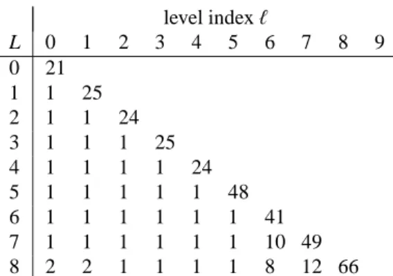
τ=(1, . . . ,1), χ=(1,2,4,8,16,32,64,128,256), which amounts to a coarsening in the frequency direction. The computation times and the numbers of necessary iterations for all intermediate levels are listed in Tables 3 and 4.

For this coarsening strategy the multiresolution fac- torization works best for L =2, . . . ,4 with savings for the computational costs of about 50%. If larger L are used, then the computational costs increase again as no coarsening is applied along the time direction. Then the computational costs suffer from relatively large costs for the prolongation operations and for the refinement iterations which still work with the full resolution along the time direction.

2000 2050 2100

0 0.02 0.04 0.06 0.08

wavenumbers [1/cm]

absorption

Figure 4: FT-IR spectroscopic data from the rhodium catalyzed hy- droformylation process [13]. Only every 50th of the k=2621 spectra is plotted.

4.3. Application to experimental data from the hydro- formylation process

In this section the multiresolution factorization is tested for FT-IR spectroscopic data from the hydroformylation of 3,3-dimethyl-1-butene with a rhodium monophosphite catalyst ([Rh] =3×10⁻⁴mol/L) in n- hexane at 30^◦C, p(CO) = 1.0 MPa and p(H2) = 0.2 MPa; for the details see [13]. Figure 4 shows a sub- set of the sequence of k = 2621 spectra. Each spec- trum has n = 664 channels in the wavenumbers window [1960.1,2120.0]cm⁻¹. In this window the absorption by the reaction product, the aldehyde, is negligible.

A number of s =3 dominant components, namely the olefin, the acyl complex and the hydrido complex, contribute to the absorption in the selected frequency window.

4.3.1. The multiresolution hierarchy

In the first experiment we use soft-modeling with a constraint function which penalizes negative components. We also use a constraint function on the distance of the concentration profiles to the Michaelis-Menten model

S +K k1

GGGGGB F GGGGG

k₋1

[S−K]−→^k² P+K (10) with a simultaneous optimization of the kinetic parameters [20]. The components are the substrate (S), the catalyst (K), the substrate-catalyst complex (S-K) and the product (P). Since the product P does not contribute to the absorption in the selected wavenumbers window, this component is considered in the model but is not a part of the regularization function.

9

(10)

level indexℓ times [s] for

L 0 1 2 3 4 5 6 7 8 all levels

0 24.94 24.94

1 6.97 7.39 14.36

2 5.39 1.52 1.39 8.30

3 5.85 1.20 0.28 0.36 7.69

4 6.46 1.13 0.24 0.07 0.15 8.04

5 5.33 1.22 0.24 0.08 0.02 0.08 6.96

6 5.92 1.26 0.27 0.08 0.02 0.00 0.05 7.60

7 6.99 1.16 0.28 0.09 0.02 0.01 0.00 0.02 8.56

8 5.42 1.32 0.28 0.08 0.02 0.02 0.01 0.00 0.02 7.17

Table 1: Computing times [s] for the self-modeling multiresolution factorization with respect to all levels of resolution. The fastest computation with L=5 needs only 6.96 seconds (mean value). This is more than three times faster than solving the original problem with respect to the level of highest resolution L=0.

level indexℓ

L 0 1 2 3 4 5 6 7 8

0 20

1 1 22

2 1 1 23

3 1 1 1 26

4 1 1 1 2 32

5 1 1 1 2 1 41

6 1 1 1 3 1 2 39

7 2 1 1 4 1 4 2 37

8 1 1 1 3 1 6 6 12 57

Table 2: Numbers Nℓof iterations with respect to the single levels for the minimization of F^(ℓ). A relatively large number of iterations is required only forℓ=L. These iterations are computationally much cheaper with respect to larger level indexesℓcompared to smaller level indexes.

level indexℓ time [s] for

L 0 1 2 3 4 5 6 7 8 all levels

0 25.37 25.37

1 5.45 10.10 15.55

2 4.56 2.06 6.08 12.69

3 5.20 1.71 1.23 5.52 13.66

4 5.19 1.66 1.03 1.00 4.67 13.56

5 4.56 1.63 1.04 0.94 0.95 9.08 18.19

6 5.34 1.68 0.97 0.82 0.77 0.90 7.60 18.07

7 5.40 2.03 0.98 0.84 0.80 0.76 2.72 9.30 22.83

8 5.64 2.08 0.99 0.85 0.80 0.76 2.05 2.76 12.37 28.29

Table 3: Computing times [s] for the self-modeling multiresolution factorization. Grid coarsening is only used along the frequency axis. Best results are achieved for L=2, . . . ,4. A stronger coarsening in the frequency direction without simultaneous coarsening along the time axis turns out to be ineffective.

10

(11)

level indexℓ

L 0 1 2 3 4 5 6 7 8 9

0 21

1 1 25

2 1 1 24

3 1 1 1 25

4 1 1 1 1 24

5 1 1 1 1 1 48

6 1 1 1 1 1 1 41

7 1 1 1 1 1 1 10 49

8 2 2 1 1 1 1 8 12 66

Table 4: Number Nℓof iterations with respect to the single levels for the minimization of F^(ℓ). In all cases a relatively large number of the computationally cheap iterations is required only forℓ=L, whereas forℓ <L in most cases a single iteration is sufficient.

The multiresolution procedure is tested for a grid coarsening only in the time direction and for a simultaneous coarsening in the time and in the frequency directions. The numerical results are presented in the form of mean values as explained in Section 4.2.1.

4.3.2. Multiresolution in time direction

For a grid coarsening only in the time direction we set

τ=[1,2,4, . . . ,2^L], χ=[1,1, . . . ,1] (11) for L=0,1, . . . ,8. The computation times and the numbers of iterations until termination are listed in Table 5 and Table 6. The results show an acceleration of the computation by a factor of about 5 for a multiresolu- tion computation with L = 6. These results are to be compared with the case L=0 which corresponds to the standard multivariate curve resolution method without any multiresolution acceleration. The numerical data on the numbers of required iterations show for increas- ing L that the numbers of the computationally expensive iterations on levels with small indexesℓare decreasing.

For L≥1 not more that six iterations are required on the levelℓ=0. This expresses the accelerating effect of the multiresolution factorization: A relatively large number of iterations is only used on the coarsest levelℓ=L of the lowest resolution. For all other levels N_ℓ is much smaller since a reliable initial estimate from the coarser levels results in a relatively small number of iterations.

These results clearly indicate the acceleration effect of the multiresolution procedure.

The computational results for all resolution levels for the case L=8 are shown in Figure 5. The variations of the different curves are small. This demonstrates that the submatrix D^(L) of D for the coarsest level allows

an acceptable approximation of the ”true” solutions for D=D⁽⁰⁾.

4.3.3. Multiresolution in time and frequency directions For a simultaneous grid coarsening along the time direction and the frequency direction we set

τ=[1,2,4, . . . ,2^L] and χ=[1,2,4, . . . ,min(16,2^L)]

for L =0,1, . . . ,8. With these vectors of index increments the grid coarsening along the frequency direction is stopped forℓ≥5. Together with n=664 this selection guarantees that always a minimum of 42 absorption values are used for the computations. The computation times and the numbers of iterations until termination are listed in Table 7 and in Table 8.

Once again the numerical results show an acceleration of the computation by a factor of about 5. All these results are to be compared with the case L = 0 which corresponds to the standard multivariate curve resolution method without any multiresolution acceleration.

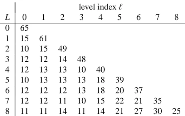
The interpretation of the numbers of iterations is very similar to that given in Section 4.3.2. We conclude that the two coarsening strategies work very well. The saving in the computational time for the given spectral data with k = 2621 separate spectra and n = 664 spectral channels for each spectrum are primarily determined by the coarsening along the time direction.

4.4. Convergence history

For an effective numerical minimization of the func- tions F^(ℓ) our program code uses the adaptive nonlinear least-squares minimization algorithm NL2SOL, cf. Section 4.1. The convergence history is monitored 11

(12)

L 0 1 2 3 4 5 6 7 8 all levels

0 53.90 53.90

1 5.63 16.03 21.66

2 6.01 2.85 4.99 13.85

3 8.70 2.62 0.91 1.41 13.64

4 9.23 2.13 0.77 0.43 1.23 13.78

5 7.07 2.61 0.89 0.50 0.64 1.29 13.01

6 6.16 2.38 0.76 0.36 0.56 0.71 0.54 11.49

7 8.67 2.21 0.69 0.61 0.55 0.37 0.32 0.37 13.81

8 6.80 2.05 0.62 0.33 0.39 0.38 0.25 0.31 0.58 11.71

Table 5: Computation times [s] for the soft-modeling multiresolution procedure for each level. The last column contains the total times for the different L. The fastest computation with L=6 levels of resolution needs only 11.49 seconds. This is about 20% of the total computation time for solving the original problem with respect to level of highest resolution (L=0).

level indexℓ

L 0 1 2 3 4 5 6 7 8

0 37

1 3 39

2 4 6 40

3 6 6 7 26

4 6 5 6 7 35

5 5 5 6 9 18 50

6 4 5 5 6 16 27 24

7 6 5 5 11 15 13 13 17

8 5 5 5 6 11 13 10 14 37

Table 6: Numbers Nℓof iterations for the minimization of F^(ℓ)for each levelℓ=0, . . . ,L for the case of soft modeling. In all but one the largest number of iterations is used on the coarsest level of resolutionℓ=L. These data clearly indicate that the multiresolution procedure accelerates the computation. For L=0 a number of 37 iterations on the finest level with high computational costs is needed. For L=1 only 3 iterations on the finest level are required together with 39 (computationally much cheaper) iterations on the levelℓ=1.

0 1000 2000 3000 4000 5000 0

0.2 0.4 0.6 0.8

Conc. profiles olefin

concentration[mol/L]

time [min]

0 1000 2000 3000 4000 5000 0

1 2 3

x 10⁻⁴ Conc. profiles Rh complexes

time [min]

1980 2000 2020 2040 2060 2080 2100 0

Pure component spectra

wavenumbers [1/cm]

Figure 5: Concentration profiles and spectra for the pure components with respect to all levels of resolution for a computation with L=8. The color assignment is as follows: Red - olefin, blue - acyl complex and green - hydrido complex.

12

(13)

L 0 1 2 3 4 5 6 7 8 all levels

0 53.90 53.90

1 5.40 12.79 18.19

2 7.46 2.13 3.61 13.20

3 8.97 2.02 0.60 0.89 12.49

4 9.80 1.86 0.84 0.42 0.44 13.37

5 7.51 2.14 0.80 0.27 0.33 0.28 11.34

6 8.01 2.45 0.75 0.33 0.24 0.13 0.11 12.02

7 6.83 2.52 1.03 0.43 0.24 0.09 0.06 0.07 11.27

8 8.72 2.17 0.48 0.27 0.19 0.13 0.07 0.04 0.10 12.17

Table 7: Computation times [s] for the soft-modeling multiresolution factorization with grid coarsening along the time and along the frequency axis.

The fastest computation with L=7 levels of resolution needs only 11.27 seconds (mean values), which is a considerable acceleration compared to a direct factorization with respect to level of highest resolution (L=0) with 53.90s.

level indexℓ

L 0 1 2 3 4 5 6 7 8

0 37

1 3 33

2 5 5 36

3 6 5 5 25

4 7 4 7 12 30

5 5 5 7 7 21 39

6 5 5 6 9 15 17 24

7 4 6 9 12 15 12 10 23

8 5 5 4 7 12 17 13 10 33

Table 8: Numbers Nℓof iterations for the minimization of F^(ℓ)for each levelℓ=0, . . . ,L. In all cases the largest number of iterations is used on the coarsest level of resolutionℓ=L. For largerℓthe computational costs for the computation of the initial approximation are considerably decreasing.

13

(14)

by means of two error measures. On the one hand the squared target function

eℓ,j=1

2F^(ℓ)(T^(ℓ,^j))²

is traced for ℓ = L, . . . ,0 and for every ℓ with j = 0, . . . ,Nℓ. On the other hand the distance of the iterates T^(ℓ,^j)to the final matrixTb^(ℓ)at the end of the iteration

fℓ,j=T^(ℓ,^j)−bT^(ℓ)_F

is recorded for ℓ = 0, . . . ,L and j = 0, . . . ,Nℓ −1.

Thereink · k^F is the Frobenius norm.

Figure 6 shows the convergence history for the case of grid coarsening only along the time axis for L =6.

Especially on the coarsest levelℓ=6 with 38 iterations the convergence history shows a significant decrease of the error. For the prolongated problems on the levels ℓ=5, . . .0 the reduction of the errors is relatively small.

4.5. Hard-modeling and multiresolution

In Section 3.7 the principles of a combination of a hard model and the multiresolution approach are explained. Next this is demonstrated numerically. The vectors of increments areτ =[1,2,4, . . . ,2^L] andχ = [1,1, . . . ,1] which are the same values as in Section 4.3.2. On each level the problem is forced to be con- sistent with the kinetic hard model and the results in the form of three kinetic parameters are used as the initial values for the next finer level of resolution. In nine different numerical experiments the numbers of levels are L=0, . . . , L=8. For L=0 the kinetic parameters are computed with respect to the problem of highest resolu- tion, and for L=8 the coarse grid solutions are used in 8 cycles as initial values for the next higher resolution problem. For each of these experiments additionally a genetic algorithm has been used for the first steps on the coarsest level in order to solve the optimization problem in a fast and reliable way.

Figure 7 shows the solutions C^(ℓ) and A^(ℓ), ℓ = 1, . . . ,L, for the experiment with L = 8. The solutions show only small variations which indicates that even the coarsest level of resolution provides a sufficient approximation of the problem. Table 9 contains the computation times for nine different program runs with L=0, . . . ,8. The computation times for the single levelsℓ=0, . . . ,L are listed rowwise. The fastest com- putation for L = 7 needs only 2.79 seconds compared to 26.64 seconds for the original problem on the finest level of resolution.

Finally Table 10 presents the numbers of iterations required for L=0, . . . ,8 andℓ =0, . . . ,L. Once again

this clearly indicates that the multiresolution procedure is a successful strategy for the convergence acceleration.

5. Conclusion

Multigrid, multilevel and multiresolution methods are effective numerical algorithms for the solution of a range of high-dimensional optimization and related problems. In the present paper a multiresolution approach to the solution of pure component factorization problems for bivariate spectral data sets has been presented. This algorithm can considerably accelerate the convergence for medium- and high-dimensional spectral data sets. The method has successfully been applied to multivariate curve resolution methods including soft and hard models.

Perspectively, multiresolution techniques can also be applied to the complicated and costly computations of the area of feasible solutions (AFS), see [7, 21]. How- ever, such an area of application is not straightforward and requires further investigations and the development of proper numerical tools.

References

[1] H. Abdollahi and R. Tauler. Uniqueness and rotation ambigui- ties in Multivariate Curve Resolution methods. Chemom. Intell.

Lab. Syst., 108(2):100–111, 2011.

[2] M. Akbari and H. Abdollahi. Investigation and visualization of resolution theorems in self modeling curve resolution (SMCR) methods. J. Chemom., 27(10):278–286, 2013.

[3] O.S. Borgen and B.R. Kowalski. An extension of the multivari- ate component-resolution method to three components. Anal.

Chim. Acta, 174:1–26, 1985.

[4] Philippe G. Ciarlet. The finite element method for elliptic prob- lems. North-Holland Publishing Co., Amsterdam, 1978. Studies in Mathematics and its Applications, Vol. 4.

[5] A. de Juan, M. Maeder, M. Mart´ınez, and R. Tauler. Combining hard and soft-modelling to solve kinetic problems. Chemometr.

Intell. Lab., 54:123–141, 2000.

[6] J. Dennis, D. Gay, and R. Welsch. Algorithm 573: An adaptive nonlinear least-squares algorithm. ACM Transactions on Math- ematical Software, 7:369–383, 1981.

[7] A. Golshan, H. Abdollahi, and M. Maeder. Resolution of Rota- tional Ambiguity for Three-Component Systems. Anal. Chem., 83(3):836–841, 2011.

[8] G.H. Golub and C.F. Van Loan. Matrix Computations. Johns Hopkins Studies in the Mathematical Sciences. Johns Hopkins University Press, 2012.

[9] H. Haario and V.M. Taavitsainen. Combining soft and hard modelling in chemical kinetics. Chemometr. Intell. Lab., 44:77–

98, 1998.

[10] W. Hackbusch. Multi-grid methods and applications. Springer series in computational mathematics 4. Springer, Berlin, 1985.

[11] E. Hairer, G. Wanner, and S. P. Nørsett. Solving ordinary differ- ential equations I, 2nd edition. Springer, 2002.

14

(15)

0 10 20 30 10⁻³

10⁻² 10⁻¹ 10⁰ 10¹ 10²

level l=6 level l=5 level l=4 level l=3 level l=2 level l=1 level l=0 F^(ℓ)convergence by eℓ,j−eℓ,Nℓ

iteration index eℓ,j

0 10 20 30

10⁻¹⁰ 10⁻⁵ 10⁰

Convergence of T^(ℓ,^j)by fℓ,j

iteration index fℓ,j

Figure 6: Convergence history for the error measures eℓ,j−eℓ,N_ℓ (left) and fℓ,j (right) for a problem with L=6 coarsened levels. The main convergent process can be seen on the coarsest levelℓ=6.

0 1000 2000 3000 4000 5000 0

0.2 0.4 0.6 0.8

Concentrations olefin

time [min]

0 1000 2000 3000 4000 5000 0

1 2 3

x 10⁻⁴ Concentrations Rh complexes

time [min]

1980 2000 2020 2040 2060 2080 2100 0

Spectra

wavenumbers [1/cm]

Figure 7: Hard-modeling solutions. The concentration profiles and spectra for the pure components are plotted for the levelsℓ=0,1, . . . ,L=8.

The color assignment is as follows: Red - olefin, blue - acyl complex and green - hydrido complex. The black dashed lines are the solutions of the kinetic model.

L 0 1 2 3 4 5 6 7 8 all levels

0 26.64 26.64

1 1.11 13.51 14.63

2 0.85 0.58 7.49 8.91

3 0.94 0.49 0.31 3.87 5.62

4 0.91 0.52 0.28 0.14 1.92 3.76

5 0.82 0.52 0.30 0.19 0.14 1.27 3.23

6 0.90 0.51 0.29 0.19 0.14 0.10 0.89 3.01

7 0.89 0.49 0.25 0.16 0.12 0.11 0.08 0.68 2.79

8 0.87 0.49 0.30 0.18 0.12 0.10 0.10 0.09 0.63 2.88

Table 9: Computation times [s] for the hard-modeling approach and for nine different program runs for L=0, . . . ,8. The computation times for the single levelsℓ=0, . . . ,L are listed rowwise. The fastest computation for L=7 needs only 2.79 seconds compared to 26.64 seconds for the original problem on the finest level of resolution.

15