A Multivariate Approach for the Biometrie Comparison of Analytical Methods in Clinical Chemistry

(1)

Feldmann, Schneider, Klinkers t and Haeckeh Multivariate comparison of analytical methods 121 J. Clin. Chem. Clin. Biochem.

VoL 19,1981, pp. 121-137

A Multivariate Approach for the Biometrie Comparison of Analytical Methods in Clinical Chemistry By U. Feldmann, B. Schneider, H. Klinkers t

Medical School Hannover, Department of Biometrics and Medical Informatics and A Haeckel

Medical School Hannover, Institute for Clinical Chemistry (Received July 8/October 27,1980)

Summary: The structural relationship model is recommended for the comparison of analytical methods in clinical chemistry. This model is based on the partition of the observed measurements of the different methods in 2 hypo- thetical random variables: the "expected values", which represent the correct value of the analyte with no error of measurement, and the "error term" representing the measurement errors. It is assumed, that both these variables are normally distributed.

There exists a linear structural relation between different analytical methods for the same analyte, provided the correlation coefficient between each pair of the expected values of these methods is 1. This linear structural relation- ship is expressed by the mean values ^ and standard deviations aj of the expected values, whereas the standard devia- tions of the error terms determine the precision of the methods. As a measure of the precision the coefficient of determination R? is recommended.

The model of structural relationship is an extension of the well known regression models and gives a more realistic approach to the comparison of 2 or more analytical methods. With 2 methods the standardized principle component should therefore replace the regression analysis. The slope of this principle component is identical with the ratio s^y/s^x. Statistical methods for the estimation and for tests of hypotheses of the parameters are derived and demonstrated with an example.

Multivariate Verfahren zum biometrischen Vergleich analytischer Methoden in der Klinischen Chemie

Zusammenfassung: Zum Vergleich verschiedener analytischer Bestimmungsmethoden in der klinischen Chemie werden die Stniktürrelationsmodelle empfohlen. Diese Modelle basieren auf einer Zerlegung der beobachteten Werte in zwei hypothetische Zufallsgrößen: die ^erwarteten Werte", die den korrekten Wert des Analyts repräsentieren, wenn dieser ohne Meßfehler gemessen werden könnte, und die „Fehlerterme", die Schwankungen aufgrund von Geräte- oder Meßfehler repräsentieren. In den Modellen wird im allgemeinen angenommen, daß beide Zufallsvariablen normal- verteilt sind.

Das Vorliegen einer linearen Strukturrelation ist bei der Annahme der Normalverteilung äquivalent mit der Annahme, daß die erwarteten Werte von je zwei Verfahren streng miteinander korreliert sind; d. h. daß der Korrelationskoeffi- zient zwischen den beiden erwarteten Werten l ist. Diese lineare Strukturrelation kann durch die Mittelwerte · und die Standardabweichungen ct{ der erwarteten Werte vollständig beschrieben werden. Die Standardabweichungen der Fehlerterme charakterisieren die Präzision der jeweiligen Methoden. Als ein quantitatives Maß für die Präzision wird der Bestimmtheitskoeffizierit Rf empfohlen, der als l - -\ definiert ist ( ? ist die Varianz des Fehlerterms und ö\?

<*

die Gesamtvarianz der Meßgrößen des Verfahrens Nr. i).

Die Strukturrelationsmodelle bilden eine Erweiterung der bekannten Regressionsmodelle und geben eine realistischere Basis für den Vergleich von zwei oder mehr analytischen Meßverfahren. Bei einem Vergleich von zwei Meßverfahren ist die lineare Strukturrelation (unter Annahme einer Normalverteilung) aus den Meßwerten nicht eindeutig zu identi- fizieren. Es muß vielmehr noch eine zusätzliche Nebenbedingung eingeführt werden, die im allgemeinen darin besteht, daß für das Verhältnis der beiden Fehlervarianzen ein fester Wert vorgegeben wird. Besondere Bedeutung für die An-

0340-076X/81 /00l 9-0121 $02.00

(2)

122 Feldmann, Schneider, Klinkers f and Haeckel: Multivariate comparison of analytical methods wendung besitzt die sogenannte standardisierte Hauptkomponentenmethode, bei der angenommen wird, daß dieses Verhältnis der Varianzen gleich der Neigung der Strukturgeraden ist. Diese Neigung kann dann einfach durch den Quotienten der beiden Standardabweichungen s^y/s^x geschätzt werden. Dieses Verhältnis ist besser geeignet, den Zu- sammenhang zwischen zwei Meßgrößen zu beschreiben, die beide zufällig schwanken, als der übliche Regressions- koeffizient.

In der Arbeit werden statistische Methoden referiert und teilweise neuentwickelt, die das Schätzen von Strukturrela- tionen und Tests über Hypothesen solcher Relationen auch in komplexeren Situationen (allgemeine Zusammenhänge zwischen mehreren Veränderlichen) gestatten. Die Methoden werden an einem Beispiel demonstriert.

1. Introduction

In clinical chemistry the number of analytical methods for measuring the value of the same chemical substance is increasing. To compare these different methods'statistical methods are necessary, which give objective information on the precision and comparability of the various measurements. Often the methods of statistical regression analysis are used to solve this problem. But these methods have the disadvantage that in a pairwise comparison one of the measurements must be considered to be free of random errors. The regression line can depend greatly on the choice of this measurement (as "independent variable"). Therefore the methods of regression analysis cannot be considered as adequate for the comparison of analytical measurement methods, which are in general all influenced by random errors (see I.e. (1-6)).

It seems th&tDeming (7) was one of the first to intro- duce a statistical approach for the comparison of analytical methods in chemistry, which was not based on the assumption of the regression model. This approach was derived by Deming with geometric considerations and based on the principle of minimizing the orthogonal distance between the observed measurements and the estimated straight line (orthogonal mean square regression, see I.e. (8)). It can be shown that this principle is a specific feature of more general statistical methods, called structural relationships. These methods were originally introduced by Karl Pearson (9) and later dis- cussed in different connections by several authors (see e.g. Lei (10-18)). This approach is the adequate statistical way to compare two or more analytical values for the same analyte, where all measurements are influenced by random errors.

In this paper we will give an introduction to this approach and show its important role in clinical chemistry.

The structural relationship will be demonstrated by· . comparing different analytical methods for the measurement of serum cholesterol. The relation to the regression analysis will be shown. Maximum likelihood estimates for the parameters (which characterize the dependence and precision of the different measures) and tests of hypothesis on these parameters (with or without constraints) are derived. The methods can be immediately extended to more complex relationships between the measurements or a more complex structure of the

random errors (e.g. hierarchical or factorial random effect models). They include the methods of factor analysis and path coefficient analysis (see I.e. (10, 19-24, 17, 5)).

2. The structural relationship approach for the comparison of 2 methods

2.1 The model

Let us assume that we have n samples of serum, drawn at random and independently from a population. In each of these samples an analyte is measured by two different methods, giving the measured values x⁴ and yi for the i-th sample. These measurements are realizations of a pair of random variables (X, Y) representing all possible pairs of values which can be measured in the population of all possible samples and measurements. As a basic model assumption the variation of these values is considered as additively composed of two components:

— the variation of the analyte within the population of all possible serum samples,

— the variation of the results in repeated measurements of the same serum sample.

The second variation is due to analytical errors. If such errors did not exist, each repetition of the measurement of the same sample would result in identical values. We call these values the "expected values" of the analyte in the sample and denote it by x* and y\ for the i-th sample.

The residuals between the measured sample values xj and yi and the corresponding expected values x[ and y\

indicate the analytical errors and are denoted by di and ej. So we have the partition of the observed measurements in "expected values" and "error terms":

Yi = y + ej.

The expected values x£ and y\ vary within the population of all possible samples. So they can be considered1 as realizations of random variables X* and Y*, which represent the variation of the expected values within this population. We denote the mean values of these random variables by * and and their variances by a* and £.

These variances indicate the variation of the expected values within the population of all possible samples and are therefore characteristics of this biological population.

J. Clin. Chem. Clin. Biochem. / Vol. 19, 1981 / No. 3

(3)

Feldmann, Schneider, Klinkers t and Hacckel: Multivariate comparison of analytical methods 123 The error terms dj and ej vary within the population of

repeated measurements of the same sample. We assume that this variation is the same for all samples and can be represented by random variables D and E, from which the dj and ej are independent realizations. We assume that these random variables have mean values 0 and variances ë* and Xy resp. Furthermore, we assume that the error terms are mutually independent, independent from the random variables of the expected values and independent for different samples.

From these assumptions we conclude that the observed measurements Xj and yi are realizations of two random variables X and Õ with the mean values ì÷ and £iy (as the expected values) and the variances:

The expected values x* and y* indicate the correctness of the methods (if they agree with the proposed correct values for the sample), and the error terms dj and % the precision. An adequate relative measure of the precision is the coefficient of determination R* or Ry , which presents that part of the total variance ó\ or ó£ , which

is determined by the variation of the expected values within the population of all possible samples, i.e.:

Rï^{2 _ _ *}_{x ~ 2}

Οχ Οχ²

the precision of the methods, which can be expressed by the coefficient of determination as defined above.

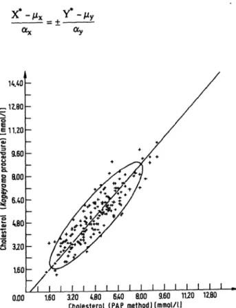
To get estimates for the two parameters 00 and |31 and a further insight in the structural relationship, additional assumptions on the probability distributions of the expected values and error terms are necessary. As usual in statistics, we assume that both the expected values X*, Y* and the error terms D, E have normal distributions with the parameters defined above. Then the random variables ×, Õ of the observed measurements have a bivariate normal distribution with the mean values ì^÷, ì^í, the variances ó*, Oy and a correlation pxy determined by the structural relationship equation. In the x-y-plane the observed measurement values (xj, yj) are scattered like ellipses, as shown in figure 1 for 2 methods for the determination of the cholesterol concentration (obtained from I.e. (25)). These ellipses are called "dispersion ellipses" or "probability ellipses". The borderlines of these ellipses are the curves of constant probability density.

The structural relationship between the expected values X* and Y* implies that the bivariate normal distribution of these random values is degenerate, all the statistical mass being concentrated on a straight line, which of course must be the structural relationship-line (see I.e.

(8)).

The implicit equation of this line is given by:

"

If there are no measurement errors, the corresponding coefficient of determination is 1. In this case the corresponding error variances ë÷ or Xy are 0. If there is no variation of the expected values (o£ or Oy equal zero), all the variation of the observed measurements is due to measurement errors. Therefore the coefficient of determination is 0 in this case.

As both the analytical methods measure the same sample, there must be a relation between the expected values of the methods. We assume that this relation is a linear one and holds for all samples of the population. So we have:

y* = âü + j31 ÷* for all values of i,

where j?0 is the intercept and j3t the slope (to the x-axis) of the corresponding straight-line,

As this linear relation holds for all possible samples, it must hold with probability one for the random variables:

.Y* - 0o probability one.

This is the structural relationship equation for the two measurement methods. It combines the expected values of both methods and allows the prediction of the value of one measurement by knowing the value of the other one in a sample. The accuracy of this prediction depends on

0.00 1.60 3.20 4.80 6AO ROO 9.60 11.20 12.80 Cholesterol (PAP method Hmmol/1J

Fig. 1. Scattergram of the observed points (Xj, Xf) with principal component and dispersion ellipse. The data are taken from I.e. (14). PAP means a commercially available Trin- (fer-method for determining the cholesterol concentration in serum samples.

J. Clin. Chem. Clin. Biochem. / Vol. 19,1981 / No. 3

(4)

124 Feldmann, Schneider, Klinkersf and Haeckel: Multivariate comparison of analytical methods where ì÷ and ìí are the mean values and ax, ay the

standard deviations of the expected values in the population of all samples. This shows that the intercept j3⁰ and slope 0^º of the structural relationship equation can be expressed uniquely by the mean values and standard deviations of the expected values:

This means that the structural relationship equation goes through the point of inertia (ì^÷, ì^ã) with a slope (except for the sign) given by the ratio of the two standard deviations of the expected values (i.e. — for the slope to theOfy

á^{÷ a}*

x-axis and — for that to the y-axis). As the structural

OLy

relation equation is unique, it can be inverted to predict

\l from given y\ :

2.2 The problem of unidentifiability and its solutions

These relations show an intrinsic difficulty of the structural relationship approach for 2 measurements assuming normal distribution: There are only 5 estimable characteristics of the observable measurements X and Õ (ì÷ , ìã , ó^÷, Oy and /o^xy), but 6 unknown structural relationship parameters (ì^÷, ì^ã, á^÷, a^yj ë^÷ and X^y).

So in general the structural relationship parameters cannot be identified by the observable pairs of measurements.

To overcome this difficulty several approaches are possible:

a) Assumption of nonnormality

The assumption of a bivari te normal distribution for both measurement variables is replaced by other assumptions. There are two approaches discussed in the literature:

with

Due to the linear structural relation between the expected values, the random variables of the observed values X and Õ are correlated. Their covariance is given (except for the sign) by the product of the two standard deviations ax and ay of the expected values1); the correlation coefficient is:

= ±·

^'OLy

(where the sign is determined by the sign of the real correlation between the two random variables).

So we see, that the following relations hold between the second-order central moments of the random variables X, Õ and the structural relationship parameters:

= °y =

*) This follows from:

cov(X, Y) =

€(×-ì÷) (Õ -ì÷) = e(X* -ì÷ + Å) (Õ* -My + D) =

= e[(X* - ì÷ + Å) (± ^ (×* - ì÷) + D)) = ± J €(×* - Ì÷)2 ±

± ^ e[E(X* - ì÷)1 + e[D(X* - ì÷)] + e(ED) = ± ay á÷

÷

(since Å, D, ×* are assumed as mutually uncorreiated). The operator e means "expectation" (i.e. e(X) = /xdF(x)).

- Estimation via cumulants

This approach was introduced by Geary (13) and Reierstfl (17). It is based on the observation that the structural relationship involves linear relations between the cumulants of higher order (higher than 3) of the bivariate distribution. These cumulants or semi-invariants are characteristics of the distribution function uniquely related to the moments of the distribution (see I.e. (8), chapter 15.10). They can be estimated by the appropriate sample moments.

By these relations the slope /Jt of the structural relationship line can be expressed as a function of the higher cumulants and therefore estimated by inserting in this function the estimated cumulants (or moments). The problem with this approach is that there is no unique relation between i and the cumulants; choosing differ- ent cumulants (of order higher than 3) results in different estimates for fa. Geary suggests that cumulants of lowest order be used because of ease of computation. This would impose the rather strict assumption that the higher order cumulants are zero, which would be an

objection to many practical situations. Other authors try to pool estimates of fa based on different cumulants to get estimates of minimum variance. But this minimum depends on the exact form of the distribution function and may fail if the assumptions underlying the method are not correct. For details the interested reader is referred to I.e. (14).

- Estimating by grouping

This method in simplest form consists of ordering the observed pairs (X|, yi) in some manner, selecting propor- tions pt and p2 such that P! + p2 < 1 (e.g. pt = p2 = 1/3), placing the first rip-j pairs in one group G^ and' the last np² pairs in another group G² (discarding the middle

J. Clin. Chem. Clin. Biochem./ Vol. 19, 1981 /No. 3

(5)

Feldmann, Schneider, Klinkers f and Haeckel: Multivariate comparison of analytical methods 125 group of observations if pt + p2 < 1) and estimating the

slope 0^t of the structural relationship line by the quotient of the weighted group-mean-differences of the y{ and Xj values; i.e. by:

l Ó -1 Ó

P 2 i e G2

- Ó

ieG,

-çÑ2 ieG Ó Xi)a

(if Pi = ñ²; e.g. both are 1/3, this formula reduces to the ratio of the differences between the group-sums of the y⁴ and X^A values).

The problem is to choose an ordering manner which yields consistent and optimal estimation. This problem was treated by Wald (26\Neyman & Scott (27), and Wolfowitz (28,18). A simple way would be to order the pairs (x$, yO according to the rank of the Xi-values. But then rather complicated and unrealistic assumptions about the distributions of the pairs (Xj, y4) must be made, if the estimate b is to be a consistent estimate (seeMadansky (14)). Also other ordering rules lead to rather complicated conditions for the distribution of the measurement pairs, which are hard to realize and practic- ally impossible to improve.

So as a summary of the discussion on the nonnormal approaches we citeMoran (15), p. 235): "These results are theoretically very complicated and not very useful in practice since it is only in very rare situations that we can be sure that the underlying distribution . . . is nonnormal. It is also natural to expect that the closer this distribution approaches normality the more ineffective any such method of estimation will become." We will not further discuss this approach and refer the interested reader to the cited literature.

b) Repeated measurements

One gets independent estimates for ë÷ and Xy by re- peating the measurements on the same samples p-times (e.g. twice or three times). So one gets pairs of measurements (Xjj, yjj), where the first index is the number of the sample (i = 1,..., n) and the second one the number of repetition (j = 1,..., p). If the repeated measurements can be considered as realizations of independent random variables, having for each sample the same variance ë÷ or ëã, estimates for these variances are:

where xi = i Ó ÷« and yi = - Ó y^u are the arithmetic ' P j Ñ j

means for the ivthe sample.

If the measurements are repeated twice (double measurements) these formulas reduce to:

12 =

2n 2(yii-yi2)2

Tn

Estimates for the total variances ó2 and ó2, are:

— 1 _ 1

where x.. = — Ó xy and y„ = — Ó y^- are the overall means.

From this one gets as estimates for the variances a£ and

2 .2 _ ò2 é2

dy sy Ay

and for the slope |3á of the structural relationship equation:

(where the sign is the same as for the estimated covariance between X and Y).

In general these estimates a£ and ay will not fit the third relation, which reads in estimates:

^ · ^ · r = a · Λ

*>÷ by rxy ax ay

where r^xy is the sample correlation of X and Y.

As the analytical errors of the measurements within an analyte sample are supposed as uncorrelated, this sample correlation is given by the correlation between the sample means of the two measurements within the repeated measurements of the analyte samples:

r^xy =

11

Ó (x^f. - x..) (y^{. - y..)/s^x

Using this sample correlation and the relation ahead one gets as estimate of the slope â^ :

¼ = 2 2

xy

This estimate is in general different from the first one;

both are consistent (i.e. they converge for increasing ç to the true parameter j3^t) but not efficient estimates (estimates with at least asymptotic smallest variance).

Madansky (14) has shown, that the whole problem can be treated as a variance component problem, where the total variance and covariance of the two measurements is J. Clin. Chem. Clin. Biochem. / Vol. 19,1981 /No. 3

(6)

126 Feldmann, Schneider, Klinkers t and Haeckel: Multivariate comparison of analytical methods decomposed in the variation between the analyte

samples and within the repeated measurements of the sample. These variance components generate additional consistent, but not efficient estimates for ft.

The problem is to make an appropriate choice of the

"best" of these consistent estimates. This problem, which is known as "overidentification" problem was discussed by Barnett (11) and Kiefer (29), who showed that an efficient estimate can be obtained by introducing the estimates l^x and I² (together with the estimates s², s2 and rxy derived above) into the maximum likelihood equation and solving it with respect to ft. This leads to the estimate bt given in table 1 for the constraint

£v2 _ i2/i2 W - lyMx-

It should be mentioned that a unique consistent and efficient estimate of ft is possible, if only one of the measurements is repeated. If e.g. only the xy-measurements are repeated, one can directly estimate l| and get an efficient estimate of ft:

, _^sx^sy^rxy

b l" ,2 ,2

sx lx

If the y-measurements are repeated (yy) the residual variance ly can be directly estimated and the estimate of ft is:

s? -I2

_ Sy - i y

The estimates of the sample correlation rxy are:

1 __

n -1 j

if measurement ÷ is repeated

if measurement y is repeated.

c) Constraints on the error-variances

The approach mostly used to overcome the unidentifiability problem is to impose constraints on the structural relationship parameters. There are several types of such constraints possible, two of which are of particular importance:

The//m type of constraints assumes either ë^÷ or X^y equal to 0. This means, that either the first or the second measurement method is free of measurement errors. It is analogous to the assumptions in regression analysis and reduces the structural relationship model to the corresponding regression models:

Xi = + f t y i + di if X^y= 0 .

But there is an important difference between these models and the usual regression analysis. Whereas in the

Tab.l. The slope bt and the standard deviations of random errors lx, ly are given in terms of the standard deviations sx, sy and the correlation r of the two observed measurements.

The constant c<i in principle component analysis is given by: GI - + >/(Sy - sx) + 4r2 · sx · sy

The constant C2 in the model with constraint \y/\x = È2 is given by: c2 - Vis2, - È2 sx)2 + 4È2 r2 sx Sy Statistical

analysis Slope of linear relationship Standard deviation of random error

Measurement ÷ Measurement y

l l

Regression ù (÷ independ-

•g ent) ID Regression

(y independent)

r - s^y

sy

r · sx n - 2-.

n - 2

Principle a> component

.2

Standardized principle component

r IrT

-? 2

'-Ars_n-1 ².(l-l Constraint

\y/\^x = È² ^"^{2 2 2} -^^(202n-l^s yy*⁰²4· -—-ô (Sy+x©2sx-c2)

(7)

Feldmann, Schneider, Klinkersf and Haeckel: Multivariate comparison of analytical methods 127 regression analysis usually the xj or y{ are considered as

given fixed values, in the structural relationship approach these values are realizations of random variables X or Y with the variance ó2 = á2 or ó2 = á2.

The regression coefficients 0t or â\ are related to the second order moments of the measurements X or Y according to the following equations:

Pi = Pxy if ×÷ = 0

÷

For the remaining error variances we get:

ë£=ó£(1-ñ÷÷) if ë÷= 0 ë÷ = ó÷(1 -ply) if Xy =0.

The second type of constraints assumes that the ratio of the error variances takes a fixed value È2:

The value È2 is either assumed as known or related to other structural relationship parameters.

With this type of constraint the number of structural relationship parameters is reduced to 3 independent parameters (a2, ay and ë÷, whilst ë2 depends on ë2 by the relation ë2 = È2 ë|), which can be related uniquely to the second order moments (ó2 , Oy and pxy) of the measurements. So we get:

2È2

f - È2 ó*

From these relations we get, for the slope 0a of the structural relationship line to the x-axis, the expression:

(A -

Two assumptions about È2 have particular interest:

First assumption (principal component model):

È2 = 1 or ë2= ë2.

The error variances of both methods are considered as equal. One can show mathematically (see e.g. I.e. (8)) that in this case the structural relationship line is identical with the major axis of the dispersion ellipses (formed by the elements of the covariance matrix) for the bivariate normal distribution of the measurement variables X and Y. This major axis is also called the principal com- ponent. Its slope t to the x-axis is given by:

xy 2pxy ó÷ · óí

The residual variance ë2 (which in this case is the same for D and E) is:

2pxy ó÷ oy

We call the model with this assumption the "principal component model".

Second assumption (standardized principal component model):

È* = pi or -ô = -j . ó÷ oy

By this assumption the ratio of the analytical error variance to the total variance is equal for both measurement methods. This is equivalent to the assumption of equal error variances for the standardized measurement values (X - ì÷)/ó÷ and (Y - ìí)/óã. Therefore the structural relationship line corresponds in this case with the principal component of the standardized measurements, i.e. the major axis of the correlation ellipses (the ellipses defined by the quadratic form with the elements of the correlation matrix as coefficients). We call this model the

"standardized principal component" model. The slope 0t of the structural relationship line to the x-axis is given by:

where the sign is equal to the sign of the correlation coefficient pxy.

An interesting point to mention is the fact that the slope of the standardized principal component model is the geometric mean of the slopes in the two regression models. This property was used by Averdunk & Borner (1) to define a unique regression line between two measurements Xj and yj (see also I.e. (15)).

J. Clin. Chem- Clin. Biochein. / Vol. 19, 1981 / No. 3

(8)

128 Feldmann, Schneider, Klinkers t and Haeckek Multivariate comparison of analytical methods

The error variances ë2 and ë2 are given by:

ë÷=^(1-Éñ÷ ãÉ) X2=a2(l-lpx yl).

The coefficient of determination equals for both measurement variables the absolute value of the correlation coefficient. Comparing this with the coefficient of determination in the case of the regression model, which equals the square of the correlation coefficient, we see that in the standardized principal component model the coefficient of determination is mostly greater (and only for ñ = ± 1 and ñ = 0 equal) than that of the regression model.

It should be mentioned that the constraint ë2/ë÷ - È2

can be reduced to the principal component model by receding the Xi variables in Xj = 0Xi. The structural relationship line between yj and 5q has the slope As all the structural relationship lines go through the point of inertia (ì÷, ìã) of the measurement pairs, the intercept |80 of the straight line is for all possible constraints given by:

Concerning the interrelation of the structural relationship lines with different constraints, it is important to know that all lines with finite positive ratios of error variances (i.e. with 0 < ë2 /ë2 = È2 < °°) lay between the two regression lines: Y* = 00 + 0tX and X* = 0'0

(see fig. 3). These two lines correspond to the limiting values of È2 -» 0 and È2 -» °°. The two regression lines are rather close together. Thus if the square of the correlation is high (e.g. higher than 0.9), the choice of the constraint is rather unimportant, but it may be very important in the case of low correlation between the two measurement variables.

2.3 Statistical estimation and test of significance If the unidentifiability problem is solved by using constraints of the form -5 = È , the structural relationshipy ï

ë÷

parameters are uniquely related to the second order moments ó2, ó2 and ó÷ã. Therefore they can be opti- mally estimated by inserting the maximum likelihood estimates of the moments into the relations between moments and parameters. The maximum likelihood estimates of moments are:

2 _ 1- -ÃÍ2 _ Ð - Ú- — —

where s2, s2 and sxy are the usual unbiased estimates of the variances ó2, ó2 and the covariance axy. The estimate of the correlation coefficient pxy is:

Using these estimates," together with the relations derived ahead, the maximum likelihood estimates for the slope 0! of the structural relationship line and the standard

deviations ë÷ and \y of the residuals are expressed by the formulas shown in table 1.

The different lines resulting from the different constraints have an interesting geometrical interpretation.

All lines minimize the mean square distance between the observed measurements (Xj, yO — represented as points in a plane — and a straight line; but the distance being measured in different directions depends on the constraint È. The slope of the direction of the distance to the x-axis is given by: ä = - È2//?!. For the regression line to the x-axis the direction of the distance is orthogonal to the x-axis or parallel to the y^axis (see fig. 2a).

For the regression to the y-axis the distance is measured and minimized parallel to the x-axis (see fig. 2b). For the principal component model the distance is measured and minimized orthogonal to the straight line (see fig. 2c), which means that the slope of the distance to the x-axis is -1//^. This structural relationship line is therefore also called the "orthogonal regression line"

(see e.g. I.e. (8,9)). In the standardized principal component model the direction of the distance to be minimized has the slope - j3t to the x-axis. This means it forms, with the x-axis, the same angle as the estimated structural relationship line, but in the opposite direction (see fig. 2d).

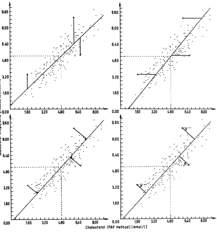
In figure 2 these 4 different structural relationship .lines and the directions of the distance measure are plotted into the scattergram of serum cholesterol measurements obtained by 2 different methods. The experimental data are taken from I.e. (25).

The estimates of the first and second order moments were calculated from these 165 pairs of measurements.

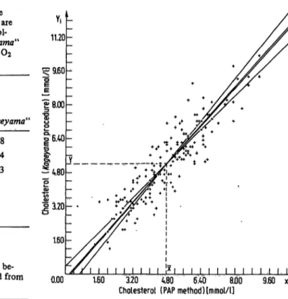
They are summarized in table 2. table 3 shows the corresponding estimates b0 and bt for the intercept and the slope to the x-axis and the estimates lx and ly for the residual standard deviations derived under the different constraints. The scattergram of the observed points and the 4 structural relationship lines are shown in figure 3.

As was pointed out before, all the lines are enclosed by the 2 regression lines. Since the correlation coefficient is near to 1 (0.893), the various structural relationship lines do not differ very much.

The sampling distribution of the slope estimate bt is not known arid even approximative values for the Variance are complicated to derive. An approach to asymptotic

(9)

Feldmann, Schneider» Klinkers t and Haeckel: Multhrariate comparison of analytical methods 129

9.60 -

1.60 120 4BO 6.40 8.00

9.60

È.ÏÏ

6.40

4.80

3.20

1.60

i l Ë l 1 É É É ß l l l l l l l ( l l l l l

0.00 1.60 320 4.80 6.40 8,00

1.60 -

áïï

^{1.60 3.20} 6.40 8.00 0.00 1.60 3.20 4.80 6AO 8.00

Cholesterol (PAP method) tmmol/l]

Fig. 2. The linear structural relationship with 4 different types of constraints a) regression from y to ÷: ë÷ = Ï (È = ~)

c) principle component: ë÷ = Xy (È = 1)

The bars show the direction of distances to be minimized.

b) regression from ÷ to y: \y = Ï (È = 0)

÷² ÷²

ë÷ ^ Ay

d) standardized principle component: — = — (È

expressions for the variances was given by Barnett (12), the following approximative expression for the variance using the fact that the estimates of the structural rela- (with an additive error proportional to (1/n) ' ):

tionship parameters are functions of the sample moments ^

S*, S£ and Sxy = r · Sx · Sy. For such functions approxi- sj^ = — b?(l - r*y).

mative expressions for the variance are known (see I.e.

(8) and appendix 1). Using these expressions we get, for The details of the derivation of this formula and ap- the estimate bj = ± Sy/sx in the standardized principal proximative expressions for the slope under other con- component model (which is most important in practice), straints are given in appendix 1.

J. C!in. Chem. Clin. Biochem. / Vol. 19, 1981 / No. 3

(10)

130 Feldmann, Schneider, Klinkers t and Haeekel: Multivariate comparison of analytical methods Tab. 2. Sample statistics for two methods determining the

cholesterol concentration. The experimental data are taken from I.e. (14). Both methods use cholesterol- oxidase, "PAP'* the Trinder reaction and „Kageyama"

the catalase coupled Hantzsch reaction for the 02 2 detection.

Sample statistics Methods for determining the cholesterol concentration [mmol/lj

X = „PAP" Õ = „Kageyama"

Means Variances

Standard deviations Covariance Correlation No. of samples

x = 4.799 s^x = 2.625 s^x =1.620 s

y = 5.198 s£ = 3.324 sy =1.823

x y= 2.638 r = 0.893 n = 165

Tab. 3. The estimated linear relationship Y* = b0 + fy X* be- tween X = „PAP" and Y = „Kageyama" calculated from table 1 with the sample statistics of table 2.

Statistical analysis

Regression to ÷ Regression to y Principle component Standardized principle component

Intercept

bo 0.377 - 0.849 -0.278 - 0.201

Slope

bi 1.005 1.260 1.141 1.125

Standard deviation of random error 1÷

0.000 0.731 0.560 0.530

V 0.824 0.000 0.560 0.596

In regression analysis (considering regression to the x- axis), it is usually stated that the slope bt is normally distributed with mean value ft and standard deviation

apt = óâ/ãÓ(×ß - x)2, where ae is the standard deviation of the residuals. (In the notation used in this paper we called it Xy). It should be noticed that this statement is true for small values of n, only if the values Xi are considered as fixed and not as realizations of random variables (as in the structural relationship model). So this distributional property of bt in the regression model is conditional on the values xj. Therefore the confidence intervals and tests derived under this distributional property are also conditional on the given xj-values.

Similar results hold for the regression slope b^ to,the y-axis, where the values yj are considered as fixed.

Of the possible hypotheses to be tested, the hypothesis ft = 1 is the most important-one. It states that both measurement methods have the same expected values, what can be interpreted as lack of proportional errors in both measurement methods. It should be noted, that this hypothesis is an additional constraint. As the structural relationship parameters are uniquely related to the second order moments by the constraint ë²/ë^÷ = È², the

I I I I I I I I I. L 0.00 1.60 120 4,80 6 AD 8J3Q

Cholesterol (PAP method)[mmol/l] 9.60 Fig. 3. The different types of linear structural relationship applied

to the same data points as shown in figure 1.

hypothesis ft = 1 imposes a constraint to the second order moments, which may be written as:

4 = È2ó2+ó÷óãñ÷ ã(1-È2) (for ft «1).

In the case of the principal component and standardized principal component model (which are identical for ft = 1 = È) this constraint reduces to:

ó2=ó÷.

So we see that for both these models the hypothesis ft = 1 is equivalent to the hypothesis ay = of (where X and Y are dependent).

A test for this hypothesis was given by Morgan (30). This test is based on a linear transformation of the measurements Xj, yi to Ui, vj according to:

These transformed measurements are realizations of random variables U, V normally distributed with the parameters:

= + = -1 1

); ó2 ^(ó\ +ó\ -2axy)

Puv -

3,

J. Clin. Cherh. Clin. Biochem. / Vol. 19,1981 / No. 3

(11)

Feldmann, Schneider, Klinkersf and Haeckel: Multivariate comparison of analytical methods 131

where ì^÷, ì^÷ , ó\ , ó² and p^xy are the parameters of the bivariate normal distribution of the measurement pairs From these relations it is obvious that the hypothesis

ó÷^{= a}y *^s equivalent to the hypothesis p^uv = 0. This hypothesis can be tested using the sample correlation coefficient r^uv, i.e.

s² -s²

Sx - S y

*xy

According to a well known result (first derived by G sset writing under the pseudonym "Student" in 1908; see I.e. (8), chapter 29.7) the sample statistic

is distributed as Student's t-statistic with n - 2 degrees of freedom under the null hypothesis puv = 0.

Using this result for the case of the principal component and standardized principal component model the hypothesis HQ:/?! = 1 can be tested by the statistic:

This test can be immediately extended to test general simple null hypotheses of the form H0: ^ = 010, where

|3¹⁰ is any given value.

To test this hypothesis we rescale the x^rvalues to 5q = 010 xi (the yj values remain unchanged). If H0 is correct, the structural relationship line between y{ and 5q has the slope 0! = 1. So we have reduced the general null hypothesis j3a = |310 to the specific one: fa = 1 and can apply the test derived above.

It should be noticed that rescaling the Xj changes the variances and constraint È. The error variances of the variables Xj and y^{ have the constraint È² = ë²/ë| = È2/0éï· If the original measurements follow the standardized principal component model with the constraint (under H⁰) È² = 0²⁰, the rescaled measurements Xj, y^{ follow the principal component model with the constraint È2 = 1. For this model the hypothesis fa = j310

is equivalent to the hypothesis J3^t = 1.

The test of the general simple null hypothesis H⁰ :â¹ = j310 uses as test statistic:

which is t-distributed under H⁰ with ç - 2 degrees of freedom.

With a two-sided alternative hypothesis (Ht: fa Ø1) the null hypothesis H0 is to be rejected with an error prob- ability a (e.g. a = 0.05), if the absolute value Itl exceeds the (1 - —)-quantile of the t-distribution. These quantiles are for various degrees of freedom tabulated in nearly all statistical text books.

Applying this test to the two methods for serum cholesterol concentration (25) we get from table 2:

s²= 2.625; $ = 3.324', s^{x y}= 2.638; r^xy = 0.798;

ç = 165.

From these estimates follows:

-0.699^ _

"T655"³·³⁶·

With ç = 2 = 163 degrees of freedom the 0.9995-quantile of the t-distribution (which corresponds to a two-sided error probability á = 0.001) is 3.35. As the absolute value of the calculated t ;(i.e. 3.36} exceeds this level, the null hypothesis ^ = 1 can be rejected with an error probability of less than 0.1 %. the slope of the structural relationship line is very significantly different from 1, which indicates a proportional error of both measurements.

This statistic is t-distributed under H0 with ç - 2 degrees of freedom. If I t(j310)l > tp, where Ñ = 1 - á/2 and tp is the P-quantile of the t-distribution with ç - 2 degrees of freedom, the hypothesis H⁰ is to reject with a two-sided error probability of a.

In this general test the statistic t is a function of the slope fa assumed in the null hypothesis. Fixing the quantile tp we can use this function to calculate confidence bounds for fa to the given confidence probability P, as these bounds are defined by the equation:

= ±

This is quadratic equation in fa. The solutions of this equation are

The first sign corresponds to the sign of/?^t which equals the sign of the correlation coefficient r^xy. The second sign gives the upper and lower confidence limits. This confidence interval is consistent, i.e. for increasing n both confidence limits converge to the parameter |3º, i.e.

the true slope of the structural relationship line in the standardized principal component model. By rearranging the terms in the brackets, we can write for this confidence interval:

J. Clin. Chem. Clin. Biochem. /.Vol. 19,1981 / No. 3

(12)

132 Feldmann, Schneider, Klinkers t and Haeckel: Multivariate comparison of analytical methods where b-j = ± — is the estimate for the slope j8Sy t, B

sx

(B = b^Vl + (1 - r£^y) - 1)) is the bias,

is the (asymptotic) standard deviation of bt and tp, the P-quantile of the t-distribution with n - 2 degrees of freedom.

For the example of the two cholesterol measurements we get (see tab. 2 and 3):

^ =1.125; si = 2.625; s£ =3.324; r£y = 0.798;

n = 165.

Assuming P = 0.95 we find t^p = 1.975 we get:

upper confidence bound: ]3lu= 1.206 lower confidence bound: ^\ = 1 .050.

As the confidence interval does not cover the value 1 , we conclude that the slope |3¹ is significantly different from 1 (as shown by the t-test).

3. Extension to the comparison of more than two methods

3.1 Extension of the structural relationship model

The model of linear structural relationship can immediately be extended to the comparison of more than two analytic methods measuring the value of the same chemical substance (see I.e. (3, 23, 17, 5)). Let us assume that there are m such methods (m > 2). The observed values of method number j in the serum sample number k will be denoted by xjk (j = 1, . . ., m; k = 1, . . :, n).

The Xjk are realizations of random variables Xj, varying between specimens and repeated measurements at the same specimen. As in the case of 2 methods we assume that each random variable Xj can be decomposed in 2 independent random variables Xj and EJ:

where Xj represents the "expected value" and EJ the

"error term" of the method number j.

The expected value reflects the random variation of the analyte between different specimens, if there are no errors in the measurement methods. The error term reflects these measurement errors, which vary randomly within repeated measurements of the same specimen.

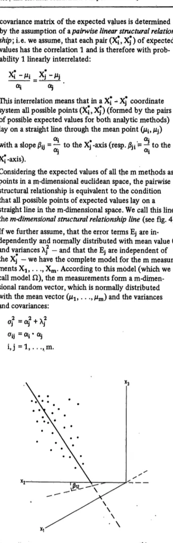
We further assume that the expected values X} ; , . . ., X^

have a m-dimensional, multivariate normal distribution (within the population of all specimens) with the mean vector (ìÀ9 . . ., nm) and the variances (OL\ , . . ., c&). The

covariance matrix of the expected values is determined by the assumption ofupairwise linear structural relation- ship-, i.e. we assume, that each pair (Xj, Xj) of expected values has the correlation 1 and is therefore with probability 1 linearly interrelated:

Oi 05

This interrelation means that in a XJ" - Xj coordinate system all possible points (Xj, Xj ) (formed by the pairs of possible expected values for both analytic methods) lay on a straight line through the mean point (ì^ ì$)

Oj # OL·

with a slope 0y = *- to the Xj -axis (resp. |3ji '= — to the Xi-axis).

Considering the expected values of all the m methods as points in a m-dimensional euclidean space, the pairwise structural relationship is equivalent to the condition that all possible points of expected values lay on a straight line in the m-dimensional space. We call this line the m-dimensional structural relationship line (see fig. 4).

If we further assume, that the error terms EJ are independently and normally distributed with mean value 0 and variances \f — and that the EJ are independent of the Xj - we have the complete model for the m measurements X^1? . . ., X^m. According to this model (which we call model Ù), the m measurements form a m-dimensional random vector, which is normally distributed with the mean vector (ìá, . . ., ìðé) and the variances and cpvariances:

2 2 , ,^2

=

\

Fig. 4. The structural relationship line between 3 measurement values (x-jfc, x²k, *3k) in the 3-dimensional space.

(13)

Feldmann, Schneider, Klinkersf and Haeckel: Multivariate comparison of analytical methods 133 The structural relationship model Ù for m variables

introduces 3 m parameters ì^À9 . . ., /z^m, c%⁹ . . ., c^,,

ëé> · - ·> ëç\, which relate to^{m 2}*^m parameters (i.e.

the means ì-!, . . ,,Mm, the variances o\, . . ., ó^ and covariances o^ (i Ö j)), as shown by the equation above.

The correspondence between the second order moments and the structural parameter 0$ and X² is one-to-one only for the case m = 3. In this case the structural para- meters of and \f can uniquely be calculated by the variances of and covariances ay without any additional constraints:

â- _2 _^ó!2 * <?13 _á_{2 _} _ ^*^ó^!2 á² _ ^{' ^23} ë? «ó? -á?;

ó12

; ë|=ó1-á|.

The pairwise slopes jSjj = Oj/aj, i.e. the slopes to the Xj- axis of the projection of the structural relationship line in the Xj - Xj-plane, are:

_ 3 _ 2 3 _ 3 _ 1 3

P21 oj ó13> Ñ» "è! 'ó*· fe~i-^·

In the case of m > 3 the relations between the second order moments and structural relationship parameters impose constraints to the variances of and covariances QIJ of the variables X1? . . ., Xj. This means that these variables cannot vary unrestricted, but only in such a way that the basic relations remain valid. So by the structural relationship not only the variability of the expected values Xj* but also those of the observed values Xj are restricted if there are more than 3 measurements to compare.

In the case m = 3 the parameters of and Xj* can be estimated by:

1. estimating of and ay (with the usual sample variances Sj2 and covariances Sy) and

2. calculating from these estimates the estimates of 05 and Xj (using the unique one-to-one correspondence).

E.g., estimates of the pairwise slopes y are:

__S23

where the S^u = Ó (x^ik - Xi) (Xjk - Xj) are the (biased) maximum-likelihpQd estimates for the covariances o^.

Approximative values of the sample standard deviations for these estimates can be obtained by using the approxi- mations for functions pf sample-moments, as shown in appendix 1 (see also Barnett (12)).

In the case of m > 3 this estimation procedure is not further applicable, as there is no one-to-one correspondence between 05, Xj and ay. In this case the para-

meters of and X? must be inserted in the likelihood function instead of of and ó^.

This leads to a nonlinear optimization problem, which must be solved numerically. Appropriate computer pro- grams were developed by Feldmann & Klinkers (31).

Also the program package LISREL (23) for general structural relationships can be used.

Tests of hypotheses on the parameters can be performed with the likelihood ratio procedure ofNeyman and Pearson (see e.g. I.e. (30), (24)). According to this proce-

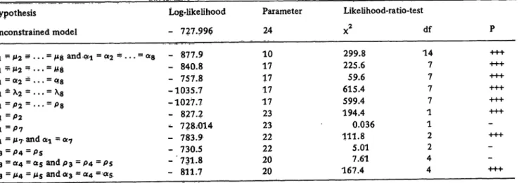
dure the maximum of the log-likelihood function is calculated without and with the constraints imposed by the hypothesis to be tested. If the hypothesis is valid, the twofold difference between the two log-likelihood values L (without the constraint H⁰) and L⁰ (with the constraint HO) is asymptotically x²-distributed with df - df⁰ degrees of freedom (where df is the number of (function- ally) independent parameters under the model Ù and df0 under the constrained model Ù Ð H0).

3.2 Example

The application of the structural relationship methods for the comparison of more than 2 methods will be demonstrated by the following example of which the experimental data are taken from I.e. (25):

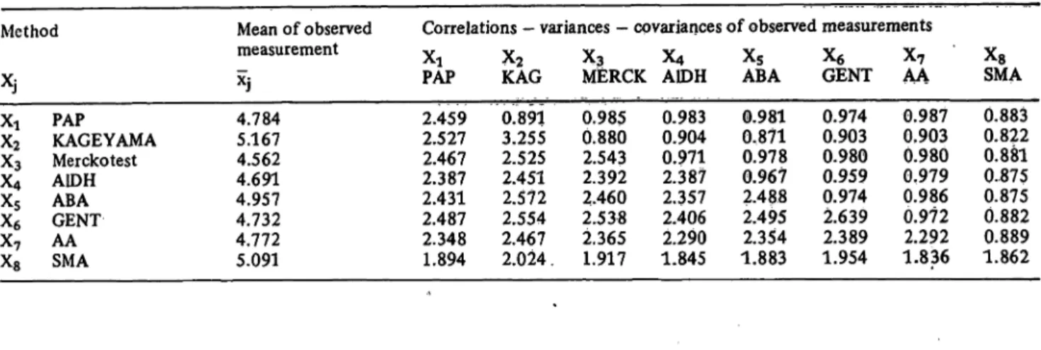
For the determination of the cholesterol concentration in blood serum m = 8 different methods (PAP, Kageyama, Merckotest, A1DH, ABA, GENT, AA and SMA, abbreviations as used in I.e. (25)) were applied to n = 158 sera.

From the results, the mean values ÷], variances Sj², covariances Sy and correlation coefficients ry were calculated (i, j =1, . . ., 8). These estimates are shown in table 4.

To estimate the parameters ì, Oj and Xj the likelihood . function L0 for the unconstrained linear functional

relationship model was maximized, using the program of I.e. (31). The resulting maximum likelihood ML-estimates j, aj and lj are shown in table 5. The log likelihood without constraints is: L = — 728.0. This model implies df = 24 parameters.

As a measure of precision for each method the coefficient of determination R² = a²/s² was calculated (5th column in table 5) and the methods ranked by their precision (6th column in tab. 5). According to this ranking the method PAP has highest precision and the method SMA lowest one. The 8 methods can be con- sidered as equivalent, if their mean values ì-^} and variance components Oj2 are identical. Therefore we test the hypothesis:

and

This hypothesis can be tested by the likelihood ratio test.

J. Clin. Chem. Clin. Biochem. / Vol. 19, 1981 / No. 3

(14)

134 Feidmann, Schneider, Klinkers t and Haeckel: Multivariate comparison of analytical methods Tab. 4. The complete multivariate sample information of m = 8 methods for the determination of cholesterol concentration with

n = 158 samples.

Coefficients of correlation (upper triangle), variances (main diagonal) and covariances (lower triangle).

For abbreviations and experimental data see I.e. (14).

Method

XJ Xi X2

XXs4

X5

X6

X7

Xs

PAP

KAGEYAMA Merckotest A1DH ABA GENT AA SMA

Mean of observed Correlations - variances - covariances of observed measurements

measurement ^ ^ ^ ^ Xg X ÷?

Xj PAP KAG MlERCK A1DH ABA GENT AA 4.784

5.167 4.562 4.691 4.957 4.732 4.772 5.091

2.459 2.527 2.467 2.387 2.431 2.487 2.348 1.894

0.891 3.255 2.525 2.451 2.572 2.554 2.467 2.024 .

0.985 0.880 2.543 2.392 2.460 2.538 2.365 1.917

0.983 0.904 0.971 2.387 2.357 2.406 2.290 1.845

0.981 0.871 0.978 0.967 2.488 2.495 2.354 1.883

0.974 0.903 0.980 0.959 0.974 2.639 2.389 1.954

0.987 0.903 0.980 0.979 0.986 0.972 2.292 1.836

XsSMA 0.883 0.822 0.881 0..875 0.875 0.882 0.889 1.862

Tab. 5. Maximum-likelihood estimates of unconstrained multivariate (m = 8) linear functional relationship. The log-likelihood is LO = - 728.0 with df = 24 parameters.

Method

XJ XtX2

Xs XsX4

XoX7

Xs

PAP

KAGEYAMA Merckotest ADHABA GENTAA SMA

Mean of expected measurement

i*j 4.784 5.167 4.562 4.691 4.957 4.732 4.772 5.091

Standard deviation of expected

measurement

aJ 1.562 1.624 1.577 1.520 1.560 1.594 1.504 1.216

random error lj

0.1685 0.7856 0.2357 0.2756 0.2352 0.3148 0.1723 0.6193

Precision Coefficient of determination Rj^?

0.988 0.810 0.978 0.968 0.078 0.962 0.987 0.794

Rank

17 53 46 28

Tab. 6. Maximum-likelihood estimates of multivariate linear functional relationship under the constraint of both equal expected means and equal expected standard deviations (hypothesis of equal accuracies). The log-likelihood is L0 = - 877.9 with df = 10 parameters.

Method

Xj XiX²

X3

X⁴ XsX6

XTXs

PAP

KAGEYAMA Merckotest A1DHABA GENTAA SMA

Mean of expected measurement

*j 4.773 4.773 4.773 4.773 4.773 4.773 4.773 4.773

Standard deviation of . . expected

measurement

aJ 1.539 1.539 1.539 1.539 1.539 1.539 1.539 1.539