A New Biometrical Procedure for Testing the Equality of Measurements from Two Different Analytical Methods. Application of linear regression procedures for method comparison studies in Clinical Chemistry, Part I

(1)

Passing and Bablok: A new procedure for testing the equality of measurements from two methods 709

J. Clin. Chem. Clin. Biochem.

Vol. 21, 1983, pp. 709-720

A New Biometrical Procedure for Testing the Equality of Measurements from Two Different Analytical Methods

Application of linear regression procedures for method comparison studies in Clinical Chemistry, Part I

By //. Passing

Abt. für Praktische Mathematik, Hoechst AG, Frankfurt/Main 80 and W. Bablok

Allg. Biometrie, Boehringer Mannheim GmbH, Mannheim

(Received December 20, 1982/June 23, 1983)

Summary: Procedures for the statistical evaluation of method comparisons and Instrument tests often have a requirement for distributional properties of the experimental data, but this requirement is frequently not met. In our paper we propose a new linear regression procedure with no special assumptions regarding the distribution of the samples and the measurement errors. The result does not depend on the assignment of the methods (instruments) to X and Y. After testing a linear relationship between X and confidence limits are given for the slope and the intercept a; they are used to determine whether there is only a chance difference between and l and between and 0. The mathematical background is amplified separat- ely in an appendix.

Ein neues biometrisches Verfahren zur Überprüfung der Gleichheit von Meßwerten von zwei analytischen Methoden

Anwendung von linearen Regressionsverfahren bei Methodenvergleichsstudien in der Klinischen Chemie, Teil l Zusammenfassung: Bei der statistischen Auswertung von Methodenvergleichen und bei Geräteerprobungen werden in der Regel Verfahren eingesetzt, deren Anforderungen an die Verteilung der experimentiellen Daten häufig nicht erfüllt sind. In unserer Arbeit schlagen wir daher ein neues lineares Regressionsver- fahren vor, das keine besonderen Annahmen für die Verteilung der Stichprobe und der Meßfehler voraus- setzt. Das Ergebnis ist unabhängig von der Zuordnung der Methoden (Geräte) zu den Variablen X und Y.

Nach Prüfung eines linearen Zusammenhanges zwischen X und Y werden Vertrauensgrenzen für die Stei- gung und den Achsenabschnitt angegeben. Mit ihrer Hilfe werden die Hypothesen = l und = 0 ge- testet. Die mathematischen Grundlagen werden separat in einem Appendix abgehandelt.

Contents 1. Introduction

1. Introduction Parameter estimation in linear regression models is 2. Method Comparison and Linear Regression one of the standard toP^ics >^{n basic} statistical text-

„ . ^^T _ . . books. With the widespread use of pocket calculators 3. A New Regression Procedure the computation of linear regression lines based on 4. Discussion and Examples l^{east S}q^uares has become routine work in scientific 5. Appendix: Mathenaatieal Derivations research. Unfortunately, many textbooks cover the

J. Clin. Chem. CJin. Biochem. / Vol. 21,1983 / No. 11

(2)

710 Passing and Bablok: A new procedurc for testing the cquality of measurements from two mcthods

model assumptions rather briefly and only rarely the reader is warned of the consequences if those assumptions are violated. However, it is in the very nature of many experiments which call for linear regression that most of the assumptions cannot be ob- served. For instance, in many situations there is no independent variable which is free of error; but procedures taking this into account (1,2) are based on more rigid and idealized distributional requirements than can be met in real experiments.

2. Method Comparison and Linear Regression Clinical chemistry is one of the areas where linear regression models play a major role in the statistical evaluation of experiments. Especially in comparing analytical methods for measuring the same chemical substance or in Instrument testing the need for reliable parameter estimation becomes very obvious in the judgement of equality. Clearly a method comparison cannot exclusively be based on the evaluation of a regression model. Many more properties of the methods must be compared; at least accuracy, imprecision, sensitivity, specificity, and r nge of concentration should be studied. For a detailed discussion see I.e. (3,4).

The experimental layout can be described s follows:

There are 2 different methods (Instruments) which measure the same chemical analyte in a given me- dium (e.g. serum, plasma, urine, ...). The question is: Do the methods measure the same concentration of the analyte or is there a systematic difference in the measurements? (For simplicity, we only refer to concentrations but our Statements are also valid for any other quantity.)

The usual experimental procedure is to draw n independent samples from a population in which a given analyte is to the measured with values Xi and yj for the i-th sample. These measurements are realisations of a pair of random variables X and Y, where X represents the values of method l and Υ the values of method 2. For simplicity we also denote method l by method X and method 2 by method Y.

Following the statistical model of I.e. (5) each random variable is the sum of two components:

- ,one variable representing the Variation of the expected value of the analyte within the population of all possible samples;

- one variable representing the Variation of the measurement error for a given sample.

For the i-th sample this relationship is described by the equations

and

xf and yf denote the expected values of this sample• ι

and ξί and ηί give the measurement errofs. In this way each method may have its own expected value for the i-th sample.

If there exists a structural relationship between the two methods it can be described by the linear equation

y t - a + x*

From the n experimental values (Xj,yO the following objectives should be attained:

i) estimation of α and ;

ii) statistical test of the assumption of linearity; and if linearity is given

iii) test of the hypothesis β = 1;

iv) test of the hypothesis α = 0.

If both hypotheses are accepted we can infer y* = xf, i.e. the two methods X and Y measure the same concentration within the investigated concentration r nge.

In practice one of the following four procedures is used:

[1] linear regression yi = α +

[2] linear regression Xj = A + By, + %

[3] principal component analysis (Deming's proced- ure) (5)

[4] standardized principal component analysis (5, 6, 7)

All four procedures assume a linear relation between the two methods, however each one has specific theo^

retical requirements:

— [1] and [2] ask for an error-free independent variable X or Y and normally distributed error terins with constant variance. A statistical test of linearity can be performed only if there exist multiple measurements of the dependent variable¹). Pro- cedures [1] and [2] are not equivalent.and may even give contradictory results.

*) Strictly speaking this test should only be used if the independent variable has fixed values, s is assumed in the usual least squares linear regression.

J. Clin. Chem. Clin. Biocheni / Vol. 21, 1983 / No. <11

(3)

- [3] and [4] assume that the expected values x*

and y* come from a normal distribution. The error terms have to be normally distributed with a constant variance | and o^; they follow the re- strictions

for [3]

and

A statistical test of linearity has not so far been proposed.

However, in method comparison studies we general- ly find the following Situation:

— Neither method X nor method is free of random error.

— The distribution of the measurement errors is usu- ally not normal (8).

— The expected values x* and yf are not a random sample from normal distributions, since the methods are compared over a wide concentration ränge of the analyte which covers values of both healthy and diseased persons.

— Extreme values (outliers) are not necessarily gross measurement errors; they may be caused by different properties of the methods with respect to specificity or susceptibility to interferences. There- fore they should not be removed from the calculation without experimental reason.

— The variance of the measurement errors is not constant over the ränge of concentrations; in fact the variability increases with the magnitude of the measurements.

Therefore it must be expected that a researcher using any of the above procedures may obtain biased estimations for and ß, and therefore misleading results from the experiment. This Situation is equally disappointing for the investigator and the statistician.

In the last 20 yeärs many different proposals have been published forparäineter estimätion in the linear mpdel, using less stringent distributional assumptions.

The estimations were either'based ori robust procedures [for a detailed discussion with references see Lc. (9) and also i.e. (10)] or on a distribution-free approach (11). We are, however, not aware of a pro- posal which deals with the problem of a structural relationship.

We now describe a procedure which can achieve all the objeetives (i) to (iv) and does not require specific assumptions regarding the distributions of the expected values or the error terms.

3. A New Regression Procedure

On the basis of the structural relationship model äs described in chapter 2 we make the following assumptions:

x*,y* are the expected values of random variables from an arbitrary, continuous distribution (i.e.

the sampling distribution is arbitrary).

, are realisations of random error terms, both coming from the same type of distribution.

Their variances | and ojj need not to be constant within the sampling ränge but should re- main proportional, that is

In part II of our paper we shall demonstrate that these rather weak assumptions are sufficient for reliable parameter estimations and hypothesis testing if

— 1. There we shall investigate the influence of the distributions on the result of our procedure.

i) Estimätion of and

According to Theil (12) the slopes of the straight lines between any two points are employed for the estimätion of ß. They are given by

i - Xj for l < i < j < n.

There are (^ ] possible ways to connect any two points. W

Identical pairs of measurements with xⁱ = x^ja n d yⁱ = y^j.

do not contribute to the estimätion of ß; the corresponding Sij is not defined at this stage. For reasons of symmetry (see appendix) any S,j with a value of

— l is also disregarded.

Furthermore, from x^{ = Xj and y^} yj it follows that Sy = ± «>, depending on the sign of the difference y^$ - ^ ; from x^{ Xj and y, = yj it follows that Sy = 0.

Since (X,Y) is a continuous bivariate variable the occurrence of any of these special cases has a probability of zero (experimental data should exhibit these cases very rarely). In total there are

slopes Sjj. After sorting the Sy the ranked sequence

S(l) ^ S(2) < . . . . ^S(N)

is obtained.

J. Clin. Chem. Clin. Biochem. / Vol. 21, 1983 / No. 11

(4)

712 Passing and Bablok: A ncw procedure for testing the cquality of mcasurements from two methods

If we substitute the structural relationship in the de- finition of the S\-^} we find

y t - y t - -

From yf = + ßx* and djj = (x* - x*) we get o ß · djj + ( , - ^)

^ - dij + (6 - ;)

de + d - §) ß

d + Zj

^ dij + Zg '

where Zjj and z§ are indepedent and from the same distribution.

Since the values of Sjj are not independent it is obvious that their median can be a biased estimator of ß. We proceed therefore äs follows:

Let K be the number of values of Sjj with Sjj < -1.

Then using K äs an offset, ß is estimated by the shifted median b of the S(\\:

b =

-y ' (

^S

(T

^+K

)

, if N is odd

if N is even

·

-quan- For the construction of a two-sided confiderice interval for ß on the level let w^ denote the 11 - -^- l-q

2 \ *· l ' tue of the standardized normal distribution.

With

n ( n ~ l)(2n + 5) and 18

(Mi rounded to an integer value) the confidence interval for ß is given by

S(M| + K) < ß < S(M2 + K)·

The introduction of the offset K is motivated by the request for an arbitrary assignment of the methods to X and Y. The definition of K äs the number of values of Sy smaller than -1 correspönds to the null hypothesis ß = 1. It will be demonstrated that, in this case, our b is a good and reliable estimator of ß (see appendix and part II).

The estimation of requires that at least one half of the points is located above or on the regression line and at least one half of the points below or on the line. As (X, Y) is a continuous bivariäte variable then an equal number of points lies above and below the regression line with probability L pöint (x»yi) is located above the line only if a < yi — bx,. Therefofe it can easily be shown that

a = med (y^ — bxi}

is an estimator of a.

If b^L denotes the lower and bu the upper limit of the confidence interval for ß then the corresponding H- mits for are given by

a^L = med {yj - byXj}

a^y == med {y^{ -* b^LXi}.

These limits are conservative.

With the n pairs of measurement (Xi,yj) one can either calculate

y* = a-hbx* or x* = A + By*.

The above estimators for and ß show the following property:

= " - and A = — b '

analogous förmulas hold for their confidence limits.

The proof is given in the appendix. 1t is.therefore irrelevant which one of the two methods is denoted byX.

ii) Statistical fest of the assumption of linearity In testing for linearity one has to inspeet how the regression line fits the data or how randomly the data scatters about y* = a + bx*. Naturally the para- meters a and b are fixed in this context and oür test will be conditional on a and b.

If there is a nonlinear relatioiisMp between x* and y*

one would expect to find too many consecutive measurements either above or below the fitted line. Let l denote the number of points (Xi,yi) with y\ > a + bxi and L the mimber of points with y^ < a-f bxj. To every point (Xi,yj) we assign a score , i.e.

=

and

-y, if y· >

-f-.

^{i f}

yi<

, ifyi =

(5)

Unfortunately the sequence of scores depends on the way in which the points (Xj,yO are ranked: either by increasing X-values or by increasing Y-values. That is, the result of a test for linearity would depend on which one of the methods is assigned to the X- and which one to the Y-variable.

Both methods can be treated alike by sorting the points (Xi,y·,) along the line y* = a-f bx*. This is achieved by projecting every point (Xi,yO on the regression line. The distance between this projection and the y-intercept of the fitted line is given by

Yi+^bl -xj a

Tabl. 1. Critical values of the cusum statistic γ (%) hv

The scores η are sorted according to increasing DJ;

this rank order Γ(ί) becomes the basis of the proposed linearity test.

We have considered two possible Solutions to such a test. An obvious one would be the employment of a run test which actually would test the randomness of the distribution of scores along the line y* = a + bx*.

The test is the subject of many publications [e.g. I.e.

(13)], and its application for testing linearity is dis- cussed in I.e. (14). The other solution which we present is based on a cusum-concept, which is a well known controlling procedure in Clinical Chemistry (15). Consider a coordinate System in which the x- axis represents the ranks of the DJ, i.e. the num- bers l to n, and the y-axis the cumulative sum of the scores τ\. The sum

i

cusum (i) =^k2^jr(k)

denotes the excess of positive or negative scores from point l to point i in the sorted sequence of the DJ . A random arrangement of scores s an in- dication of linearity would result in moderate values of | cusum (i) |, whefeas an excess number of consecutive positive or negative scores in a "large" value of | cusum (i) |. Therefore it seems to be ppropriate to compare the distribution of the subset of η with η > 0 with the distribution of the subset with η < 0.

Critical values for the cusum statistic can be obtained from the Kolmogorov^Smirnov test; the derivation is given in the appendix.

If | cusum (i) | > h^ - VL + 1 holds for some i (i ==

l, ..., n) a nonrand m arrangement of scores can be concluded and^f therefore a linear relationship between x* and y* is rejected (h^Y is tabulated in table 1).

It is obvious that the judgement of linearity depends also on the sampling distribution.

l 105

1.631.36 1.22

iii) Test of the hypothesis β = l

In order to test this hypothesis we make use of the confidence interval for . The hypothesis is accepted if the value of l is enclosed in this interval, otherwise it is rejected. A rejection of β = l demonstrates at least a proportional difference between the two methods. From the theory this test is not independent of the underlying distributions; however, our Simulation study shows that in general it gives reliable results (see appendix and part II).

iv) Test, of the hypothesis α = 0

The hypothesis is accepted if the confidence interval for α contains the value of 0. This is a conservative test. If the hypothesis is rejected both methods differ at least by a constant amount (bias).

If we accept both β = l and α = 0 we can infer y* = x*, or, in other words, both methods are identical.

4. Discussion and Examples

The basic concept of our regression procedure is due to Theil who developed this idea without refer- ence to the problem of method comparison. His paper assumes x,· to be fixed and restricts itself to the estimation of β alone. Our estimation differs slightly from that of Theil, since it employs the offset K, i.e. the number of slopes less than — l, to ascertain the relationship

Consequently, parameter estimation is independent of the assignment of the methods to X and Y.

It is obvious that the estimators a and b are only meaningful if a linear relationship exists between x*

and y*. Otherwise a and b cannot be interpreted.

Clearly the new procedure takes into account the experimental reality of method comparisons s de- scribed in chapter 2.

J, Clin. Chem. Clin. Biochem. / Vol. 21, 1983 / No. 11

(6)

714 Passing and Bablok: A new procedure for testing the eq ality of measurements from two methods

ϋer ί-α»

^3 CD

α»

Ό0

Ο£

Cσ σ_L

£=

0ρ

Όο

JC

"QJ

^L·

CXI

-σο .c-»r (U

χ:

'i«-

•ο0

£2.

Qi

Οc ο :

·—σ α.ε

<— Jο

c \

v χ

X

δ

'X XJ x x

*x X '

x'

X * ' X

δ

1 1 1 1 ll 1 M ι 1 1 1 M 1 ! 1 ll 1 ' 1 MI 1 1 IM 1 M l ':

* ~~

X X

χ χX

v X

X X

χχ Χ X y

X X

χ X y

x v χ

' l l l l l I I I l l l l l l l l l l ( I M I I l l I I l . l l M I l l (O

s

CD C5er

cn

C rv

CD

CD'~

r^·»

CD CD CD CD CD , CD CD

to -»a· cxi cxi ^j· <o

ι ι ι

sanpisay

σo.

Eo o

TDO

EP

•5 —

I

ca.

f

l

c/)

ι

£ ε

Όα>

« g

l

8 II 11

s c ·£

^ ι

'S 2o **-

? 8 I l II _{ε — ***}

•ΌC3

X ^

0 Q

1 2

t l

.'S"o

8.

Co

•o(U

.1

o

c o ^

ο .ε «Ξ

Ιϊ 1

S O a c o ""

€ e

i!

P 1

rt "ce

a l

E « >. 0 « h= JB e Λ Λ

3 00 O 60 W>

« ^ !2 CN m

11

(7)

Passing and Bablok: Λ ncw proccdurc for tcstinp t he «qutility of mcasuremcnts from two inethmU 715

g

XJCM O

CC υ1.

cgc ι

Tc

JC·*-

2c

8

_n

o*

S

5o

5a.

5 3D

S

0

£ C*

^i

«ΌO X.

o*

"o

•~

1 a

E

«»>o X ^

x * *

X K

χ κ X

X

ϊ( v

« X

_{x ^}

X

£*·

*

t i 1

O O O C U3 «N* fxi

sanpi

X ;H

κ_χ x

X X

X

xx

* X X

« K

' » X X

1

W

/

=> S S g sau

δ

c^ir»

g 6c σ»

c3

°^

CDfsi

O

i

l g,

Ou l»

ii

_{B °}

n o l o

OCO

Oo -oo

I

o>

o

8 c

'S "c

11 ii S 8

X ^

ll

||

^ o2 l

sl

Oto

oo

.co o»

s. ff

σ> <

.gco

•g •

8 If

O >,S ii

oiob

J. Clin. Chem. Cfin. Biochem. / Vol. 21, 1983 / No. 11

(8)

716 Passing and Bablok: A new procedure for testing the equality of measurements from two methods

In particular the inconstancy of the variances is the reason for using only signs for the estimation of and the test for linearity. Moreover, all measurement points (Xj,y») have equal weights in the estimation of the regression line; therefore extreme points do not show undue influence on the calculation. The same is true if the ränge of concentration is rather large (i.e. the ränge covers several powers of 10).

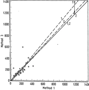
These theoretical arguments are supported by three figures all based on the same set of samples measured by methods l, 2 and 3. In figure l method l is assigned to X and method 2 to Y. In figure 2 this assignment is interchanged. Obviously, all plots within figure 2 are obtained from the corresponding ones in figure l by reflection, showing the independence of the assignment to X and Y. We have chosen this example to demonstrate this property of our procedure even though the estimation of is clearly different from 1.

In figure 3 we cfemonstrate how one extreme point can influence the outcpme of the comparison of method l with method 3. First we calculate our procedure and the standardized principal component with the original data set, i.e. including the extreme point (1180, 1398). The estimations of are 0.998

UOOF

0 200 400 600 800 1000 1200 KOO Method l

Fig. 3. Demonstration of the different behaviour of the new procedure and the standardized principal component when extreme points are present. Further details are given in the text.

New procedure

--- Standardized principal component O Basic data set

O Original point in data set ü Altered point in data set

and 1.165 respectively; the latter is significantly different from 1. We then move the extreme point to the value (1180, 1190) and calculate a second time.

The new results are 0.994 and 1.043, which are both not significant.

It can be argued that this is not ä'fair comparison with a pf ocedure for which the sampling of the data is not adequate. However, the data comes from a real experiment and the standardized principal component analysis is a recommended and often used evaluation procedure (4).

The procedures [1] to [4] are related to each other.

For instance, the slope estimated by procedure [4] is eqüal to the geometric mean of the slope from procedure [1] and the reciprocal of the slope from procedure [2]. Furthermore, the slope of [4] will al·

ways be greater than or equal to that of [1], because b[4] = b[l]/r. Since b[4] is just the ratio of two Standard deviations, it is independent of any jpint function of X and Y. Under the assumption of normal·

ly distributed error terms and expected values the ratio

is estimated by the ratio of the Standard deviations of the measurements. Since the Standard deviation depends only on the sum of the variances of the two Variation components it cannot reflect any independent change in their distributional properties. In con- trast the estimator

b = med \

shows that it can respond to changes in both the sampling and the⁴ error tefm distribution.

Contrary to usual practice, we advise against a State- ment öf the magnitude of dispersion or the coefc ficient of correlation from this experiment. The for- mer adds no further Information tö the result of the regression procedure. The latter is a measure of as- sociation between X and Y and does not describe a functional relationship; besides, it has been shown (16) that its use can lead to erroneous inferences.

Any other properties of the methods must be demonstrated by additional experiments using the ap^

propriate statistics.

The computation of the new procedure appears to foe rather tedious since the slopes Sy inüst be sorted.

This, however, is required by every statistic which calls for ranking. The calculation can easily be car- ried out on any Computer with ät least the size of a mini; several working prograp^s are available at

J. Clin. Chem. Clin. Biochem. / Vol. 21, 1983 / No. H

(9)

Passing and Bablok: A new procedure for tcsting thc equality of measuremcnts from two methods 717 present for various Computers. For small desk Com-

puters with a Standard memory size we have written a PASCAL program which allows the evaluation of up to 70 samples. With sufficient memory this number can easily be extended. This program is available on request. In addition a BASIC program written for a HP 85 desk Computer can be requested; it can easily be adapted to the B ASIC-version of other Computers.

5. Appendix: Mathematical Derivations 7. What does b estimate?

The values for Sjj are identically distributed but not independent. Therefore the sample median of the Sy may give a biased estimation of . It is plausible that a somehow shifted median would be a better estimator. We cannot prove theoretically that the median shifted by our offset K is unbiased. How- ever, we can demonstrate einpirically that our procedure estiinates β correctly in the case of the null hypothesis by using the following Simulation model.

Let [Cu,c0] be the common r nge of concentrations in which both methods are applicable. It is assumed that both methods have constant coefficients of Varia- tion CV^ and Ον^η in [CU,C^Q]. Let

c: = c⁰

The r nge of both methods is transformed into the interval — , l ; in doing so CV^ and CVη re- in unchanged. On — , I n samples are drawn main

with "true values" x? and yf = x? for i = l, ..., n from two different distributions respectively: one in which the x? are equidistant on l—*, l L and one where the samples are skewly distributed over — , l .

L ^ J

The "true values" x* and yf are distorted by inde- pendent "rneasurement errors" §j and r\{ giving

"measured values" Xi = x* + % and yi = y* 4- T|J, Three types of distribution of "measurement errors" are

considered: normal distribution, mixture of two normal distributions, and a skew distribution. c is varied between 2 and oo, n from 40 to 90 and both CV's are varied independently of each other from l % to 13%. The slope b is calculated for every of 500 data sets which are generated for each choice of para- meters and distributions and the median of this 500 slope estimations is computed. The deviation of this median from β = l is an estimate of the bias of b.

From the Simulation we find that b is unbiased for CV's < 7%. The details and the behaviour of our procedure compared with 6 others are given in part II of this paper.

From the above, it follows that a estimates a.

2. The procedure is independent ofthe assignment to X and Υ

For

y* = a + bx* and x* = A + By*

we show that

B = -_D - - .

D

We define

(1)

arctg Sjj

if - l < Sij < oo

(i.e. -45°<arctgS^ij<90°) arctg Sy + 180°

if - oo < Sjj < -1

(i.e. -90° < arctg S^V) < -45°) The domain of ω,-j with -45° < ω^ < 135° lies sym- metrical to 45° which corresponds to the ideal slope of l for a regression line in method comparison.

Since Sy = — l cannot uniquely be assigned to ω^ , we have the choice of including these values in both assignments, or of excluding them — s we have done — from the calculation. If we now interchange X and Y, we find that ω^ is transformed to 90° - (Oij and the rank order of the sorted ω^ is revers- ed, but not changed in the sequence. If the slope conforms to

(2) b = tg med it follows that

B = tg med {90° -

= tg [90° - med tg med {o)ij}

(10)

718 Passing and Bablok: A ncw procedure for testing the equality of mcasurements from two methods

To derive formula (2) let us consider the following two ways of ranking on R \ {—1} u { — » , 00}

which for simplicity's sake are given in graphical form:

I.

II.

-r (- t

^{+ 00}

-i

^-l-oo¹ -l

Ranking according to I gives the natural rank order of the Sy; ranking according to Π shows the corresponding order of the Sjj with Sy = tg-coy, if the <i)jj are ranked ίη the natural order.

Clearly, the sequence in II is the same s in I for the region(-l, + oo]⁵onlythefirstKvalueswithSij < -l are added to the end by a left round-shift. There- fore, if we sort the Sy according to I it is sufficierit to use K s an offset for the deterrnination of the median with respect to rank order II.

b =

if N odd

(rank order I),

= med {Sjj}

= med tg { )ij}

= tg med

if N even

(3) (rank order II)

(natural ranking) (natural ranking) The last equality is exact only for odd N's; however even for N > 40 the difference

will be sufficiently small to justify the equal sign.

The limits of the confidence interval for β can be transformed similarly if X and Υ are interchanged:

S(M,+K) =

= S(M,)

(4) Μ.)

(rank order I) (rank order Π) (rank order II) (rank order Π)

= l (rank order I,

SCN + I-M. + K) X and Y interchanged) The result of testing the hypothesis β = l is therefore independent of the assignment of the methods to X and Y.

'(N + l - M,)

Analogously we obtain for the intercept after interchanging X and Y:

A = med {xj —Byj}

(5) = — med {bxj - b · Byj}l D · r

= —g-med{yi-bXi} = - — .l a

The confidence interval for α can be transformed in the same manner:

AU = med {Xi-BLyi}

τ—DU -b u ' and it follqws that

The result of testing the hypotheses α = 0 is thefe- fore independent f the choice of X.

In the cusum-test the rank order of the O} and of the A femains unchanged if X and Y are interchanged, only the sign of the η is revefsed. Since the test statistic is j cusum (i) | the result is independent of the assignment.

3. J stification of confidence intervals Let

+ * {(i⁵j) | Yi = Yj and xj < Xj) . The last equation in formula (4) is valid if

that is if K(_ «, - 1> < M! holds. Moreover, after interchanging X and Y this condition transforms into K(_ 1>0) < MI. Therefore, the conversion of the limits after interchanging X and Y works if

(6) K(- oo, - D < MI and K(_ Iv0) < MI hold.

To justify the formula for M! and to give a sufficient condition for formula (6) we proceed s follows. In I.e. (17) it is shown that a confidence interval for β can be constructed by determining all those 's for which

Xi and R. = - x

J. Clin. Chem. Clin. Biochem. / Vol. 21» 1983 / No. 11

(11)

Passing and Bablok: A ncw proccdurc for testing the equality of measurcmcnts from two methods 719

are not significantly correlated according to Ken-

daWs . Let

(7)

Q(ß) = * UM) l (Xi-Xj) (Ri-Rj) < 0}

Then P(ß) + Q(ß) = N with probability 1.

From

(xs - Xj) (Ri - Rj) =

(x-,

-

Xj)

2

(Sij

- ß)

follows that

P(ß)

= *

{('O)

l S« > ß}

Therefore the condition

S(M, -t- K) < < S(M2 + K)

is equivalent to

M! + K < Q ( ß ) and M , - K < P ( ß ) and thus to

2M

1

-N<P(ß)-Q(ß)4-2K<N-2M

1

The distribution of C: = P(ß)-Q(ß) does not de- pend on the distribution of (X, Y) whereas the distri- bution of K clearly does so. Therefore, it is impos- sible to derive a formula for MI satisfying

P{S(M,

= P{2M, -N < C + 2K < N-2MJ

= l -a

completely independent of the distribution of (X, Y).

However, C is asymptoticälly normal distributed with E(C)

= 0 and

Therefore it can be concluded that for method com- parisons in clinical chemistry the proposed confid- enee interval for has the actual level of about 95%.

The empirical derivation of this Statement might seem unsatisfactory. But the same Simulation model can also be used to demonstrate the behaviour of the other regression procedures mentioned in chapter 2 under realistic conditions. In our second paper we shall show the favourable properties of our method when compared with the others.

A sufficient condition for (6) is

or

= N - 2 Q ( 0 ) > N - 2 M , = C,;

this is true if X and Y show a significant positive correlation according to Kendall's .

Finally, the actual level of the confidenee interval for is higher than 95%. This is also confirmed from the Simulation model.

4. Test oflinearity — Derivation ofthe cusum statistic

The cusum-test is conditional on a and b; therefore the Dj are conditionally independent. We divide the D,· into two sets, one with scores > 0 and one with

< 0; their empirical distribution function is denot- ed by FI and G L respectively. Then, for

Xe[D(i),D

^(m)

)

we get

such that P{-CY :< C < Cy} = l - holds, with G, defined in chapter 3. Therefore, MI is defmed by

or

M , = ·

We studied the properties of the confidenee interval for on the definition of Mi in the Simulation model and obtajned the following result: If both methods have the same precision then in all cases the actual confidenee level is about 95%; it is never less thän 91% or higher than 96%. More details are given in part II of this paper.

and

F,(X) -

r(k)

r

(k) > 0

VFT * - >

^w

r« < 0

l

VML -'

^r(k)

J. Clin. Chern. CKn. Biochern. / Vol. 21, 1983 / No. 11

(12)

720 Passing and Bablok: A new procedure for testing the equality of measurements from two methods

It follows that

: = sup|F,(X)-GL(X)|

X e R

and

P ( max l cusum (i) l < hX l < i f S n ' V ' ' Y YY · V l + L \ /

with hY beiiig the critical value of the Kolmogorov- Smirnov statistic (18).

References

1. Halperin, M. (1961) J. Amer. Statist. Assoc. 56, 657-669.

2. Madansky, A. (1959) J. Amer. Statist. Assoc. 54, 173-205.

3. Stamm, D. (1979) J. Clin. Chem. Clin. Biochem. 77, 277- 279 and 280-282.

4. Haeckel, R. (1982) J. Clin. Chem. Clin. Biochem. 20, 107- 5. Feldmann, U., Schneider, B., Klinkers, H. & Haeckel, R.110.

(1981) J. Clin. Chem. Clin. Biochem. 79, 121-137.

6. Ricker, W.E. (1973) J. Fish. Res. Board Can. 30, 409-434.

7. Jolicoeur, P. (1975) J. Fish. Res. Board Can. 32,1491-1494.

8. Michotte, Y. (1978) Evaluation of precision and accuracy - comparison of two procedures, In: Evaluation and optimiza- tion of laboratory methods and analytical procedures (Mas- sart, D. L., Dijkstra, A. & Kaufmann, L., eds.), Eisevier, Am- sterdam, Oxford, New York.

9. Heiler, S. (1980) Robuste Schätzung im Linearen Modell, In:

Robuste Verfahren (Nowak, H. & Zentgraf, R., eds.), Sprin- ger Verlag, Berlin.

10. Wolf, G. K. (1980) Praktische Erfahrung mit R-robusten Ver- fahren bei klinischen Versuchen, In: Robuste Verfahren (No- wak, H. & Zentgraf, R., eds.), Springer Verlag, Berlin.

11. Maritz, J.S. (1981) Distribution-Free Statistical Methods, Chapman and Hall, London.

12. Theil, H. (1950) Proc. Kon. Ned. Akad. v. Wetensch, AS 3, Part I 386-392, part II 521-525, part III 1397-1412.

13. Bradley, J. V. (1968) Distribution free Statistical tests. Prent- ice Hall, Englewood Cliffs, N.J.

14. Wold, S. & Sjöström, M. (1978) Lirtear free energy relationship äs tools for investigating chemical similarity — Theory and Practice, In: Correlation Anälysis in Chemistryj Recent Advances (Chapman, N.B. & Shorter, J., eds.), Plenum Press, New York and London.

15. Van Dobben de Bruyn, C.S. (1968) Cumulative Sum Tests:

Theory and Practice, Griffin, London.

16. Cornbleet, P.J. & Shea, M.C, (1978) Clin. Chem. 24, 857- 17. Hollander, M. & Wolfe, D. A. (1973) Nonparametric Statist-861.

ical Methods, J. Wiley & Sons, New York.

18. Witting, H. & Nölle, G. (1970) Angewandte mathematische Statistik, B. G. Teubner. Stuttgart.

Dr. H. Passing

Äbtig, für Praktische Mathematik, Hoechst AG D-.6230 Frankfurt/Main 80

W. Bablok - v

Allg. Biometrie, Boehringer Mannheim GmbH D-6800 Mannheim 3!

J. Clin. Chem. Clin. Biochem.' / Vol. 21, 1983 / No. 11