A test for the parametric form of the variance function in a partial linear regression model

A test for the parametric form of the variance function in a partial linear regression model

Holger Dette

Ruhr-Universit¨at Bochum Fakult¨at f¨ur Mathematik 44780 Bochum, Germany

e-mail: holger.dette@ruhr-uni-bochum.de

Mareen Marchlewski Ruhr-Universit¨at Bochum

Fakult¨at f¨ur Mathematik 44780 Bochum, Germany

email: mareen.marchlewski@ruhr-uni-bochum.de

August 13, 2007

Abstract

We consider the problem of testing for a parametric form of the variance function in a partial linear regression model. A new test is derived, which can detect local alternatives converging to the null hypothesis at a rate n

and is based on a stochastic process of the integrated variance function. We establish weak convergence to a Gaussian process under the null hypothesis, fixed and local alternatives. In the special case of testing for homoscedasticity the limiting process is a scaled Brownian bridge. We also compare the finite sample properties with a test based on an L

-distance, which was recently proposed by You and Chen (2005).

1 Introduction

Partial linear regression models have found considerable interest in the recent literature, because they combine the attractive features of linear models (such as interpretability of the parameter estimates or well established theoretical properties) with the more flexible concept of nonparametric regression [see e.g. Green and Silverman (1994), Yatchew (1997), H¨ardle, Liang and Gao (2000) among many others]. Typically the model is defined as

Y

= x

β + m(t

) + σ(t

)ε

, i = 1, . . . , n, (1.1)

where the Y

are the responses, β = (β

, . . . , β

)

is a vector of unknown parameters and m and

σ are smooth functions. The vectors x

= (x

, . . . , x

) and the real numbers t

(i = 1, . . . , n)

are fixed design points and ε

, . . . , ε

denote random variables with mean 0 and variance 1. Much

effort has been spent on the problem of testing hypotheses regarding β or m [see e.g. Gao (1997),

Fan and Huang (2001), Gonz´alez-Manteiga and Aneiros-P´erez (2003), Aneiros-P´erez, Gonz´alez-

Manteiga and Vieu (2004), Bianco, Boente and Mart´ınez (2006) among many others] but less

literature is available on the problem of testing hypotheses regarding the variance function σ.

In the purely nonparametric model Y

= m(t

) + σ(t

)ε

several authors have emphasized the importance of detecting heteroscedasticity and have proposed various tests for heteroscedasticity [see e.g. Koenker and Basset (1981), Cook and Weisberg (1983), Diblasi and Bowman (1997), Dette and Munk (1998a), Liero (2003) among many others]. Recently, You and Chen (2005) proposed a test for homoscedasticity in the partial linear regression model (1.1), which is based on an estimate of the L

-distance between the variance function σ

(·) and its best constant approximation. This test is - to the knowledge of the authors - the only procedure which has been proposed for testing the hypothesis of homoscedasticity in a partial linear regression model of the form (1.1). It can detect local hypotheses, which converge to the null hypothesis of homoscedasticity at a rate n

, where n denotes the sample size.

The present paper has two purposes. On the one hand we are interested in a test for a homoscedastic error structure which is more efficient with respect to Pitman alternatives, on the other hand we will also consider the more general problem of testing for a parametric form of the variance function, that is

H

: σ

(t) = σ

(t, θ) ∀ t ∈ [0, 1], (1.2)

where σ

(t, θ) is a known function, θ = (θ

, . . . , θ

)

∈ Θ ⊂ R

an unknown vector of parameters and the set Θ is assumed to be compact. Note that the hypothesis of homoscedasticity is obtained for d = 1 and σ

(t, θ) = θ, but many other hypotheses are of interest in practical applications.

In Section 2 we introduce two stochastic processes, which will be used as the basis for constructing test statistics for the hypothesis (1.2). The basic idea is to compare estimates of the integrated variance R

0

σ

(u)du under the null hypothesis and the alternative. Weak convergence of this process to a centered Gaussian process and the corresponding statistical applications are discussed in Section 3. In particular Kolmogorov-Smirnov and Cram´er-von-Mises type tests are proposed and it is demonstrated that the new tests can detect local alternatives converging to the null hypothesis at a rate n

. We also discuss the asymptotic properties of the test in the case of a random design, which differ from the results obtained under the fixed design assumption. In Section 4 we present a small simulation study and compare the new tests with a test which has recently been suggested by You and Chen (2005). We also illustrate the application of the test by means of a data example. Finally, some technical details are given in an Appendix in Section 5.

2 Two new tests for the variance function in partial linear regression models

Recall the definition of the partial linear regression model (1.1). We consider a triangular array of random variables without mentioning this in our notation (that is - we write Y

, t

, x

and ε

instead of Y

, t

, x

and ε

, respectively). For the explanatory variables we consider a fixed design satisfying

i n + 1 =

Z

0

f(t) dt, i = 1, . . . , n, (2.1)

for some positive density f on the interval [0, 1] [see Sacks and Ylvisacker (1970)] and k x

k≤ c, i = 1, . . . , n,

(2.2)

for some constant c ∈ R

(here and throughout this paper k · k denotes the euclidean norm). The case of a random design will briefly be discussed in Section 3.2. If m

(t) = E[ε

] (j = 3, 4) denotes the third and fourth moment of the error (which may depend on t) we further assume

f, σ, m, m

, m

∈ H ol ¨

[0, 1]

(2.3)

for some γ >

, where H ol ¨

[0, 1] denotes the class of all H¨older continuous functions of order γ defined on the interval [0, 1]. The basic idea for the construction of the testing procedure for the hypothesis (1.2) is to eliminate the effect of the linear regression component in the partial linear regression model (1.1) and for this purpose two methods are considered.

The first approach is based on an estimate for the parameter β, which was essentially suggested in a paper by Speckman (1988). This author proposed the estimate

β ˆ

= ( ˆ X

X) ˆ

X ˆ

Y , ˆ (2.4)

where

X ˆ = (I

− K ˆ )X, Y ˆ = (I

− K ˆ )Y,

X = (x

, . . . , x

)

, Y = (Y

, . . . , Y

)

, K ˆ = (W

(t

, h))

,

and W

(t

, h) denote the weights of the local linear estimator at the points t

, that is W

(t

, h) = s ˆ

(t

, h) − s ˆ

(t

, h)(t

− t

)

ˆ

s

(t

, h)ˆ s

(t

, h) − s ˆ

(t

, h) K

µ t

− t

h

¶ , (2.5)

where

ˆ

s

(t

, h) = X

k=1

K

µ t

− t

h

¶

(t

− t

)

,

with a kernel K and a bandwidth h converging to 0 with increasing sample size.

Note that Speckman (1988) considered simpler weights and the homoscedastic partial linear re- gression models, but it can be shown by similar arguments that the statistic ˆ β

is √

n-consistent, if the limit

n→∞

lim 1 n X ˆ

X ˆ (2.6)

exists. We now define modified data by

Y

= Y

− x

β ˆ

, i = 1, . . . , n, (2.7)

and consider the pseudo residuals R

=

X

i=0

d

Y

, j = r + 1, . . . , n,

(2.8)

where (d

, . . . , d

) is a difference sequence satisfying X

i=0

d

= 0, X

i=0

d

= 1 (2.9)

[see Gasser, Sroka and Jennen-Steinmetz (1986) or Hall, Kay and Titterington (1990)]. Note that by the consistency of the estimate ˆ β

and by (2.3) and (2.9) it is intuitively clear that

R

≈ X

i=0

d

(Y

− x

β) = X

i=0

d

m(t

) + X

i=0

d

σ(t

)ε

≈ X

i=0

d

σ(t

)ε

, (2.10)

which implies

E[R

] ≈ X

i=0

d

σ

(t

) ≈ σ

(t

) . (2.11)

Consequently analysis of the variance function can be based on the pseudo residuals R

. For this we define

θ ˆ

= arg min

θ∈Θ

X

i=r+1

³

R

− σ

(t

, θ) ´

(2.12)

as the least squares estimate of the value θ

, which is defined as θ

= arg min

θ∈Θ

Z

0

¡ σ

(t) − σ

(t, θ) ¢

f (t)dt.

(2.13)

Throughout this paper it is assumed that θ

exists, is unique and an interior point of the compact set Θ. We also assume that all partial derivatives up to order three of σ

(t, θ) with respect to the components of θ exist and are continuous in t and θ. We now define for t ∈ [0, 1] the stochastic process

S ˆ

= 1 n − r

X

i=r+1

1

R

− 1 n

X

i=1

1

σ

(t

, θ ˆ

).

(2.14)

It is heuristically clear that ˆ S

is an estimate of the (deterministic) process S

=

Z

0

¡ σ

(u) − σ

(u, θ) ¢

f (u)du , (2.15)

which vanishes (a.e.) for all t ∈ [0, 1] if and only if the null hypothesis (1.2) is valid. Consequently, the hypothesis can be rejected for large values of the Cram´er-von-Mises or Kolmogorov-Smirnov type statistics

C

= n Z

0

| S ˆ

|

F

(dt), K

= √ n sup

t∈[0,1]

| S ˆ

|.

(2.16)

The asymptotic properties of these statistics will be discussed in Section 3.

Our second method for constructing test statistics for the hypothesis (1.2) in the partial linear regression model is based on the observation that

Y ˇ

:= Y

− Y

≈ (x

− x

)β + ˇ ε

, (2.17)

where ˇ ε

= σ(t

)ε

− σ(t

)ε

, and the approximation is motivated by the H¨older continuity of the function m. We introduce the notation ˇ x

= x

− x

(i = 1, . . . , n − 1), ˇ Y = ( ˇ Y

, . . . , Y ˇ

)

, X ˇ = (ˇ x

, . . . , x ˇ

)

, then the estimate

β ˇ

= ( ˇ X

X) ˇ

X ˇ

Y ˇ (2.18)

is √

n consistent, if the limit

n→∞

lim 1 n X ˇ

X ˇ (2.19)

exists and is non-singular. In the same way as in the previous paragraph we now define pseudo residuals as

R

= X

i=0

d

Y

, j = r + 1, . . . , n, (2.20)

where

Y

= Y

− x

β ˇ

, i = 1, . . . , n.

(2.21)

This yields to the alternative stochastic process given by S ˆ

= 1

n − r X

j=r+1

1

R

− 1 n

X

i=1

1

σ

(t

, θ ˆ

), (2.22)

t ∈ [0, 1], where the value ˆ θ

is given by θ ˆ

= arg min

θ∈Θ

X

i=r+1

(R

− σ

(t

, θ))

. (2.23)

Again, by √

n-consistency of the estimate ˇ β

, it is intuitively clear that { S ˆ

}

is a consistent estimate of the stochastic process {S

}

defined in (2.1). The asymptotic properties of the processes { S ˆ

}

and { S ˆ

}

will be investigated in the following section.

3 Asymptotic properties

In this section we present several results on the weak convergence of the stochastic processes

{ S ˆ

}

and { S ˆ

}

in the partial linear regression model and in several extensions of this

model.

3.1 The partial linear regression model with fixed predictors

Our first result specifies the asymptotic properties in the situation described in Section 2. Before we give the precise result, we note that by the assumptions made in Section 2 we have

0 = ∂

∂θ

Z

0

¡ σ

(x) − σ

(x, θ) ¢

f (x)dx

¯ ¯

¯

= −2 Z

0

σ

(x) ¡

σ

(x) − σ

(x, θ

) ¢

f (x)dx, (3.1)

where

σ

(u) = ∂

∂θ

σ

(u, θ)

¯ ¯

¯

, j = 1, . . . , d, (3.2)

denote the partial derivatives of the variance function with respect to the parameters (at the point θ

).

Theorem 3.1. Assume that the assumptions (2.1) - (2.3), (2.6) or (2.19) are satisfied, and define the process { S ˆ

}

either as { S ˆ

}

[see (2.14)] or as { S ˆ

}

[see (2.22)], then the stochastic process { √

n( ˆ S

− S

)}

converges weakly in D[0, 1] to a centered Gaussian process G with covariance kernel

k(t

, t

) = (0, 1)V

Σ

V

(1, 0)

(3.3)

where the matrices Σ

∈ R

and V

∈ R

are defined by

Σ

=



 

 

 



v

v

w

· · · w

v

v

w

· · · w

w

w

z

· · · z

... ... ... ...

w

w

z

· · · z



 

 

 

 , (3.4)

V

= (I

| U), U = −(B

A

, B

A

)

, (3.5)

A = (a

)

, B

= (B

, . . . , B

) (3.6)

and

B

= Z

0

σ

(s)f(s)ds, 1 ≤ i ≤ d a

=

Z

0

σ

(s)σ

(s)f (s)ds, 1 ≤ i, j ≤ d v

=

Z

0

τ

(s)σ

(s)1

(s)f (s)ds, 1 ≤ i, j ≤ 2 w

=

Z

0

τ

(s)σ

(s)σ

(s)1

(s)f(s)ds, 1 ≤ i ≤ 2, 1 ≤ j ≤ d z

=

Z

0

τ

(s)σ

(s)σ

(s)σ

(s)f (s)ds, 1 ≤ i, j ≤ d

τ

(s) = m

(s) − 1 + 4δ

, δ

= X

m=1

Ã

X

j=0

d

d

!

.

We note that the processes ˆ S

and ˆ S

exhibit the same asymptotic behaviour as the corresponding process considered by Dette and Hetzler (2006) in the classical nonparametric regression model.

Consequently, we obtain from Corollary 2.7 in this reference:

Corollary 3.2. Assume that the hypothesis of homoscedasticity H

: σ

(t) = θ

has to be tested (i.e. d = 1, σ

(t) = 1), that the assumptions of Theorem 3.1 are satisfied and that additionally m

(t) ≡ m

is constant. Let { S ˆ

}

denote either the process { S ˆ

}

defined in (2.14) or the process { S ˆ

}

defined in (2.22), then under the null hypothesis of homoscedasticity the process { √

n( ˆ S

− S

)}

converges weakly in D[0, 1] to a scaled Brownian bridge in time F, where F is the distribution function of the design density, i.e.

{ √

n( ˆ S

− S

)}

⇒ q

(m

− 1 + 4δ

)θ

{B ◦ F }

.

Remark 3.3. The test based on the process { √

n( ˆ S

− S

)}

, with ˆ S

either ˆ S

or ˆ S

, can detect alternatives of the form

σ

(t) = σ

(t, θ

) + n

h(t), whenever

h / ∈ span

½ ∂

∂θ

σ

(·, θ)

¯ ¯

¯

, . . . , ∂

∂θ

σ

(·, θ)

¯ ¯

¯

¾ . (3.7)

Here h : [0, 1] → R denotes a fixed function, such that the variance function σ

(t) is nonnegative for all t ∈ [0, 1]. Condition (3.7) results from the weak convergence of the process { √

n( ˆ S

− S

)}

to the process (

G(t) + Z

0

Ã

h(x) − X

j=1

ϕ

∂

∂θ

σ

(x, θ)

¯ ¯

¯

!

f (x)dx )

t∈[0,1]

,

where {G(t)}

denotes the limiting process defined in Theorem 3.1 and the coefficients ϕ

are defined by

(ϕ

, . . . , ϕ

)

= arg min

φ∈R^d

Z

0

Ã

h(x) − X

j=1

φ

∂

∂θ

σ

(x, θ)

¯ ¯

¯

!

f (x)dx.

3.2 Random predictors

As observed in Dette and Munk (1998b) the limit distribution of test statistics for goodness of fit

tests in nonparametric regression models may be different for fixed and random predictors. For

this reason we demonstrate in this subsection the effect of random predictors on the asymptotic

properties of the stochastic processes { S ˆ

}

and { S ˆ

}

. We have to distinguish several cases, corresponding to random and nonrandom x

and t

. We concentrate on the case, where the points t

are random and x

are fixed design points. The other cases are briefly discussed in Remark 3.6.

To be precise we consider the partial linear regression model

Y

= x

β + m(T

) + σ(T

)ε

, i = 1, . . . , n, (3.8)

where x

, . . . , x

are fixed explanatory variables satisfying assumption (2.2) and T

, . . . , T

are i.i.d.

with positive density f on the interval [0, 1]. We denote by m

(t) = E[ε

|T = t] the jth conditional moment of the errors and assume that m

(t) is bounded by some constant, say m

. We consider the processes { S ˆ

}

and { S ˆ

}

defined in Section 2 and 3 where the fixed design points t

have been replaced by the random variables T

, and T

≤ . . . ≤ T

denotes the order statistic of T

, . . . , T

. The pseudo residuals are defined by

R ˆ

= X

i=0

d

Y ˆ

, j = r + 1, . . . , n, (3.9)

with A

, . . . , A

denoting the antiranks of T

, . . . , T

and ˆ Y

is either Y

or Y

corresponding to the two cases considered in Section 2.

The following result shows that in the case of the random design the stochastic processes { S ˆ

}

and { S ˆ

}

have a different asymptotic behaviour. The proof follows from the fact that the random design assumption regarding the explanatory variables T

, . . . , T

does not change the asymptotic properties of the estimates ˆ β

and ˇ β

defined in Section 2. As a consequence the same arguments as given in Section 3.1 show that the asymptotic behaviour of the processes is the same as that of the corresponding processes obtained in the nonparametric regression model Y

= m(T

) + σ(T

)ε

,which was established in Dette und Hetzler (2006).

Theorem 3.4. Consider the partial linear regression model (3.8), assume that the assumptions (2.1) - (2.3), (2.6) or (2.19) are satisfied, and define the process S ˆ

either as S ˆ

or as S ˆ

(with the obvious modification for the random design assumption), then the stochastic process { √

n( ˆ S

− S

)}

converges weakly in D[0, 1] to a centered Gaussian process G with covariance kernel k ¯

= (0, 1)V

Σ ¯

V

(1, 0)

∈ R

, where Σ ¯

= Σ

+ Φ

, the matrix Σ

is given in (3.4),

Φ

=



 

 

 



¯

v

v ¯

w ¯

· · · w ¯

¯

v

v ¯

w ¯

· · · w ¯

¯

w

w ¯

z ¯

· · · z ¯

... ... ... ... ...

¯

w

w ¯

z ¯

· · · z ¯

.



 

 

 

 (3.10)

and the elements of the matrix Φ

are defined by

¯ v

=

Z

0

σ

(s) f (s) ds − Z

0

σ

(s) f (s) ds Z

0

σ

(s) f (s) ds,

(3.11)

¯ w

=

Z

0

σ

(s) σ

(s) f (s) ds − Z

0

σ

(s) f (s) ds Z

0

σ

(s) σ

(s) f (s) ds,

¯ z

=

Z

0

σ

(s) σ

(s) σ

(s) f (s) ds − Z

0

σ

(s) σ

(s) f (s) ds Z

0

σ

(s) σ

(s) f (s) ds.

Note that it follows from Theorem 3.1 and 3.4 that the weak limit of the process { S ˆ

}

is different for the random and fixed design assumption for the explanatory variables t

, which was also observed by Dette and Munk (1998b), who considered an L

-type test for the parametric form of the regression function. However, in the case considered by these authors there is no difference between the two cases in the limit distribution under the null hypothesis. Only under the fixed alternative different distributions are observable. For the processes considered here the limit distributions are even different under the null hypothesis. Consider for example the problem of testing for homoscedasticity H

: σ

(t) = θ

. For the fixed design the limit distribution is specified in Corollary 3.2, while Theorem 3.4 gives the following result for random predictors.

Corollary 3.5. Assume that the hypothesis of homoscedasticity H

: σ

(t) = θ

has to be tested (i.e. d = 1, σ

(t) = 1), that the assumptions of Theorem 3.4. are satisfied and that additionally m

(t) ≡ m

is constant. Let { S ˆ

}

denote either the process { S ˆ

}

defined in (2.14) or the process { S ˆ

}

defined in (2.22) (with the obvious modification for the random design assumption), then under the null hypothesis of homoscedasticity the process { √

n( ˆ S

− S

)}

converges weakly in D[0, 1] to a scaled Brownian bridge in time F, where F is the distribution function of the design density, i.e.

{ √

n( ˆ S

− S

)}

⇒ q

(m

+ 4δ

)θ

{B ◦ F }

.

Remark 3.6. The case of random predictors X

can be considered in a similar manner and it can be shown that the assumption regarding the randomness of the parametric part has no effect on the asymptotic distribution of the stochastic processes { S ˆ

}

and { S ˆ

}

. More precisely consider the model

Y

= X

β + m(T

) + σ(T

)ε

, i = 1, . . . , n,

where T

, . . . , T

are i.i.d. with positive density f on the interval [0, 1] and X

, . . . , X

are i.i.d with density g having compact support such that the analogs of (2.6) and (2.19) hold in probability. In this case Theorem 3.4 remains valid without any changes. Similarly, if the X

are random variables but the T

are fixed design points satisfying (2.1) the corresponding stochastic processes exhibit exactly the same asymptotic behaviour as described in Theorem 3.1.

4 Finite sample properties

In this section we investigate the finite sample properties of two Cram´er-von-Mises tests derived

from the two stochastic processes {S

}

and {S

}

and perform a comparison with the

test based on the L

-distance, which has recently been proposed by You and Chen (2005). We

also analyse a data example to illustrate the application of the new procedure.

4.1 Testing the hypothesis of homoscedasticity

We first concentrate on the problem of testing for homoscedasticity, where it follows from Corollary 3.2 and the continuous mapping theorem that under the null hypothesis H

: σ

(t) = θ

(for some θ

∈ R

) the Cram´er-von-Mises statistic converges weakly, i.e.

C ˆ

= n Z

0

S ˆ

dF

(t) −→

τ

θ

Z

0

B

(F (t))dF (t) = (m

− 1 + 4δ

)θ

Z

0

B

(t)dt,

where ˆ C

is either the statistic ˆ C

or ˆ C

corresponding to the cases ˆ S

= ˆ S

or ˆ S

= ˆ S

, respectively. Consequently the hypothesis of homoscedasticity is rejected if

C ˆ

≥ ω

( ˆ m

− 1 + 4δ

)ˆ θ

.

Here ω

is the (1 − α) quantile of the distribution of the random variable R

0

B

(t)dt and ˆ θ is either ˆ θ

or ˆ θ

corresponding to the least squares estimate

θ ˆ = arg min

θ∈Θ

X

i=r+1

³ R ˆ

− σ

(t

, θ)

´

obtained from the pseudo residuals ˆ R

= R

or ˆ R

= R

, respectively. The estimate ˆ m

for the fourth moment depends on the used difference sequence and in order to reduce the bias we used r = 2 and the sequence

d

= d

= 1/ √

6, d

= −2/ √ 6 (4.1)

[see Gasser et al. (1986) or Dette, Munk and Wagner (1998)]. For this sequence a consistent estimate of m

is given by

ˆ m

=

à 1 18(n − 2)

X

j=3

R ˆ

− 3 1 36(n − 5)

X

k=3

R ˆ

R ˆ

! Ã 1 6(n − 2)

X

j=3

R ˆ

!

, (4.2)

which can be proved by similar arguments as in Dette and Munk (1998a).

The design considered in our study is a uniform design on the interval [0, 1] given by t

= (i−0.5)/n, i = 1, . . . , n and two models are investigated. The first model is given by

Y

= 3.5x

+ cos(2πt

) + σ(t

)ε

with x

= 5t

+ 0.5η

, (4.3)

while the second model is defined by

Y

= x

+ t

/(t

+ 1) + σ(t

)ε

with x

= t

(1 − t

)

+ √ 0.1η

, (4.4)

where in all models the random variable η

are i.i.d. ∼ U(− √ 3, √

3) and the errors ε

are also i.i.d.

∼ U (− √ 3, √

3). For the variance function three cases are considered, namely (I) σ(t) = σ exp(ct)

(II) σ(t) = σ [1 + c sin(10t)]

(4.5)

(III) σ(t) = σ (1 + ct)

where the choice c = 0 always corresponds to the null hypothesis of homoscedasticity and σ = 0.5 [see Dette and Munk (1998a)]. For the calculation of the statistics ˆ C

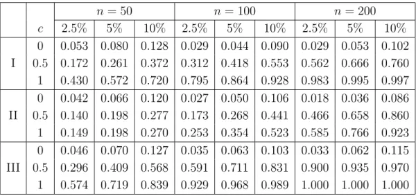
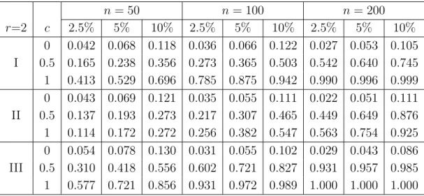
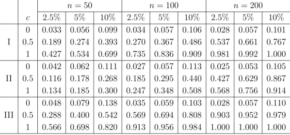
we use Speckman’s (1988) estimate with local linear weights, which requires the specification of a bandwidth and a kernel K. For the latter we used the Epanechnikov kernel, while the bandwidth was chosen according to the rule of Fan and Gijbels (1995). In Table 4.1 and 4.2 we display the corresponding rejection probabilities for sample size n = 50, 100 and 200 based on 1000 simulation runs. The corresponding results for the Cram´er-von-Mises test obtained from the process { S ˆ

}

are presented in Table 4.3 and 4.4 corresponding to example (4.3) and (4.4), respectively. A comparison of the tests based on ˆ C

and ˆ C

shows that there are only minor differences between the two tests. For sample size n = 50 the test based on the statistic ˆ C

yields to a better approximation of the nominal level, while usually the test based on the statistic ˆ C

yields slightly larger rejection probabilities under the alternative.

The results are also directly comparable with simulated rejection probabilities in You and Chen (2005) [see Table 1 and 2 in this reference]. We observe that for the variance functions (I) and (III) in (4.5) the new tests yield substantially larger rejection probabilities. However, for the variance function (II) the test proposed by You and Chen (2005) is more powerful. Note that on a first glance this contradicts asymptotic theory because the test of You and Chen can only detect local alternatives converging to the null hypothesis at a rate n

, while the rate for the new procedures is n

. The reason for the difference between the asymptotic theory and the empirical results for small sample sizes in model (II) can be explained by the specific form of the function S

= R

0

(σ

(x) − θ

)dx = R

0

σ

(x)dx − t R

0

σ

(x)dx which has a maximal absolute value of 0.0924102 in the case c = 0.5 and 0.283507 in the case c = 1. Therefore it is difficult to distinguish these functions from the line ¯ S

≡ 0 and the asymptotic advantages of the new tests will only become visible for very large sample sizes. For example, in model (4.4) with variance structure (II) and n = 1500 observations the rejection probabilities of the test based on the statistic ˆ C

for c = 0.1 are 0.525, 0.750 and 0.918, while they are 0.441, 0.532 and 0.647 for the test proposed by You and Chen (2005), which reflect the asymptotic superiority of the new procedure with respect to Pitman alternatives.

4.2 Bootstrap and testing for a parametric hypothesis

The purpose of this paragraph is twofold. First we explain how the bootstrap can be used in order to improve the finite sample properties of the test procedure. Secondly we investigate the performance of the new procedure for testing for the parametric form of the variance function.

For the sake of brevity we restrict ourselves to the process { S ˆ

}

. For the application of the bootstrap we calculated the residuals

ˆ

ε

= (Y

− x

β ˆ

− m(t ˆ

)) ˆ

σ(t

) , i = 1, . . . , n.

(4.6)

Here ˆ β

is the estimate of Speckman (1988) (with local linear weights) and ˆ m(t) and ˆ σ

(t) are nonparametric estimates of the variance function defined by

ˆ m(t

) =

X

j=1

W

(t

, h)(Y

− x

β ˆ

),

n = 50 n = 100 n = 200

c 2.5% 5% 10% 2.5% 5% 10% 2.5% 5% 10%

0 0.053 0.080 0.128 0.029 0.044 0.090 0.029 0.053 0.102 I 0.5 0.172 0.261 0.372 0.312 0.418 0.553 0.562 0.666 0.760 1 0.430 0.572 0.720 0.795 0.864 0.928 0.983 0.995 0.997 0 0.042 0.066 0.120 0.027 0.050 0.106 0.018 0.036 0.086 II 0.5 0.140 0.198 0.277 0.173 0.268 0.441 0.466 0.658 0.860 1 0.149 0.198 0.270 0.253 0.354 0.523 0.585 0.766 0.923 0 0.046 0.070 0.127 0.035 0.063 0.103 0.033 0.062 0.115 III 0.5 0.296 0.409 0.568 0.591 0.711 0.831 0.900 0.935 0.970 1 0.574 0.719 0.839 0.929 0.968 0.989 1.000 1.000 1.000

Table 4.1: Rejection probabilities of the test (4.1) with C ˆ

= ˆ C

in model (4.3) with a difference sequence of order r = 2. The null hypothesis of homoscedasticity corresponds to the case c = 0.

ˆ

σ

(t

) = X

j=1

W

(t

, h)(Y

− x

β ˆ

− m(t ˆ

))

,

where the weights W

(t

, h) are given in (2.5). The bandwidth h has again been chosen according to the rule of Fan and Gijbels (1995). If ˆ F

denotes the empirical distribution function of the residuals ˆ ε

we generated i.i.d. data ˜ ε

, . . . , ε ˜

∼ F ˆ

and the bootstrap sample

Y ˜

= ˆ m(t

) + σ(t

, θ ˆ

)˜ ε

, i = 1, . . . , n.

where ˆ θ

is defined in (2.12). Finally, the corresponding Cram´er-von-Mises statistic, say ˆ C

, is calculated from the bootstrap data. If B bootstrap replications have been performed and C ˜

< . . . < C ˜

denote the order statistics of the calculated bootstrap sample, the null hypothesis is rejected if

C ˆ

> C ˜

. (4.7)

B = 100 bootstrap replications were performed to calculate the rejection probabilities and 1000 simulation runs were used for each scenario. In Table 4.5 we display the rejection probabilities of this bootstrap procedure for the problem of testing for homoscedasticity in model (4.3). The results are comparable with Table 4.1. It is remarkable that by the bootstrap procedure the approximation of the nominal level is improved substantially, even for sample size n = 50. Moreover, for the variance function (II) the bootstrap procedure yields distinctly larger rejection probabilities under the alternative. A comparison with the results of You and Chen (2005) shows that the bootstrap version of the new tests performs better than the test based on the L

-distance in nearly all cases.

Only for the variance functions (II) the test of You and Chen (2005) yields a substantially larger power, provided that the sample size is small.

Finally, we consider the problem of testing a nonlinear parametric structure for the variance func- tion, that is

H

: σ

(t) = exp(θt) ,

(4.8)

n = 50 n = 100 n = 200

r=2 c 2.5% 5% 10% 2.5% 5% 10% 2.5% 5% 10%

0 0.042 0.068 0.118 0.036 0.066 0.122 0.027 0.053 0.105 I 0.5 0.165 0.238 0.356 0.273 0.365 0.503 0.542 0.640 0.745 1 0.413 0.529 0.696 0.785 0.875 0.942 0.990 0.996 0.999 0 0.043 0.069 0.121 0.035 0.055 0.111 0.022 0.051 0.111 II 0.5 0.137 0.193 0.273 0.217 0.307 0.465 0.449 0.649 0.876 1 0.114 0.172 0.272 0.256 0.382 0.547 0.563 0.754 0.925 0 0.054 0.078 0.130 0.031 0.055 0.102 0.029 0.043 0.086 III 0.5 0.310 0.418 0.556 0.602 0.721 0.827 0.931 0.957 0.985 1 0.577 0.721 0.856 0.931 0.972 0.989 1.000 1.000 1.000

Table 4.2: Rejection probabilities of the test (4.1) with C ˆ

= ˆ C

in model (4.4) with a difference sequence of order r = 2. The null hypothesis of homoscedasticity corresponds to the case c = 0.

n = 50 n = 100 n = 200

c 2.5% 5% 10% 2.5% 5% 10% 2.5% 5% 10%

0 0.036 0.066 0.123 0.025 0.042 0.093 0.026 0.051 0.092 I 0.5 0.169 0.245 0.349 0.285 0.284 0.508 0.558 0.675 0.773 1 0.421 0.531 0.686 0.783 0.862 0.932 0.985 0.992 0.999 0 0.036 0.063 0.108 0.024 0.049 0.094 0.036 0.061 0.117 II 0.5 0.108 0.151 0.249 0.191 0.285 0.448 0.429 0.628 0.850 1 0.124 0.183 0.282 0.245 0.345 0.541 0.540 0.726 0.907 0 0.036 0.060 0.111 0.024 0.057 0.116 0.031 0.055 0.101 III 0.5 0.292 0.409 0.548 0.599 0.718 0.829 0.905 0.958 0.977 1 0.558 0.724 0.845 0.936 0.972 0.986 0.999 1.000 1.000

Table 4.3: Rejection probabilities of the test (4.1) with C ˆ

= ˆ C

in model (4.3) with a difference

sequence of order r = 2. The null hypothesis of homoscedasticity corresponds to the case c = 0.

n = 50 n = 100 n = 200

c 2.5% 5% 10% 2.5% 5% 10% 2.5% 5% 10%

0 0.033 0.056 0.099 0.034 0.057 0.106 0.028 0.057 0.101 I 0.5 0.189 0.274 0.393 0.270 0.367 0.486 0.537 0.661 0.767 1 0.427 0.534 0.699 0.735 0.836 0.909 0.981 0.992 1.000 0 0.042 0.062 0.111 0.027 0.057 0.113 0.025 0.053 0.105 II 0.5 0.116 0.178 0.268 0.185 0.295 0.440 0.427 0.629 0.867 1 0.134 0.185 0.300 0.247 0.348 0.508 0.568 0.756 0.914 0 0.048 0.079 0.138 0.035 0.059 0.103 0.028 0.057 0.110 III 0.5 0.288 0.400 0.542 0.569 0.694 0.808 0.903 0.952 0.979 1 0.566 0.698 0.820 0.913 0.956 0.984 1.000 1.000 1.000

Table 4.4: Rejection probabilities of the test (4.1) with C ˆ

= ˆ C

in model (4.4) with a difference sequence of order r = 2. The null hypothesis of homoscedasticity corresponds to the case c = 0.

n = 50 n = 100 n = 200

c 2.5% 5% 10% 2.5% 5% 10% 2.5% 5% 10%

0 0.024 0.054 0.106 0.020 0.044 0.103 0.017 0.045 0.094 I 0.5 0.158 0.269 0.376 0.287 0.414 0.545 0.574 0.699 0.812 1 0.512 0.667 0.780 0.812 0.901 0.957 0.994 0.997 1.000 0 0.021 0.057 0.121 0.028 0.053 0.098 0.019 0.055 0.114 II 0.5 0.214 0.324 0.491 0.456 0.655 0.863 0.926 0.994 0.999 1 0.364 0.529 0.731 0.820 0.957 0.993 0.998 1.000 1.000 0 0.017 0.048 0.111 0.021 0.052 0.105 0.030 0.069 0.123 III 0.5 0.353 0.535 0.653 0.633 0.757 0.852 0.920 0.959 0.980 1 0.709 0.819 0.904 0.963 0.989 0.996 1.000 1.000 1.000

Table 4.5: Rejection probabilities of the bootstrap test (4.7) with C ˆ

= ˆ C

in model (4.3) with a

difference sequence of order r = 2. The null hypothesis of homoscedasticity corresponds to the case

c = 0.

where the regression model is given by (4.3) and

σ

(t) = (1 + c sin(2πt)) exp(t), (4.9)

with the case c = 0 corresponding to the null hypothesis. The errors ε

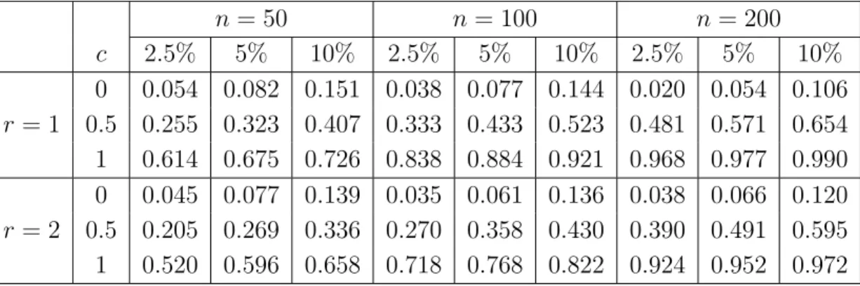
are standard normal distributed and the design is uniform. The corresponding rejection probabilities of the bootstrap test are depicted in Table 4.6 for a difference sequence of order r = 1 and the second order sequence defined in (4.1). In most cases we observe a reasonable approximation of the nominal level for sample sizes larger than 100 and alternatives are detected with rather large power.

n = 50 n = 100 n = 200

c 2.5% 5% 10% 2.5% 5% 10% 2.5% 5% 10%

0 0.054 0.082 0.151 0.038 0.077 0.144 0.020 0.054 0.106 r = 1 0.5 0.255 0.323 0.407 0.333 0.433 0.523 0.481 0.571 0.654 1 0.614 0.675 0.726 0.838 0.884 0.921 0.968 0.977 0.990 0 0.045 0.077 0.139 0.035 0.061 0.136 0.038 0.066 0.120 r = 2 0.5 0.205 0.269 0.336 0.270 0.358 0.430 0.390 0.491 0.595 1 0.520 0.596 0.658 0.718 0.768 0.822 0.924 0.952 0.972

Table 4.6: Rejection probabilities of the bootstrap test (4.7) in model (4.3) with a nonlinear variance function of the form (4.9) and two difference sequences. The null hypothesis (4.8) corresponds to the case c = 0.

4.3 Data example

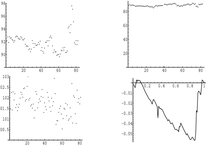
Daniel and Wood (1999) and Bianco et al. (2006) studied a data set of 82 observations obtained in a process variable study of a refinery unit. The response variable Y , which is depicted in the upper left panel of Figure 4.1, is the octane number of the final product. The first three covariates represent the feed compositions and the fourth the logarithm of a combination of process conditions.

For this data we have performed the test for the hypothesis of homoscedasticity, i.e. H

: σ

(t) = θ,

where we have used Speckman’s estimate (1988) with local linear weights to estimate the parameter

β, which is defined in (2.4). We have used the Epanechnikov kernel with bandwidth h = 0.1, which

was chosen according to the rule of Fan and Gijbels (1995). Daniel and Wood (1999) and Bianco

et al. (2006) both discussed the presence of three observations (75 − 77), which extend the range

of the variables Y and x

. The data is depicted in the upper left panel of Figure 4.1. While the

proposed test for homoscedasticity is robust against these three outliers we found that observation

39 has a strong influence on the result of the test. This observation corresponds to an outlier

in the data {Y

− x

β ˆ

}

and yields to a very large pseudo residual. Therefore we did not use

this point in our data analysis. The corresponding plots of the residuals with and without the

39th observation are given in the upper right and lower left panel of Figure 4.1, while the process

{ S ˆ

}

is shown in the lower right panel. The resulting value of the Cram´er-von-Mises statistic

C ˆ

is 0.0877812, which yields to a p-value of 0.065. Therefore the test rejects the hypothesis of

homoscedasticity at level 0.1.

20 40 60 80 90

92 94 96 98

20 40 60 80

20 40 60 80

20 40 60 80

100.5 101 101.5 102 102.5 103

0.2 0.4 0.6 0.8 1

-0.05 -0.04 -0.03 -0.02 -0.01

Figure 4.1: The refinery data discussed in Daniel and Wood (1999) and Bianco et al. (2006) (left upper panel), the residuals {Y

− x

β ˆ

}

(right upper panel). The left lower panel shows the corresponding residuals after deleting the 39th observation and the right lower panel the empirical process { S ˆ

}

based on this data.

5 Appendix

5.1 Proof of Theorem 3.1.

The proof of the theorem has to be given separately for the two processes {S

}

and { S ˆ

}

considered in the theorem.

(a) Weak convergence of { √

n( ˆ S

− S

)}

Recall the definition of the first term ˆ B

:=

P

i=r+1

1

R

in (2.14). At the end of this proof we will show the approximation

D

:= ˆ B

− B ˜

= 1 n − r

X

i=r+1

1

(R

− L

) = o

(n

),

(5.1)

where

B ˜

= 1 n − r

X

i=r+1

1

L

, (5.2)

L

= X

i=0

d

σ(t

)ε

, j = r + 1, . . . , n.

(5.3)

This result and a Taylor expansion now yield S ˆ

= 1

n − r X

i=r+1

1

µ

H

− ∂

∂θ σ

(t

, θ)

¯ ¯

¯

(ˆ θ

− θ

)

¶

+ o

( 1

√ n ) , where the random variables H

are defined by

H

= Ã X

i=0

d

σ(t

)ε

!

− σ

(t

, θ

), j = r + 1, . . . , n.

(5.4)

The H¨older continuity of the function σ therefore implies

√ n( ˆ S

− S

) =

√ n n − r

X

i=r+1

1

à Z

−

X

j=1

σ

(t

)ϑ

!

+ o

(1) , (5.5)

where the random variables Z

are defined by Z

= H

− E[H

] and ϑ

denotes the jth component of the vector ˆ θ

− θ

. Recall the definition (3.2) and define Σ = (σ

(t

))

∈ R

, then it follows from standard results about nonlinear regression [see Seber and Wild (1989), p. 572-574]

that

θ ˆ

− θ

= (Σ

Σ)

Σ

R

− θ

+ O

( 1

n ) = (Σ

Σ)

Σ

H + O

( 1 n

), (5.6)

where R

= ((R

)

, . . . , (R

)

)

, H = (H

, . . . , H

)

and we use the fact that θ

corresponds to the best approximation of the function σ

(·) by functions of the form σ

(·, θ); θ ∈ Θ. Observing (3.1) and the definition of the matrix Σ it therefore follows that

1

n Σ

Σ − A ˆ = O(n

), 1

n Σ

H − 1 n

à X

i=r+1

σ

(t

) (H

− E[H

])

!

j=1

= O

(n

), where

A ˆ = (ˆ a

)

, a ˆ

= 1 n

X

k=1

σ

(t

)σ

(t

).