Asymptotic Normality of Parametric Part in Partial Linear Heteroscedastic Regression Models

ASYMPTOTICNORMALITYOF

PARAMETRICPARTINPARTIAL

LINEARHETEROSCEDASTIC

REGRESSIONMODELS

HuaLiangandWolfgangHardle

AbstractConsiderthepartiallinearheteroscedasticmodelYi=X Ti

+g(Ti)+iei1i nwithrandomvariables(XiTi)andresponsevariablesYiandunknownregressionfunctiong().Weassumethattheerrorsareheteroscedastic,i.e., 2i6=const:eiarei.i.d.randomerrorwithmeanzeroandvariance1.Inthispartiallinearheteroscedasticmodel,weconsiderthesituationsthatthevariancesareanunknownsmoothfunctionofexogenousvariables,orofnonlinearvariablesTi,orofthemeanresponseX Ti

+g(Ti):Undergeneralassumptions,weconstructanestimatoroftheregressionparametervectorwhichisasymptoticallyequivalenttotheweightedleastsquaresestimatoreswithknownvariance.Inprocedureofconstructingtheestimators,thetechniqueofsplittingthesamplesisadopted.

Key W ords and Phrases:

Nonparametricestimation,partiallinearmodel,heteroscedas-tic,semiparametricmodel,asymptoticnormality.

Short title:

Heteroscedasticity

INTRODUCTIONConsiderthesemiparametricpartiallinearregressionmodel,whichisdenedbyYi=X Ti+g(Ti)+"ii=1:::n(1)HuaLiangisAssociateProfessorofStatistics,atInstituteofSystemsScience,ChineseAcademyofSciences,Beijing100080.WolfgangHardleisProfessorofEconometrics,attheInstitutfurStatistikundOkonometrie,Humboldt-UniversitatzuBerlin,D-10178Berlin,Germany.ThisresearchwassupportedbySonderforschungsbereich373\QuantikationundSimulationOkonomischerProzesse".TherstauthorwassupportedbyAlexandervonHumboldtFoundation.TheauthorswouldliketothankDr.UlrikeGrasshoforhervaluablecomments.1

withXi=(xi1:::xip) TandTi201]randomdesignpoints,=(

1:::p) Ttheun-knownparametervectorandganunknownLipschitzcontinuousfunctionfrom01]toIR.Therandomerrors"

1:::"naremeanzerovariableswithvariance1.ThismodelwasstudiedbyEngle,etal.(1986)undertheassumptionofconstanterrorvariance.Morerecentworkinthissemiparametriccontextdealtwiththeestimationofataroot-nrate.Chen(1988),Heckman(1986),Robinson(1988)andSpeckman(1988)constructed pn;consistentestimatesofundervariousassumptionsonthefunctiongandonthedistributionsof"and(XT).Cuzick(1992a)constructedecientestimatesofwhentheerrordensityisknown.TheproblemwasextendedlatertothecaseofunknownerrordistributionbyCuzick(1992b)andSchick(1993).Schick(1996a,b)consideredtheproblemofheteroscedasticity,i.e.,ofnonconstanterrorvariance,formodel(1).Heconstructedroot-nconsistentweightedleastsquaresestimateswithrandomweightofthenite-dimensionalparameter,andgaveanoptimalweightfunctionwhenthevarianceisknownuptoamultiplicativeconstant.HismodelfornonconstantvariancefunctionofYgiven(XT)assumedthatitissomeunknownsmoothfunctionofanexogenousrandomvectorW,whichisunrelatedwithandg.Thepresentpaperfocustouniformlyexistedapproachesintheliteratureandtoextendsomeofexistingresults.Itisconcernedwiththecasesthat 2iissomefunctionofsomeindependentexogenousvariablesforsomefunctionofTiforsomefunctionofX Ti+g(Ti):Theaimofthispaperistopresentauniformlyapplicablemethodforestimatingthepa-rameterontheregressionmodel(1)withheteroscedasticerror,andthentoprovethatinlargesamplesthereisnocostduetoestimatingthevariancefunctionunderappropriateconditions.Inouranalysisitisrelatedtotheliteratureonattentioninsemiparametricmodels.EarlierpapersareBickel(1978),Carroll(1982),CarrollandRuppert(1982)andMuller,etal.(1987).Therearemainlytwokindoftheoreticalanalysis,thatis,theparametricapproach,whichgenerallyassumed 2i=H(Xi)orH(X Ti)forHbeingknown.SeeBoxandHill(1974),Carroll(1982),CarrollandRuppert(1982),JobsonandFuller(1980)andMak(1992)]andthenonparametricapproach,whichassumed 2i=H(Xi)orH(X Ti)forHbeingunknown.SeeCarrollandHardle(1989),FullerandRao(1978)andHallandCarroll(1989)]

2

Letf(YiXiTi)i=1:::ngdenotearandomsamplefromYi=X Ti+g(Ti)+ieii=1:::n(2)whereXiTiTiarethesameastheseinmodel(1).eiarei.i.d.withmean0andvariance1. 2iaresomefunctionsofothervariables,whosespecicformisdiscussedinlatersections.Theclassicapproachworksasfollows.Assumef(XiTiYi)i=1:::n:gsatisfythemodel(2).LetfWni(t)=Wni(tT

1:::Tn)i=1:::ngbeprobabilityweightfunctionsdependingonlyonthedesignpointsT

1:::Tn:Sinceg(Ti)=E(Yi;X Ti).Letbethe"true"value,andthensupposegn(t)= n^X j=1 Wnj(t)(Yj;X Tj) Replacenowg(Ti)bygn(Ti)inmodel(2),wethenobtainleastsquaresestimatorofLS=( f

X

T

f

X

) ;1 f

X

T

f

Y

(3)where f

X

T=( fX

1::: fXn) fXi=Xi; Pnj

=1Wnj(Ti)Xj f

Y

=( eY1::: eYn) T eYi=Yi;nj

=1Wnj(Ti)Yj:Whentheerrorsareheteroscedastic,LSismodiedtoaweightedleastsquaresestimatorW= n^X

i=1 i fXi fX Ti

;1n^X i=1 i fXi eYi (4) forsomeweightii=1:::n.Inourmodel(2)wetakei=1= 2i:Inprincipletheweightsi(or 2i)areunknownandmustbeestimated.Supposefbii=1:::ngbeasequenceofestimatorsof.NaturallyonecantakeWgivenin(4)bysubstitutingbybiasourestimatorof:Inordertodeveloptheasymptotictheory,weusetheideaofsplittingofsample.Letknbetheintegerpartofn=2.b (1)iandb (2)iaretheestimatorsofibasedontherstknsample(X

1T

1Y

1):::(Xk

nTk

nYk

n)andthelatern;knsamples(Xk

n+1Tk

n+1Yk

n+1),:::(XnTnYn)respectively.DenenW= n^X

i=1 bi fXi fX Ti

;1kn Xi=1 b (2)i fXi eYi+ n^X

i=k

n+1 b (1)i fXi eYi (5) astheestimatorof:Thenextstepistoestablishourconclusion,thatis,toprovethatnWisasymptoticnormal.WeintendtoproveWisasymptoticnormal,andthenprove pn(nW;W)3

convergestozeroinprobability.Somenotationsareintroduced."=("

1:::"n) Te"=(e"

1:::e"n) Te"i="i; Pnj

=1Wnj(Ti)"jgni=g(Ti); Pnk

=1Wnk(Ti)g(Tk) bG=(g(T

1)

bgn(T

1):::g(Tn);bgn(Tn)) Thj(t)=E(xijjTi=t),uij=xij;hj(Ti)fori=1:::nandj=1:::p.Wewillusethefollowingassumptions.

Assumption 1.

sup

0t1E(kX

1k 3

jT=t)<1andlimn!11=n Pni

=1iuiu Ti=BandBisapositivedenitematrix.Whereui=(ui1:::uip) T:

Assumption 2.

g()andhj()areallLipschitzcontinuousoforder1.

Assumption 3.

WeightfunctionsWni()satisfythefollowing:(i)max

1in n^X

j=1 Wni(Tj)=O(1)a:s:(ii)max

1ijn Wni(Tj)=O(bn)a:s:bn=n ;2=3(iii)max

1in n^X

j=1 Wnj(Ti)I(jTj;Tij>cn)=O(cn)a:s:cn=n ;1=2log ;1n:

Assumption 4.

ThereexistconstantsC

1andC

2suchthat0<C

1minin imaxin i<C

2:Wesupposethattheestimatorsbiofisatisfysup

1in jbi;ij=oP(n ;q)q1=4(6)WeshallconstructsuchasestimatorsforseveralkindsofiinSections3-5.Thefollowingtheoremspresentgeneralresultsforparameterestimateofpartiallinearheteroscedasticmodels.

Theorem 1.

UnderAssumptions1-4.Wisanasymptoticallynormalestimatorofi.e.,

pn(W;);! LN(0B ;1B

1B ;1)

withB

1=CovfX

1;E(X

1jT

1)g:

Theorem 2.

UnderAssumptions1-4and(6).nWisanasymptoticallyequivalent,i.e.,

pn(nW;)and pn(W;)havethesameasymptoticallynormaldistributions.

Remark. 1.1.

Inthecaseofconstanterrorvariance,i.e. 2i 2,Theorem1wasobtainedbymanyauthors.Seeforexample,Speckman(1988)andGaoetal.(1995).Thepointisthatithasnocostneitherfromtheadaptitionnorthesplittingmethod.4

Remark. 1.2.

Assumptions1-4arerathergeneralinnature,wewillgiveconcreteexamplesinsection3-5.

Remark. 1.3.

Theorem2notonlyassuresthatourestimatorgivenin(5)isasymptoticallyequivalenttotheweightedLSestimatorwithknownweightsbutalsogeneralizetheearlierresultsofrelatedliterature.Theoutlineofthepaperisasfollows.Section2statessomeprelimaryresultsforprovingthemainresults.Sections3-5presentvariousdierentvariancefunctionsandstatethecorrespondingestimates.Section6givesresultsofsimulations.TheproofsofTheorems1and2arepostponedinSection7.

SOMELEMMASInthissectionwemakesomepreparationforprovingourmainresults.Lemma2.1providestheboundednessforhj(Ti); Pnk

=1Wnk(Ti)hj(Tk)andg(Ti); Pnk

=1Wnk(Ti)g(Tk).Itsproofisimmediate.Denotehns(Ti)=hs(Ti); Pnk

=1Wnk(Ti)xks,recallthatuij=xij;hj(Ti)andui=(ui1:::uip) T.Thevariablesfuigarealsoindependentidenticallydistributedrandomvectors.

Lemma 2.1.

SupposethatAssumptions2and3(iii)hold.Then

max

1in Gj(Ti); n^X

k=1 Wnk(Ti)Gj(Tk) =O(cn)forj=0:::p

whereG

0()=g()andGl()=hl()forl=1:::p:

Lemma 2.2.

SupposeAssumptions1-3hold.Thenlimn!1 1n n^X

i=1 i fX Ti

fXi=B

Pro of.

Itfollowsfromxis=hs(Ti)+uisthatthe(sm);thelementof 1n Pni⁼¹i fX Ti

fXi(sm=1:::p)is1n n^X i=1 iexisexim= 1n n^X

i=1 iuisuim+ 1n n^X

i=1 i hns(Ti)uim

+ 1

n n^X

i=1 i hnm(Ti)uis+ 1n n^X

i=1 i hns(Ti) h_nm

(Ti)

def= 1n n^X

i=1 iuisuim+ 1n 3

Xq=1 R (q)nsm

5

Assumption1implieslimn!1i Pni

=1 1n uiu Ti=B:Lemma2.1andAssumption4implyR (3)nsm=o(n):ThenCauchy-SchwarzinequalityyieldsR (1)nsm=oP(n)andR (2)nsm=oP(n):Theseargumentsprovethelemma.NextweshallprovearathergeneralresultonstronguniformconvergenceofweightedaveragesinLemma2.3,whichisappliedinthelaterproofsrepeatly.Firstwegiveanexponentialinequlityforboundedindependentrandomvariables,thatis

Beinstein's Inequalit y.

LetV

1:::Vnbeindependentrandomvariableswithzeromeansandboundedranges:jVijM:Thenforeach>0P(j n^X i=1 Vij>)2exp h

; 2 .n2 n^X i=1 varVi+M oi:

Lemma 2.3.

LetV

1:::Vnbeindependentrandomvariableswithmeanszeroandnitevariances,i.e.,sup

1jnEjVjj r

C<1(r2):Assume(akiki=1:::n)beasequenceofpositivenumberssuchthatsup

1iknjakijn ;p1forsome0<p

1<1and Pnj

=1aji=O(n p2)forp

2max(02=r;p

1):Thenmax

1in n^X

k=1 akiVk =O(n ;slogn)fors=(p1;p2)=2:a:s:

Pro of.

DenoteV 0j=VjI(jVjjn 1=r)andV 00j=Vj;V 0jforj=1:::n:LetM=Cn ;p1n =rand=n ;slogn:ByBeinstein'sinequalityP nmax

1in n^X

j=1 aji(V 0j;EV 0j) >C

1 o

n^X

i=1 P n n^X

j=1 aji(V 0j;EV 0j) >C

1 o

2nexp

; C

1n ;2slog 2n2 Pnj

=1a 2jiEV 2j+2n;p1+1=r;slogn 2nexp(;C 2

1Clogn)Cn ;3=2forsomelargeC

1>0:Thelastsecondinequalityfromn

Xj=1 a 2jiEV 2jsupjajij n^X

j=1 ajiEV 2j=n ;p1+p2andn ;p1+1=r;slognn ;p1+p2:ByBorel-CantelliLemmamax

1in n^X

j=1 Wnj(Ti)(V 0j;EV 0j) =O(n ;slogn)a:s:(7)Let1p<2,1=p+1=q=1suchthat1=q<(p

1+p

2)=2;1=r.ByHolder'sinequalitymax

1in n^X

j=1 aji(V 00j;EV 00j) max¹in n^X

j=1 jajij q

1=qn^X j=1 jV 00j;EV 00jj p

1=p

Cn ;(p1q;1)=q n^X

j=1 jV 00j;EV 00jj p

1=p(8)

6

Observethat1n n^X

j=1

jV 00j;EV 00jj p

;EjV 00j;EV 00jj p

!0a:s:(9)

andEjV 00jj p

EjVjj rn ;1+p=r,andthenn

Xj=1 EjV 00j;EV 00jj p

Cn p=ra:s:(10)

Combining(8),(9)with(10),weobtain

max

1in n^X

k=1 aki(V 00k;EV 00k) Cn ;p1+1=q+1=r=o(n ;s)a:s:(11) Lemma2.3followsfrom(7)and(11)directly.Letr=3Vk=ekorukl,aji=Wnj(Ti)p

1= 2

3 andp²=0:Weobtainthefollowingformulas,whichwillplaycriticalrolesintheprocessofprovingthetheorems.maxin n^X k=1 Wnk(Ti)ek =O(n ;1=3logn)a:s:(12)

andmaxin n^X

k=1 Wnk(Ti)ukl =O(n ;1=3logn)forl=1:::pa:s:

VARIANCEISAFUNCTIONOFOTHERRAN-

DOMVARIABLESThissectionisdevotedtothenonparametricheteroscedasticitystructure 2i=H(Wi)HunknownLipschitzcontinuouswherefWii=1:::ngarealsodesignpoints,whichareassumedtobeindependentofeiand(XiTi)anddenedon01].Dene

cHn(w)= n^X

j=1 fWnj(w)(Yj;X TjLS;bgn(Ti)) 2

astheestimatorofH(w).WhereffWnj(t)i=1:::ngisasequenceofweightfunctionssatisfyingalsothesameassumptionsonfWnj(t)j=1:::ng:7

Theorem 3.1.

Underourassumptions,sup

1in j cHn(Wi);H(Wi)j=oP(n ;1=3logn)

Pro of.

Set"i=ieifori=1:::n.Notethat

cHn(Wi)= n^X j=1 fWnj(Wi)(eYj;fX TjLS) 2

= n^X

j=1 fWnj(Wi)f fX Tj(;LS)+eg(Ti)+e"ig 2

=(;LS) T n^X

j=1 fWnj(Wi) fX Tj(;LS)+ n^X

j=1 fWnj(Wi)eg 2(Ti)+ n^X

j=1 fWnj(Wi)e"i

+2(;LS) n^X

j=1 fWnj(Wi) fX Tj

eg(Ti)+2(;LS) n^X j=1 fWnj(Wi) fX Tj

e"i

+2 n^X

j=1 fWnj(Wi)eg(Ti)e"i(13) Since Pnj

=1 fXj fX Tjisasymmetricmatrix,and0< fWnj(Wi)Cn ;2=3,n

Xj=1 f fWnj(Wi);Cn ;2=3

g fXj fX Tj

isappnonpositivematrix.RecallthatLS;=O(n ;1=2).Theseargumentsmeanthersttermof(13)isOP(n ;2=3):Thesecondtermof(13)iseasilyshowntobeorderOP(n 1=3c 2n):Nowwewanttoshowthatsupi n^X

j=1 fWnj(Wi)e" 2i;H(Wi) =OP(n ;1=3logn)(14)Thisisequivalenttoprovethefollowingthreeitemssupi n^X

j=1 fWnj(Wi) nn^X

k=1 Wnk(Tj)"k o

2

=OP(n ;1=3logn)(15)

supi n^X

j=1 fWnj(Wi)" 2i;H(Wi) =OP(n ;1=3logn)(16)

supi n^X

j=1 fWnj(Wi)"j nn^X

k=1 Wnk(Tj)"k o=OP(n ;1=3logn)(17) (12)assuresthat(15)holds.LipschitzcontinuityofH()andassumptionsonfWnj()entails(16),i.e.,supi n^X

j=1 fWnj(Wi)" 2i;H(Wi) =OP(n ;1=3logn)(18)

8

whoseproofissimilarasthatofLemma2.1.Bytakingaki= fWnk(Wi)H(Wk)andVk=e 2k;1andr=2andp1=2=3andp2=0inLemma2.3,wehavesupi n^X

j=1 fWnj(Wi)H(Wj)(e 2j;1) =OP(n ;1=3logn)(19) Acombinationof(19)and(18)means(15).(16)and(15)andCauchy-Schwarzinequalityimply(17).Thusweproved(14).Thelaterthreetermsof(13)arealloforderoP(n ;1=3logn)byCauchy-Schwarzinequalityandtheconclusionsfortherstthreetermsof(13).ThuswecompletetheproofofTheorem3.1.

VARIANCEISAFUNCTIONDESIGNTiInthissectionweconsiderthecaseinwhichwesupposethevariance 2iisafunctionofthedesignpointsTi,i.e. 2i=H(Ti)HunknownLipschitzcontinuousSimilarasinsection3,wedeneourestimatorofH()as

cHn(t)= n^X

j=1 fWnj(t)fYj;X TjLS;bgn(Ti)g 2

Theorem 4.1.

Underourassumptions,sup

1in j cHn(Ti);H(Ti)j=oP(n ;1=3logn)

Pro of.

TheproofofTheorem4.1issimilartothatofThorem3.1andisomitted.

VARIANCEISAFUNCTIONOFTHEMEANHereweconsiderthemodel(2)with 2i=HfX Ti+g(Ti)gHunknownLipschitzcontinuouswhichmeansthatthevarianceisaunknownfunctionofmeanresponse.ArelatedsituationsinlinearandnonlinearmodelsarediscussedbyCarroll(1982),BoxandHill(1974),Bickel

9

(1978),JobsonandFuller(1980)andCarrollandRuppert(1982).Engleetal.(1986),Greenetal.(1985)andWahba(1984)andothersstudiedtheestimatorfortheregessionfunctionX T+g(T).SinceH()isassumedcompletelyunknown,thestandardmethodistogetinformationaboutH()byreplication,i.e.,weconsiderthefollowing"improved"partiallinearhet-eroscedasticmodelYij=X Ti+g(Ti)+ieijj=1:::mii=1:::nHereYijistheresponseofthejthreplicateatthedesignpoint(XiTi),eijarei.i.d.withmean0andvariance1,,g()and(XiTi)arethesameasthatinmodel(2).WewillborrowtheideaofFullerandRao(1978)forlinearheteroscedasticmodeltoconstructanestimateof 2i.Thatis,tocomputepredictedvalueX TiLS+bgn(Ti)bytleastsquaresestimateLSandnonparametricestimatebgn(Ti)tothedata,andresidualsYij;fX TiLS+bgn(Ti)gandestimate

b 2i= 1mi m

i

Xj=1 Yij;fX TiLS+bgn(Ti)g] 2:(20)Wheneachmistaysbounded,FullerandRao(1978)concludedthattheweightedestimatebasedon(20)andtheweightedleastsquaresestimatesbasedonthetrueweightshavedierentlimitingdistributionsresultsfromthefactthatb 2idonotconvergeinprobabilitytothetrue 2i.

Theorem 5.1.

Letmi=ann 2qdef=m(n)forsomesequenceanconvergingtoinnite.Underourassumptions,sup

1in jb 2i;HfX Ti+g(Ti)gj=oP(n ;q)q1=4

Pro of.

Weonlyoutlinetheproofofthetheorem.Infact

jb 2i;HfX Ti+g(Ti)gj3fX Ti(;LS)g 2+3fg(Ti);gn(Ti)g 2+ 3mi m

i

Xj=1 2i(e 2ij;1)ThersttwoitemsareobviouslyoP(n ;q):Sinceeijarei.i.d.withmeanzeroandvariance1,aftertakingmi=ann 2q Pm

ij=1(e 2ij;1)isequivalentto Pm(n)j=1(e 2

1j;1):UsingthelawoftheiteratedlogarithmandtheboundednessofH()oneknowthat1mi m

i

Xj=1 2i(e 2ij;1)=Ofm(n) ;1=2logm(n)g=oP(n ;q)ThuswederivetheproofofTheorem5.1.10

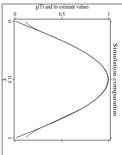
SIMULATIONWepresentasmallsimulationstudytoexplainthebehaviourofthepreviousresults.Wetookthefollowingmodelwithdierentvariancefunctions.Yi=X Ti+g(Ti)+i"ii=1:::n=300Heref"igarestandardnormalrandomvariables,fXigandfTigarebothofuniformrandomvariableson01]:=(10:75) Tandg(t)=sin(t).Thesimulationnumberforeachsituationis500:Threemodelsforthevariancefunctionsareconsidered.LSEandWLSErepresenttheleastsquaresestimatorandtheweightedleastsquaresestimatorgivenin(3)and(5),re-spectively.

Model1: 2i=T 2i

Model2: 2i=W 3iwhereWiarei.i.d.uniformlydistributedrandomvariables.

Model3: 2i=a1expa2fX Ti+g(Ti)g 2]where(a1a

2)=(1=41=3200):ThismodelismentionedbyCarroll(1982)withouttheitemg(Ti).

TABEL 1: Sim ulation results ( 10

;3

)

EstimatorVariance

0=1

1=0:75ModelBiasMSEBiasMSELSE18.6968.729123.4019.1567WLSE14.2302.25921.932.0011LSE212.8827.23125.5958.4213WLSE25.6761.92350.3571.3241LSE35.94.35118.838.521WLSE31.871.7623.942.642Fromtabel1,onecanndthatourestimator(WLSE)isbetterthanLSEinthesenseofbothbiasandMSEforaboveeachmodel.Bytheway,wealsomentionthebehaviouroftheestimatefornonparametricpart,thatisn

Xi=1 ! ni(t)( eYi; fX TinW)

11

Simulation comparation

00.51T

0 0.5 1

g(T) and its estimate values

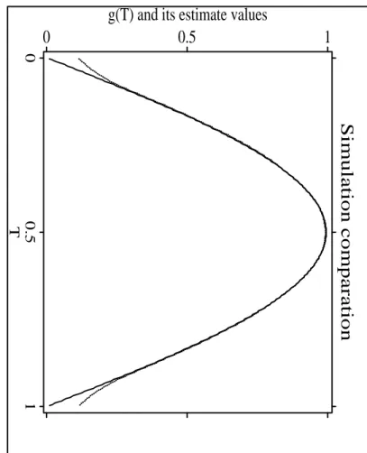
Figure1:Estimatesofthefunctiong(T)fortherstmodel! ni()areotherweightfunctionswhichalsosatisfytheAssumption3.Inprocedureofsimula-tions,wetakeNadaraya-Watsonweightfunctionwithquartickernel(15=16)(1;u 2) 2I(ju1)anduseCross-Validationcriteriontoselectbandwidth.Figures1,2,3aredevotedtothesimulationresultsofthenonparametricpartsforthemodels1,2,3,respectively.Inthefollowinggures,solid-linesforrealvaluesanddished-linesforourestimatevalues.Theguresindicatethatourestimatorsfornonparametricpartperformalsowellexcepttheneighbourhoodsofthepoints0and1.

7PROOFSOFTHEOREMSFirsttwonotationsareintroduced.

bAn= n^X

i=1 bi fXi fX TiAn= n^X

i=1 i fXi fX TiForanymatrixS,s(jl)denotesthe(jl)-thelementofS.

Pro ofo fTheorem 1.

ItfollowsfromthedenitionofWthatW;=A ;1n nn^X i=1 i fXieg(Ti)+ n^X i=1 i fXie"i o

12

Simulation comparation

00.51T

0 0.5 1

g(T) and its estimate values

Figure2:Estimatesofthefunctiong(T)forthesecondmodel

Simulation comparation

00.51T

0 0.5 1

g(T) and its estimate values

Figure3:Estimatesofthefunctiong(T)forthethirdmodel

13

Wewillcompletetheproofbythefollowingthreesteps,forj=1:::p(i)H

1j=1= pn Pni

=1iexijeg(Ti)=oP(1)(ii)H

2j=1= pn Pni

=1iexij n

Pnk

=1Wnk(Ti)ek o=oP(1)(iii)H

3=1= pn Pni

=1i fXiei;! LN(0B ;1B

1B ;1):Theproofof(i)ismainlybasedonlemmas2.1and2.3.Denotehnij=hj(Ti)

Pnk

=1Wnk(Ti)hj(Tk):Note

pnH

1j= n^X

i=1 iuijgni+ n^X

i=1 ihnijgni; n^X

i=1 i n^X

q=1 Wnq(Ti)uqjgni(21) InLemma2.3wetaker=2Vk=ukl,aji=gnj 1

4 <p

1< 1 3 andp2=1;p1:Thenthersttermof(21)isOP(n ; 2p

1;1

2)=oP(n 1=2)Thesecondtermof(21)canbeeasilyshowntobeorderOP(nc 2n)byusingLemma2.1.Thethirdtermof(21)canbehandledbyusingAbel'sinequalityandlemmas2.1and2.3.Hence

n^X

i=1 n^X

q=1 iWnq(Ti)uqjgni C

2nmaxin jgnijmaxin n^X q=1 Wnq(Ti)uqj =O(n 2=3cnlogn):

Thuswecompletetheproofof(i).Wenowshow(ii),i.e., pnH

2j!0:Noticethat

pnH

2j= n^X

i=1 i nn^X

k=1 exkjWni(Tk) oei= n^X

i=1 i nn^X

k=1 ukjWni(Tk) oei+ n^X

i=1 i nn^X

k=1 hnkjWni(Tk) oei

; n^X

i=1 i hn^X

k=1 nn^Xq=1 uqjWnq(Tk) oWni(Tk) iei(22) Theorderofthersttermof(22)isO(n ; 2p

1;1

2logn)bylettingr=2Vk=ek,ali=

Pnk

=1ukjWni(Tk)and 1

4 <p

1< 1 3 andp²=1;p1inLemma2.3.ItfollowsfromLemma2.1and(12)thatthesecondtermof(22)isboundedby

n^X

i=1 i nn^X

k=1 hnkjWni(Tk) oei nmaxkn n^X

i=1 Wni(Tk)ei maxjkn jhnkjj=O(n 2=3cnlogn)a:s:(23)

14

Thesameargumentasthatfor(23)yieldsthatthethridtermof(22)cabbedealtwithas

n^X

i=1 i hn^X

k=1 nn^Xq=1 uqjWnq(Tk) oWni(Tk) iei nmaxkn n^Xi=1 Wni(Tk)ei maxkn k^Xq=1 uqjWnq(Tj) =O(n 13log 2n)=o(n 1=2)a:s:(24)Acombination(22){(24)entails(ii).FinallythecentrallimittheoremandLemma2.2derivethat1

pn n^X

i=1 i fXiei;! LN(0B

1) whichandthefactthatAn!Bimplythat1

pn A

;1n n^X

i=1 i fXiei;! LN(0B ;1B

1B ;1):

ThiscompletestheproofofTheorem1.

Pro ofo fTheorem 2.

InordertocompletetheproofofTheorem2,weprove

pn(nW;W)=oP(1)Firstwestateafact,whoseproofisimmediatelyderivedby(6)andLemma2.2,1n jban(jl);an(jl)j=oP(n ;q)(25)forjl=1:::p.Thiswillbeusedlaterrepeatly.ItfollowsthatnW;W= 12 nA ;1n(An; bAn) bA ;1n n^X i=1 i fXieg(Ti)

+bA ;1n kn

Xi=1 (i;b (2)i)fXieg(Ti)+bA ;1n(An;bAn)bA ;1n n^X

i=1 i fXieei

+ bA ;1n kn

Xi=1 (i;b (2)i) fXieei+ bA ;1n n^X

i=k

n+1 (i;b (1)i) fXieg(Ti)

+bA ;1n n^X

i=k

n+1 (i;b (1)i)fXieei o(26)

ByCauchy-Schwarzinequality,foranyj=1:::p,

n^X

i=1 iexijeg(Ti) C pnmaxin jeg(Ti)j n^X

i=1 ex 2ij

1=2

15

ThisisoP(n 3=4)bylemmas2.1and2.2.Thuseachelementofthersttermof(26)isoP(n ;1=2)bywatchingthefactthateachelementofA ;1n(An; bAn) bA ;1nisn ;5=4.ThesimilarargumentshowsthateachelementofthesecondandfthtermsisalsooP(n ;1=2).RecallthattheproofsforH

2j=oP(1)andH

3convergestonormaldistribution,weconcludethatthethirdtermof(26)isalsooP(n ;1=2).Thusweseethatthedicultproblemistoshowthatthefourthandthelasttermsof(26)arebothoP(n ;1=2).Sincetheirproofsarethesame,weonlyshowthat,forj=1:::p,

n

bA ;1n kn

Xi=1 (i;b (2)i)fXieei oj =oP(n ;1=2)

orequivalentlyk

n

Xi=1 (i;b (2)i)exijeei=oP(n 1=2)(27) Letfngbeasequencenumbersconvergetozerobutsatisfyn>n ;1=4.Thenforany>0andj=1:::p

P nkn

Xi=1 (i;b (2)i)exijeiI(ji;b (2)ijn)>n 1=2 o

P nmaxin ji;b (2)ijn o

!0(28)

Thelaststepisdueto(6).NextweshalldealwiththetermP nkn

Xi=1 (i;b (2)i)exijeiI(ji;b (2)ijn)>n 1=2 o

byChebyshv'sinequality.Sinceb (2)iisindependentofeifori=1:::kn,wecaneasilycalculateE nkn

Xi=1 (i;b (2)i)exijei o

2

Thisiswhyweusesplittingtechniqnetoestimateibyb (2)iandb (1)i.Infact,

P nkn

Xi=1 (i;b (2)i)exijeiI(ji;b (2)ijn)>n 1=2 o Pkni=1Ef(i;b (2)i)I(ji;b (2)ijn)g 2EkfXik 2Ee 2in 2

C k_n

2nn2 !0(29)

16

Thus,by(28)and(29),k

n

Xi=1 (i;b (2)i)exijei=oP(n 1=2)Finally

kn

Xi=1 (i;b (2)i)exij nn^X

k=1 Wnk(Ti)ek o

pn kn

Xi=1 fX 2ij

1=2maxin ji;b (2)ijmaxin n^X

k=1 Wnk(Ti)ek ThisisoP(n 1=2)byusing(25)and(12)andLemma2.2,whichand(29)entail(27).WecompletetheproofofTheorem2.

REFERENCES

Bickel,P.J.(1978).UsingresidualsrobustlyI:Testsforheteroscedasticity,nonlinearity.AnnalsofStatistics,

6

266-291.Bickel,PeterJ.,Klaasen,ChrisA.J.,Ritov,Ya'acovandWellner,JonA.(1993).Ecientandadaptiveestimationforsemiparametricmodels.TheJohnsHopkinsUniversityPress.Box,G.E.P.andHill,W.J.(1974).Correctinginhomogeneityofvariancewithpowertrans-formationweighting.Technometrics

16

,385-389.Carroll,R.J.andHardle,W.(1989).Secondordereectsinsemiparametricweightedleastsquaresregression.Statistics

2

,179-186.Carroll,R.J.(1982).Adaptingforheteroscedasticityinlinearmodels,AnnalsofStatistics,

10

,1224-1233.Carroll,R.J.andRuppert,D.(1982).Robustestimationinheteroscedasticitylinearmodels,AnnalsofStatistics,

10

,429-441.Chen,H.(1988).Convergenceratesforparametriccomponentsinapartlylinearmodel.AnnalsofStatistics,

16

,136-146.Cuzick,J.(1992a).Semiparametricadditiveregression.JournaloftheRoyalStatisticalSociety,SeriesB,

54

,831-843.Cuzick,J.(1992b).Ecientestimatesinsemiparametricadditiveregressionmodelswithunknownerrordistribution.AnnalsofStatistics,

20

,1129-1136.Engle,R.F.,Granger,C.W.J.,Rice,J.andWeiss,A.(1986).Semiparametricestimatesoftherelationbetweenweatherandelectricitysales.JournaloftheAmericanStatisticalAssociation,

81

,310-320.17

Fuller,W.A.andRao,J.N.K.(1978).Estimationforalinearregressionmodelwithunknowndiagonalcovariancematrix.AnnalsofStatistics,

6

,1149-1158.Green,P.,Jennison,C.andSeheult,A.(1985).Analysisofeldexperimentsbyleastsquaressmoothing.JournaloftheRoyalStatisticalSociety,SeriesB,

47

,299-315.Hall,P.andCarroll,R.J.(1989).Variancefunctionestimationinregression:theeectofestimatingthemean.JournaloftheRoyalStatisticalSociety,SeriesB,

51

,3-14.Heckman,N.E.(1986).Splinesmoothinginpartlylinearmodels.JournaloftheRoyalStatisticalSociety,SeriesB,

48

,244-248.Jobson,J.D.andFuller,W.A.(1980).Leastsquaresestimationwhencovariancematrixandparametervectorarefunctionallyrelated.JournaloftheAmericanStatisticalAssocia-tion,

75

,176-181.Mak,T.K.(1992).Estimationofparametersinheteroscedasticlinearmodels.JournaloftheRoyalStatisticalSociety,SeriesB,

54

,648-655.Muller,H.G.andStadtmuller,U.(1987).Estimationofheteroscedasticityinregressionanalysis.AnnalsofStatistics,

15,

610-625.Robinson,P.W.(1987).Asymptoticallyecientestimationinthepresenceofheteroscedas-ticityofunknownform.Econometrica,

55

,875-891.Robinson,P.M.(1988).Root-N-consistentsemiparametricregression.Econometrica,

56

,931-954.Schick,A.(1987).Anoteontheconstructionofasymptoticallylinearestimators.JournalofStatisticalPlanning&Inference,

16

,89-105.Correction

22

,(1989)269-270.Schick,A.(1996a).Weightedleastsquaresestimatesinpartlylinearregressionmodels.Statistics&ProbabilityLetters,

27

,281-287.Schick,A.(1996b).Ecientestimatesinlinearandnonlinearregressionwithheteroscedasticerrors.ToappearbyJournalofStatisticalPlanning&Inference.Speckman,P.(1988).Kernelsmoothinginpartiallinearmodels.JournaloftheRoyalStatisticalSociety,SeriesB,

50

,413-436.Wahba,G.(1984).Partialsplinemodelsforthesemi-parametricestimationofseveralvari-ables.InStatisticalAnalysisofTimeSeries,319-329.

18