Bootstrap Approximations in a Partially Linear Regression Model

PARTIALLY LINEAR REGRESSION

MODEL

Wolfgang Hardle

¹

, Hua Liang

¹²

and Volker Sommerfeld

¹

Institut fur Statistik und Okonometrie

and Sonderforschungsbereich 373 Humboldt-Universitat zu Berlin

D-10178 Berlin, Germany

¹

Institute of Systems Sciences

and

Beijing 100080, China

²

Abstract

Consider the semiparametric regression model ^Yi =^XiT+^g(^Ti)+ⁱ (ⁱ= 1^:::n), where (^XiTi) are known and xed design points, is a ^p;dimensional unknown parameter,^g() is an unknown function on 01]ⁱ are i.i.d. random errors with mean 0 and variance ². In this paper we rst construct bootstrap statisticsⁿ and²ⁿ by resampling. Then we prove that, for the estimatorsⁿandⁿ² of the parameters and

2

p

n(^n;n) and^pn(^n;)^pn(^{n2 ;2n}) and^pn(^n2;2) have the same limit distributions, respectively. The advantage of the bootstrap approximation is explain.

The feasibility of this approach we also show in a simulation study.

Key Words and Phrases:

Semiparametric regression model, bootstrap approximation, asymptotic normality.

AMS 1991 subject classication:

Primary: 62G05 Secondary: 60F15.

This research was supported by Sonderforschungsbereich 373 \Quantikation und Simula- tion Okonomischer Prozesse". The work of Hua Liang was partially supported by Alexander von Humboldt Foundation. The authors are extremely grateful to Dr. Michael Neumann for his many valuable suggestions and comments which greatly improved the presentation of the paper. Corresponding Author: Hua Liang, Institut fur Statistik und Okonometrie, Spandauerstr.1, D-10178 Berlin. Email:hliang@wiwi.hu-berlin.de.

1

Consider the model given by

Yⁱ =X^iT + g(Tⁱ) +ⁱi = 1::: (1) where Xⁱ = (xⁱ¹:::x^ip)^T(p 1) and Tⁱ(T^{i 2} 01]) are known design points, = (¹:::^p)^T is an unknown parameter vector and g is an unknown function, and ¹:::ⁿ are i.i.d. random variables with mean 0 and unknown variance ²:

This model is important because it can be used in applications where one can assume that the responses Yⁱ and predictorsXⁱ is linear dependence, but nonlinearly related to the independent variables Tⁱ. Engle, et al. (1986) studied the eect of weather on electricity demand. Liang, Hardle and Werwatz (1997) used the model to investigate the relationship between income and age from German data. From the point of theory, this model generalizes the standard linear model, by restricts multivariatenonparametric regression which is subject to "Curse of Dimensionality" and is hard to interpret. Therefore, there is a lot of literature studied this model recently. Heckman (1986), Speckman (1988), Chen (1988) considered the asymptotic normality of estimators of and ²: Later Cuzick (1992a, b) and Schick (1993) discussed asymptotic properties and asymptotic eciency for these estimators. Liang and Cheng (1993) discussed the second order asymptotic eciency of LS estimator and MLE of : The technique of bootstrap is a useful tool for the approximation of an unknown prob- ability distribution and therefore for its characteristics like moments or condence regions.

This approximation can be performed by dierent estimators of the true underlying distribu- tion that should be well adapted to the special situation. In this paper we use the empirical distribution function which puts mass of 1=n at each residual in order to approximate the underlying error distribution (for more details see section 2). This classical bootstrap tech- nique was introduced by B. Efron (for a review see e.g. Efron & Tibshirani, 1993). Note that for a hetereoscedastic error structure a wild bootstrap procedure (see e.g. Wu, 1986 or Hardle & Mammen, 1993) would be more appropriate.

Hong and Cheng (1993) considered bootstrap approximation of the estimators for the parameters in the model (1) in the case where ^fXⁱTⁱi = 1:::n^g are i.i.d. random variables andg() is estimated by a kernel smoother. The authors proved that their bootstrap approximation is the same as the classic methods, but failed to explain the advantage of

2

the bootstrap method, which will be discussed in this paper. We will construct bootstrap statistics of and ², and studies their asymptotic normality when (XⁱTⁱ) are known design points and g() is estimated by general nonparametric tting. Analytically as well as numerically we will show that the bootstrap techniques provide a reliable method to approximate the distributions of the estimates.

The eect of smoothing parameter is studied in a simulation study. Thereby it turns out that the estimators of the parametric part are quite robust against the choice of the smoothing parameter. More details can be found in section 3.

The paper is organized as follows. In the following we explain the basic idea for estimating the parameters and give the assumptions on the Xⁱ and Tⁱ. Section 2 constructs bootstrap statistics of and ². In section 3 we present a simulation study in order to complete the asymptotic results. In section 4 some lemmas required later are proven. Section 5 presents the proof of the main result. For the convenience and simplicity, we shall employ C(0 < C <¹) to denote some constant not depending onn but may assume dierent values at each appearance.

Generally there are two methods, backtting and local likelihood ones, to estimate the linear parameter. The asymptotic variance of the two estimates is the same. Here we adopt local likelihood method. Specically, x one estimates g() as a function of to obtain g(), which is a nonparametric estimation problem. Then letting g =b g(), one estimates^b the parametric component, and this is a parametric problem. The detailed discussions can be also found in Severini and Staniswalis (1994).

To estimate g for xed , let !ⁿⁱ(t) = !ⁿⁱ(tT¹:::Tⁿ) be positive weight functions depending only on the design points T¹:::Tⁿ: Assume ^fXⁱ = (xⁱ¹:::x^ip)^TTⁱYⁱi = 1:::n:^g satisfy the model (1). ^g(t) = ^Pnj=1!^nj(t)(Y^{j ;}X^jT) is just the nonparametric estimate of g(t) for xed . Given the estimator ^g(t), an estimate of ⁿ, is obtained basing on Yⁱ =X^iT + ^g(Tⁱ) +ⁱ for i = 1:::n:

Denote ^f

X

= (X^f1:::X^fn)^T X^fi = X^{i ;Pnj=1}!^nj(Tⁱ)X^j

Y

^f = (Y^e1:::Y^en)^T Y^ei = Y^{i ;}

P

n

j=1!^nj(Tⁱ)Y^j: Then the estimate ⁿ can be expressed as ⁿ = (^f

X

^Tf

X

)^;1f

X

^T

Y

^f

In addition, the estimate of ², ⁿ² is naturally dened as ²ⁿ= 1n^Xi=1n (Y^i;X^iTn;gⁿ(Tⁱ))²

3

which is equal to ^1nPni=1(Y^ei;X^fiTn)²: Where gⁿ(t) =^Pnj=1!^nj(t)(Y^j;X^jTn) is the estimate of g(t).

In the following we list the sucient conditions for our main result.

Condition 1.

There exist functions h^j() dened on 01] ^{such that}

x^ij =h^j(Tⁱ) +u^ij 1in 1j p (2) where u^ij is a sequence of real numbers which satisfy lim^{n!1 1nPni=1}uⁱ = 0 and

lim

n!1

n1

n

X

i=1

uⁱu^Ti =B (3)

is a positive denite matrix, and limsup

n!1

a1ⁿ max

1k n

k

X

i=1

uⁱ

<¹ (4)

holds, where uⁱ = (uⁱ¹:::u^ip)^T andaⁿ=n⁵⁼⁶log^;1n:

Condition 2.

g() and h^j() are Lipschitz continuous of order 1.

Condition 3.

The weight functions !ⁿⁱ() satisfy the following:

(i) max

1in n

X

j=1

!^nj(Tⁱ) =O(1) (ii) max

1ijn

!ⁿⁱ(T^j) =O(bⁿ) (iii) max

1in n

X

j=1

!^nj(Tⁱ)I^(jTj;Tij>cn) =O(cⁿ) where bⁿ =n^;2=3 cⁿ=n^;1=3logn:

These conditions are not more complicated than that given in related literature. They are usually needed for establishing asymptotic normality for the estimators of the parameters.

Specically, imposing Condition 1 in that we can lead 1=n^f

X

^Tf

X

converges to B. In fact, (2) of Condition 1 is parallel to the case

h^j(Tⁱ) =E(x^ijjTⁱ) and u^ij =x^{ij ;}E(x^ijjTⁱ)

when (XⁱTⁱ) are random variables. (3) is similar to the result of the strong law of large numbers for random errors. (4) is similar to the law of the iterated logarithm. More detailed discussions may be found in Speckman (1988) and Gao et al. (1995).

The weight functions satised the above condition 3 are presented in Liang, Hardle and Werwatz (1997). Interested readers please nd them there.

4

SULT

The statisticsⁿand ⁿ² have asymptotic standard normal distributions under mild assump- tions. Our simulation studies indicate that the normal approximation does not work very well for small samples. Therefore in this section we propose a bootstrap method as an alternative to the normal asymptotic method.

In the semiparametric regression model the observable columnn^;vector

^

of residuals is given by

^

=

Y

^;

G

^n;

X

^Tn

where

G

ⁿ = ^fgⁿ(T¹):::gⁿ(Tⁿ)^gT. Denote ⁿ = ^{n1 Pni=1}^ⁱ. Let ^Fⁿ be the empirical dis- tribution of

^

, centered at the mean, so ^Fⁿ puts mass 1=n at ^^i;n and ^R xd ^Fⁿ(x) = 0:

Given

Y

, let ¹:::ⁿ be conditional independent with common distribution ^Fⁿ let be the n^;vector whose ith component is ⁱ, and let

Y

=

X

^Tn+

G

ⁿ+ :

Informally,

^

is obtained by resampling the centered residuals. And

Y

is generated from the data, using the regression model with ⁿ as the vector of parameters and ^Fⁿ as the distribution of the disturbance terms .

So we have reason to dene the estimates of and ² as follows, respectively, ⁿ= (^f

X

^Tf

X

)^;1f

X

^Tf

Y

and ²ⁿ = 1n^Xi=1n (Y^{ei ;}X^fiTn)²

where Y^ei =Y^{i ;Pnj=1}!^nj(Tⁱ)Y^j

Y

^f = (Y^e1:::Y^en)^T:

The bootstrap principle is that the distributions of^pn(^n;n) and^pn(^{n2 ;2n}), which can be computed directly from the data, approximate the distributions of ^pn(^n;) and

pn(^{n2 ;2}), respectively. As will be shown later, this approximation is likely to be very good, provided n is large enough. This fact is stated as the following theorem.

Theorem 1.

Suppose conditions 1-3 hold. If E⁴¹ < ^{1 and} max^1inku^ik C⁰ < ¹: Then

sup^xP ^fpn(^n;n)< x^g;P^fpn(^n;) < x^g!0 (5) 5

and

sup^xP ^fpn(^{n2 ;n2})< x^g;P^fpn(^2n;2)< x^g!0 (6) where and below P and E denote the conditional probability and conditional expection given

Y

:

Now, we outline our proof of the theorem. First we decompose^pn(^n;) and ^pn(^{n; n}) into three terms, and ⁿ² and ⁿ² into ve terms, respectively. Then we will calculate the tail probability value of each term. Some additional notations are introduced. = (¹:::ⁿ)^T = (^{e e1}:::^en)^{T ei} = ^{i ;Pnj=1}!^nj(Tⁱ)^j g^ei = g(Tⁱ)^{;Pnk =1}!^nk(Tⁱ)g(T^k)

f

G

= (g^e1:::g^en)^T: We have from the denitions of ⁿ and ⁿ, and ²ⁿ and ⁿ²

pn(^n;) = ^pn(^f

X

^Tf

X

)^;1(^f

X

^Tf

G

+^f

X

^T)^e

= ^pn(^f

X

^Tf

X

)^;1hXn

i=1

Xfⁱg^ei;Xn

i=1

Xf^inXn j=1

!^nj(Tⁱ)^jo+^Xn

i=1

Xfⁱⁱⁱ

def= n(^f

X

^Tf

X

)^;1(H^1;H²+H³):

pn(^n;n) = ^pn(^f

X

^Tf

X

)^;1(^f

X

^T

G

^fn+^f

X

^T )^e

= ^pn(^f

X

^Tf

X

)^;1hXn

i=1

Xf^ieg^ni;Xn

i=1

Xf^inXn j=1

!^nj(Tⁱ)^{j o}+^Xn

i=1

Xf^{ii i}

def= n(^f

X

^T

X

^f)^;1(H^{1 ;}H² +H³):

Where

G

^fn = (g^en1:::g^enn)^T with g^eni =gⁿ(Tⁱ)^{;Pnk =1}!^nk(Tⁱ)gⁿ(T^k) for i = 1:::n:

ⁿ² = 1n

Y

^fTfI^;f

X

(^f

X

^Tf

X

)^;1

X

^fTg

Y

^f

= 1n^T; 1

n^T

X

^f(^f

X

^T

X

^f)^;1f

X

^T _{+ 1n}^f

G

^TfI ^;

X

^f(^f

X

^Tf

X

)^;1f

X

^Tgf

G

;

2n^f

G

^T

X

^f(^f

X

^Tf

X

)^;1f

X

^T _{+ 2n}^f

G

^T

def= I^1;I²+I^3;2I⁴+ 2I⁵: ⁿ² = 1n^f

Y

^TfI^;f

X

(^f

X

^Tf

X

)^;1

X

^fTg

Y

^f

= 1n ^{T ;} 1

n ^Tf

X

(^f

X

^Tf

X

)^;1f

X

^T _{+ 1n}

G

^fnT(I^;f

X

(^f

X

^T

X

^f)^;1f

X

^T)

G

^fn

;

n2

G

^fnTf

X

(^f

X

^Tf

X

)^;1

X

^fT _{+ 2n}^f

G

^nT

def= I^{1 ;}I² +I^{3 ;}2I⁴ + 2I⁵: 6

HereI is the identity matrix of order p. The following sections will prove that H^1jH^2j = o^P(1) and H^1jH^2j = o^P (1) and Iⁱ = o^P(n^;1=2) and Iⁱ = o^P (n^;1=2) for j = 1:::p and i = 2345:

We have up to now showed that the bootstrap method performs as least as well as the normal approximation with the error rate of o^p(1) and o(1), respectively. It is natural to expect that the bootstrap method should perform better than this however. Indeed, our numerical experience means that it is case. In fact, it is also true analytically as is shown in the following theorem.

Theorem 2.

Let M^jn() (²)] and M^jn() (²)] be the j^;th moments of ^pn(^n;) (^pn(^n2;2))] and^pn(^n;n) (^pn(^{n2 ;n2}))], respectively. Then under the conditions 1-3 and E⁶¹ <¹ and max^1inku^ik C⁰ <¹

M^jn()^;M^jn() = O^P(n^;1=3logn) and M^jn(²)^;M^jn(²) =O^P(n^;1=3logn) for j = 1234:

The proof of theorem 2 can be completed by the arguments of Liang (1994) and similar procedures behind. We omit the details.

Theorem 2 indicates that the bootstrap distributions have much better approximation for the rst four moments for ⁿandⁿ² , which are most important quantities in characterizing distributions. Indeed, by Theorem 1 and Lemma 1 given later, one can only obtain that

M^jn()^;M^jn() = o^P(1) andM^jn(²)^;M^jn(²) =O^P(1) for j = 1234 in contrast to Theorem 2.

3 NUMERICAL RESULTS

In this section we present a small simulation study in order to illustrate the nite sample behavior of the estimator. We investigate the model

Yⁱ =Xⁱ + g(Tⁱ) +ⁱ (7)

where g(Tⁱ) =sin(Tⁱ), = (15)⁰ and ⁱ Uniform(^;0:30:3). The independent variables Xⁱ = (Xⁱ⁽¹⁾Xⁱ⁽²⁾) andTⁱare realizations of aUniform(01) distributed random variable. We analyze sample sizes of 3050100 and 300. For nonparametric tting, we use a Nadaraya- Watson kernel weight function with Epanechnikov kernel. We performed the smoothing with

7

sample size n=30

standardized observations

densities

-0.05 0.0 0.05

051015

• • • •• •• •••••

•

•

•

•

•

•

•

•

•

•

•• •• •

•

•

•

•

•

•

•

•

•

•

•

•

••

•• •

• • • • • •

Figure 1

: Plot of of the smoothed bootstrap density (lines), the normal ap- proximation (stars) and the smoothed true density (vertical lines).

dierent bandwidths using some grid search. Thereby it turned out that the results for the parametric part are quite robust against the bandwidth chosen in the nonparametric part.

In the following we present only the simulation results for the parameter ², those fore ¹ are similar.

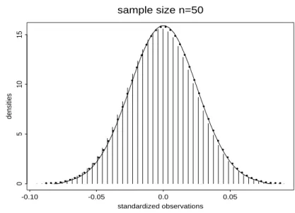
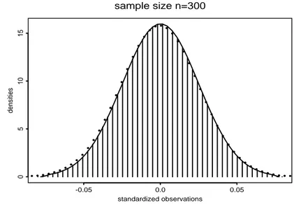
In gures 1 to 4 we plotted the smoothed densities of the estimated true distribution of

pn(^{b2 ;2})= with^{b b2} = ^1nPni=1(~Y^{i ;} ~X^iTn)² for sample sizes 30, 50, 100, 300. Addition- ally we added to these plots the corresponding bootstrap distributions and the asymptotic normal distributions, where we estimated the asymptotic variance ²B^;1 by ^b2B^b;1 with B =b ^{n1 Pni=1} ~X^iT ~Xⁱ and sigma^{b 2} dened above. It turns out that the bootstrap distribution and the asymptotic normal distribution well approximates the true one even for moderate sample sizes of n = 30.

4 SOME LEMMAS

Under the conditions of Theorem 1, Gao et al.(1995) obtained asymptotic normalities of ⁿ and ²ⁿ and convergence rate of gⁿ, which are given in Lemma 1. Lemma 2 presents the limit of 1=n^f

X

^Tf

X

. Its proof is referred to Chen (1988) and Speckman (1988). Lemma 3 provides the boundedness for g(Tⁱ)^{;Pnk =1}!^nk(Tⁱ)g(T^k) and g^eni(Tⁱ)^{;Pnk =1}!^nk(Tⁱ)g^enk(T^k), whose proof is immediate. Lemma 4 shows that ^pnH^1j and ^pnH^1j are O(n¹⁼³logn) in dierent probability senses. Lemma 5 gives a general result for nonparametric regression,

8

sample size n=50

standardized observations

densities

-0.10 -0.05 0.0 0.05

051015

• • • • •• ••••••

•

•

•

•

•

•

•

•

•

•

••• • •

•

•

•

•

•

•

•

•

•

•

•

•

••

•• • •• • • • •

Figure 2

: Plot of of the smoothed bootstrap density (lines), the normal ap- proximation (stars) and the smoothed true density (vertical lines).

sample size n=100

standardized observations

densities

-0.05 0.0 0.05

051015

• • • • •• •• •

•••

•

•

•

•

•

•

•

•

•

•

••• • •

•

•

•

•

•

•

•

•

•

•

•

•

••

• •• • • • • • •

Figure 3

: Plot of of the smoothed bootstrap density (lines), the normal ap- proximation (stars) and the smoothed true density (vertical lines).

9

sample size n=300

standardized observations

densities

-0.05 0.0 0.05

051015

• • • • •• •••••

•

•

•

•

•

•

•

•

•

•

••• • •

•

•

•

•

•

•

•

•

•

•

•

•

••

• •• • • • • •

Figure 4

: Plot of of the smoothed bootstrap density (lines), the normal ap- proximation (stars) and the smoothed true density (vertical lines).

whose proof is strongly based on an exponential inequality for bounded independent random variables, that is, Bernstein's inequality. It will be used in the remainder of this section.

Lemma 1.

Suppose the conditions of Theorem 1 hold. Then

pn(^n;)^!N(0²B^;1) sup

t201]

jgⁿ(t)^;g(t)^j=O^p(n^;1=3logn) (8) and

pn(^n2;2)^!N(0V ar(²¹)) (9)

Lemma 2.

If conditions 1-3 hold. Then lim

n!1

n1^f

X

^Tf

X

=B

Lemma 3.

Suppose that conditions 2 and 3 (iii) hold. Then max

1in

g(Tⁱ)^;Xn

k =1

!^nk(Tⁱ)g(T^k)=O(n^;1=3logn) max

1in

geⁿⁱ(Tⁱ)^;Xn

k =1

!^nk(Tⁱ)g^enk(T^k)=O^P(n^;1=3logn)

The same conclusion as the rst part holds for h^j(Tⁱ)^{;Pnk =1}!^nk(Tⁱ)h^j(T^k) for j = 1:::p:

Lemma 4.

Suppose conditions 1-3 hold and E^j1j3 <^{1. Then}

pnH^1j =O(n¹⁼²log^;1=2n) and ^pnH^1j =O(n¹⁼²log^;1=2n) for j = 1:::p (10) 10

Proof.

Their proofs can be completed by the same methods for Lemmas 2.4 and 2.5 of Liang (1996). We omit the details.

(

Bernstein's Inequality

)Let V¹:::Vⁿ be independent random variables with zero means and bounded ranges: ^jV^ijM: Then for each > 0

P^fjXn

i=1

V^ij> ^g2exp^n;2=2(^Xn

i=1

varVⁱ+M)]^o:

Lemma 5.

Assume that condition 3 holds. Let Vⁱ be independent with mean zero and EV¹⁴ <¹: ^Then

max

1in

n

X

k =1

!^nk(Tⁱ)V^k=O^P(n^;1=4log^;1=2n):

Proof.

Denote V^j0 = V^jI^(jVjjn1=4) and V^j00 = V^{j ;}V^j0 for j = 1:::n: Let M = Cbⁿn¹⁼⁴. From Bernstein's inequality

Pⁿmax

1in

n

X

j=1

!^nj(Tⁱ)(V^j0;EV^j0)> C¹n^;1=4log^;1=2n^o

n

X

i=1

P^nXn

j=1

!^nj(Tⁱ)(V^j0;EV^j0)> C¹n^;1=4log^;1=2n^o

2nexp^n; C¹n^;1=2log^;1n

P

n

j=1!^2nj(Tⁱ)EV^j2+ 2cⁿbⁿlog^;1=2n

o

2nexp^f;C¹²C logn^gCn^;1=2 for some largeC¹ > 0:

This and Borel-Cantelli Lemma imply that max

1in

n

X

j=1

!^nj(Tⁱ)(V^j0;EV^j0)=O^P(n^;1=4log^;1=2): (11) On the other hand, from condition 3(ii), we know

max

1in

n

X

j=1

!^nj(Tⁱ)(V^j00;EV^j00) max

1k n

max

1in

j!^nk(Tⁱ)^jXn

j=1

jV^jj=O^P(n^;2=3) and

max

1in

n

X

j=1

!^nj(Tⁱ)EV^j00 max

1k n

max

1in

j!^nk(Tⁱ)^jXn

j=1

n^;1E^jV^jj4

Cn^;2=3logn max

1in

E^jV^ij4

= o(n^;1=4log^;1=2n): (12)

11

Combining the results of (11) to (12), we obtain max

1in

n

X

k =1

!^nk(Tⁱ)V^k=O^P(n^;1=4log^;1=2n): (13) This completes the proof of Lemma 5.

Lemma 6.

Suppose conditions 1-3 hold and E^j1j3 <¹. Then

pnH^2j =o(n¹⁼²) and ^pnH^2j =o(n¹⁼²) for j = 1:::p

Proof.

Denote h^nij =h^j(Tⁱ)^{;Pnk =1}!^nk(Tⁱ)h^j(T^k): Observe the fact,

pnH^2j = ^Xn

i=1 n

n

X

k =1

xe^{k j}!ⁿⁱ(T^k)^oi

= ^Xn

i=1 n

n

X

k =1

u^{k j}!ⁿⁱ(T^k)^oi+^Xn

i=1 n

n

X

k =1

h^{nk j}!ⁿⁱ(T^k)^oi

; n

X

i=1 h

n

X

k =1 n

n

X

q =1

u^{q j}!^nq(T^k)^o!ⁿⁱ(T^k)ⁱⁱ

Using conditions 3 (i) and (ii) and the remark in Lemma 3, we can deal with each term as (13) by letting Vⁱ = ⁱ in Lemma 5. The above each item can be proved to be o^P(n¹⁼²) by using Lemma 5 and the argument for proving Lemma 5. The same technique is also suggested to ^pnH^2j: We omit the details.

Lemma 7.

Under the conditions of Lemma 5. Iⁿ=o^P(n¹⁼²) where Iⁿ=^Xn

i=1 X

j6=i

!^nj(Tⁱ)(V^j0;EV^j0)(V^i0;EVⁱ⁰):

Proof.

Letjⁿ=^hn²⁼³log²nⁱ ( a] denotes the integer portion of a:) A^j =^{nh(j;1)njn i}+ 1 :::

h

jn

jn

io A^cj = ^f12:::n^g;A^j and A^ji =A^{j ;f}i^g: Observe that Iⁿ can be decomposed as follows,

Iⁿ = ^Xjn

j=1 X

i2A

j X

k 2A

j i

!^nk(Tⁱ)(V^k0;EV^k0)(V^i0;EVⁱ⁰) +^Xjn

j=1 X

i2A

j X

k 2A c

j

!^nk(Tⁱ)(V^k0;EV^k0)(V^i0;EVⁱ⁰)

def= ^Xjn

j=1

U^nj+^Xjn

j=1

V^nj

def= I¹ⁿ+I²ⁿ: (14)

12

Where

U^nj = ^X

i2A

j

p^nij(V^i0;EVⁱ⁰)^def= ^X

i2A

j

u^nij V^nj = ^X

i2Aj

q^nij(V^i0;EVⁱ⁰)^def= ^X

i2Aj

v^nij and

p^nij = ^X

k 2A

j i

!^nk(Tⁱ)(V^k0;EV^k0) q^nij = ^X

k 2A c

j

!^nk(Tⁱ)(V^i0;EVⁱ⁰):

Notice that ^fv^niji ² A^jg are conditionally independent random variables given E^nj =

fV^kk ² A^cjg with E(v^nijjE^nj) = 0 and E(v^{nij2 j}E^nj) ²(max^1injq^nijj2) ^def= ²q^nj2 for i²A^j and satisfy max^1injv^nijj2n¹⁼⁴q^nj for q^nj = max^1injq^nijj:

On the other hand, by the same reason as that for Lemma 5, qⁿ = max

1jjn

jq^njj= max

1jjn

max

1in j

X

k 2A c

j

!^nk(Tⁱ)(V^k0;EV^k0)^j

= O^P(n^;1=4log^;1=2n)

Denote the numbers of the elements in A^j by #A^j: By applying Bernstein's inequality, we have, for j = 1:::jⁿ

P^njV^njj> C

pn

plognjⁿ

E^njoC exp

(

;

Cn(log^;1n)j^{n;2 2}qⁿ²#A^j +j^n;1n¹⁼⁴qⁿ

)

Cn^;1=2:

It follows from the bounded dominant convergence theorem, the above fact and #A^{j jnn} that

P^njV^njj> C

pn

plognjⁿ

o

C exp

(

;

Cj^n;2

²qⁿ²nj^n;1+j^n;1n¹⁼⁴qⁿ

)

Cn^;1=2 for j = 1:::jⁿ: Then

I²ⁿ =o^P(^pn): (15)

Now we consider I¹ⁿ: Note that ^fV^k1 k n^g are i.i.d. random variables, and the denition of U^nj we know that

P^fjI^1nj > C^pn(log^;1=2n)^g Cn(log^;1n)E

8

<

: j

n

X

j=1

U^nj

9

=

2

13

= Cn(log^;1n)^Xjn

j=1

EU^nj4 + ^Xjn

j

1 6=j

2

EU^nj21EU^nj22

Cn(log^;1n)jⁿ²(#A^j)²b^4nhE(V^10;EV¹⁰)⁴ +^fE(V^10;EV¹⁰)^2g2i

Cn^;1=2: (16)

HenceI¹ⁿ =o^P(^pn). Combining (14), (15) with (16), we complete the proof of Lemma 7.

5 PROOF OF THEOREM 1

In this section we present the proof of Theorem 1. First, we prove (5). From (10) and Lemma 6, we only need to prove ^pn(^f

X

^Tf

X

)^;1f

X

^T converges in distribution to a k^;variate normal random variate with mean 0 and covariance matrix²B^;1:

Let qⁱⁱ be the ith diagonal element of the matrix ^f

X

(^f

X

^Tf

X

)^;1

X

^fT. According to propo- sition 2.2 of Huber (1973), if we know maxⁱq^{ii !} 0 as n ^{! 1}, then ^pn(^f

X

^Tf

X

)^;1f

X

^T is asymptotically normal. Since the covariance matrix of ^pn(^f

X

^Tf

X

)^;1f

X

^T is given by n(^f

X

^Tf

X

)^;1R u²dF^bn(u). Recall the denition of F^bn(u) and the result given in Lemma 2, the asymptotic variance of ^pn(^n;n) is ²B^;1:

We now prove maxⁱq^ii!0. Sincen^;1(^f

X

^T

X

^f)^!B by Lemma 2, it follows from Lemma 3 of Wu (1981) that maxⁱq^ii!0: This completes the proof of (5).

Next, we will prove (6). First we continue to give the following preliminary results. In Lemma 5, letting Vⁱ be ⁱ, E and P be E and P , then we have

max

1in

n

X

k =1

!^nk(Tⁱ)^k =O^P (n^;1=4log^;1=2n):

This and Lemma 3 and the fact

j

pnI^3jC^pn max

1in n

gⁿ(Tⁱ)^;Xn

k =1

!^nk(Tⁱ)gⁿ(T^k)²+^Xn

k =1

!^nk(Tⁱ)^{k 2o} lead that ^jpnI^3j=o^P (1):

Using the similar arguments as for proving ^pn(^f

X

^Tf

X

)^;1f

X

^{T !} N(0²B^;1) one can conclude that

pnI² =o^P (1) ^pnI⁴ =o^P (1):

Now, we consider I⁵. We decomposeI⁵ into three terms, and prove each term tends to zero.

More precisely,

I⁵ = 1n^nXi=1n g^{enii ;Xn}

k =1

!ⁿⁱ(T^k)^k2;Xn

i=1 n

X

k 6=i

!ⁿⁱ(T^k)^{i k o} 14