SFB 823
Weighted bootstrap
consistency for matching
estimators: The role of bias- correction
D is c u s s io n P a p e r
Christopher Walsh, Carsten Jentsch, Shaikh Tanvir Hossain
Nr. 8/2021
Weighted bootstrap consistency for matching estimators: the role of bias-correction ∗
Christopher Walsh†,‡
Carsten Jentsch†,§
Shaikh Tanvir Hossain†,§
Abstract
We show that the purpose of consistent bias-correction for matching estima- tors of treatment effects is two-fold. Firstly, it is known to improve point estimation to get rid of asymptotically non-negligible bias terms. Secondly, we show that it is also inevitable to ensure the validity of weighted (or wild) bootstrap procedures for statistical inference. In fact, we provide a simple setting, where although the nearest neighbor matching estimator of the aver- age treatment effect is exactly unbiased even in finite samples, valid weighted bootstrap inference requires bias-correction. As a direct and practically im- portant consequence, an inadequate bias-correction will not only lead to biased point estimates, it will also distort inference leading e.g. to invalid confidence intervals. In simulations, we show that the choice of the bias-correction esti- mator that practitioners still have to make, can severely affect the weighted
∗We are grateful for the computing time provided on the Linux HPC cluster at Technical Uni- versity Dortmund (LiDO3), partially funded in the course of the Large-Scale Equipment Initiative by the German Research Foundation (DFG) as project 271512359.
†TU Dortmund University. Department of Statistics.
‡Financial support from the collaborative research center (SFB 823) “Statistical Modelling of Nonlinear dynamic Processes” of German Science Foundation (DFG) is gratefully acknowledged.
Corresponding Author. Email: walsh@statistik.tu-dortmund.de
§Financial support of the MERCUR project “Digitale Daten in der sozial- und wirtschaftswis- senschaftlichen Forschung” is gratefully acknowledged.
bootstrap’s performance when estimating the asymptotic variance in finite samples. In particular, simple rules such as estimating the bias based on lin- ear regressions in the treatment arms can lead to very poor weighted bootstrap based variance estimates.
Key words: ATE, matching estimator, bootstrap consistency, weighted bootstrap, wild bootstrap, bias-correction JEL codes: C14, C21
1 Introduction
Matching estimators are intuitively simple procedures to estimate average treat- ment effects within the potential outcomes framework. The asymptotic properties of these estimators were established inAbadie and Imbens (2006, 2011, 2012). The expression for the variance of the asymptotic distribution is seen to depend on nu- merous nuisance parameters. Besides possible finite sample improvements, the need to estimate the nuisance parameters motivates the desire to apply resampling based procedures to estimate the asymptotic variance in the matching context. However, in a highly influential paper Abadie and Imbens (2008) showed that the standard errors obtained from a naive Efron-type bootstrap will in general be invalid. They showed this by considering a very simple data generating process (DGP), for which they were able to derive simple closed form expressions of: (i) the limiting variance of the nearest neighbor matching estimator of the average treatment effect of the treated (ATET) and (ii) the limit of the expectation of the conditional variance of a naive Efron-type bootstrap estimator. As the two expressions differ, their DGP constitutes a counterexample showing that the naive Efron-type bootstrap variance estimator is not valid.
In addition to this negative result concerning the validity of resampling procedures in the matching context, they provide two possible solutions in the form of a con- jecture stating that using either the wild bootstrap of H¨ardle and Mammen (1993) or the M-out-of-N bootstrap (Bickel et al. (1997)) can cure this invalidity and pro- vide a remedy to correctly estimate the limiting distribution of matching estimators.
Walsh et al. (2021) proved that an M-out-of-N bootstrap procedure can indeed be
used to unbiasedly estimate the limit variance in the counterexample DGP setting of Abadie and Imbens(2008). As for the other possible solution, Otsu and Rai (2017) proposed a weighted bootstrap procedure that can be interpreted as a wild boot- strap and proved its bootstrap consistency. Thus, as they indeed write, their paper formally confirms the conjecture that the wild bootstrap can be used to correctly estimate the limiting distribution of matching estimators.
In this paper, we shed light on the mechanism of the weighted bootstrap proposed by Otsu and Rai (2017) leading to the validity of their procedure. In order to bring out the intuition for the validity of their procedure we follow in the vein of Abadie and Imbens (2008) by looking at a class of DGPs for which it is possible to derive simple expressions for the asymptotics of the nearest neighbor matching es- timator of the average treatment effect (ATE) as well as for the weighted bootstrap variance estimator. However, in contrast to the setting considered (only for ATET) in Abadie and Imbens (2008), the number of treated and controls cannot be fixed for the ATE. Hence, we need to extend the setup considered inAbadie and Imbens (2008). The derivation of the simple expressions for the asymptotic distribution of the nearest neighbor matching estimator of the ATE is substantially more com- plicated and relies on arguments on asymptotic expansions of inverse moments of binomial random variables.
The key to the validity of the weighted bootstrap is seen to be that it resamples the individual contributions of the bias-corrected matching estimator rather than resampling, for instance, the original data or the individual contributions of the clas- sical matching estimator. Thus, the procedure requires to do bias-correction before resampling. Surprisingly, this is also the case for settings where it is known that the classical matching estimator is (asymptotically) unbiased. The reason for this somewhat surprising result is that the individual contributions of the bias-corrected matching estimator are approximately uncorrelated, when the bias is estimated suf- ficiently precisely. In fact, if one were to correct with the actual bias, then the individual contributions are uncorrelated. In contrast, the individual contributions of the classical matching estimator are not uncorrelated even if the classical match- ing estimator is (asymptotically) unbiased. Hence, by doing bias-correction first,
the resamples obtained by the weighted bootstrap are based on draws from a col- lection of approximately uncorrelated random variables. Therefore, the choice of the resampling weights of the weighted bootstrap is less important. Specifically, it is not necessary to explicitly use the wild bootstrap weights and a simple Efron bootstrap of the individual contributions is also sufficient. Finally, as resampling the individual contributions from the classical matching estimator is not valid even when the estimator is unbiased, it is seen that treating the observed matches as an additional characteristic and resampling them along with the original data will not yield a valid bootstrap estimator.
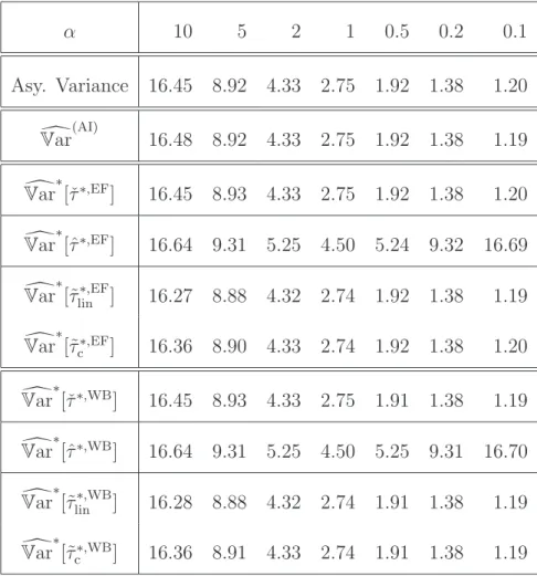
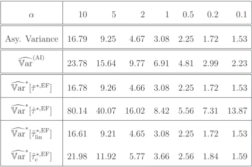
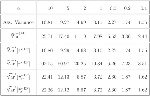
The validity of the weighted bootstrap is an asymptotic result. In particular, it hinges on the fact that asymptotically the actual bias is estimated consistently. The- oretically, this is achieved in Abadie and Imbens (2011) and Otsu and Rai (2017) by constructing a bias estimator based on flexible, nonparametric series regression estimators. In finite samples, one of course needs to choose the truncation param- eter in these series estimators, but, in practice, it is often advocated that using a linear regression with all the regressors or with their squares and crossproducts will be sufficient. These choices correspond to a series estimator using polynomial basis functions up to the first or second order only. In our simulations, we will demon- strate that such adhoc choices may lead to distorted inference results. We do so by varying the first two conditional moments in the distribution of the data. Using dif- ferent bias estimators, we are able to demonstrate the importance of doing accurate bias-correction for the weighted bootstrap to work properly. Finally, the simulations will also highlight the benefit of the properly performed weighted bootstrap vis-`a-vis the plug-in variance estimator proposed inAbadie and Imbens (2006).
The remainder of the paper is structured as follows. Section 2 provides the basic treatment effect setup along with the classical matching estimator and its bias- corrected version. The weighted bootstrap procedure of Otsu and Rai (2017) and some related resampling procedures are presented in Section 3. Some DGPs along with the corresponding distributional results of the nearest neighbor matching es- timator for the ATE are given in Section 4 allowing us to explicitly determine the asymptotic variance in our simulation study. Results pertaining to the behavior of
the weighted bootstrap are collected in Section5 including the main result showing that the key to validity is an appropriate bias-correction. The results of the simu- lation study to illustrate how the performance of the weighted bootstrap depends on the appropriateness of the estimated bias are given in Section6. Finally, Section 7 concludes. The detailed proofs are collected in the appendix at the end of the manuscript.
2 Setup
We consider the basic treatment effects setup. For each unit i = 1, . . . , N let Yi(0) and Yi(1) be the unobserved potential outcomes under control and after treat- ment, respectively. For each unit, we observe Zi = (Yi, Wi, Xi), where Wi is the treatment indicator (Wi = 1, if the unit is treated, and Wi = 0 otherwise), Yi = WiYi(1) + (1−Wi)Yi(0) is the observed outcome and Xi is a vector of (con- tinuously distributed) covariates. Let (Y(1), Y(0), W, X) be the population random variables. The observed data is drawn from (Y, W, X). Here, we are interested in estimating the the average treatment effect (ATE) given by
τ =E[Y(1)−Y(0)],
which is also the parameter of interest inOtsu and Rai(2017). LetZ:={(Yi, Wi, Xi)}Ni=1
be an i.i.d. random sample from the population (Y, W, X). The classical matching estimator for the ATE using M fixed matches with replacement is given by
ˆ τ = 1
N XN
i=1
{Yˆi(1)−Yˆi(0)}, (2.1) where
Yˆi(1) =WiYi+ (1−Wi) X
j∈JM(i)
Yj
M
and
Yˆi(0) =Wi
X
j∈JM(i)
Yj
M + (1−Wi)Yi
are imputation based estimates of the potential outcomes with JM(i) the index set of the first M matches for uniti
JM(i) =
j ∈ {1, . . . , N}:Wj = 1−Wi, X
l:Wl=Wj
1{||Xl−Xi|| ≤ ||Xj−Xi||} ≤M . Finally, with KM(i) =PN
l=11(j ∈ JM(l)) denoting the number of times unit i was a match, the classical matching estimator can be written as
ˆ τ = 1
N XN
i=1
(2Wi−1)
1 + KM(i) M
Yi. (2.2)
In order to derive the asymptotic properties of the matching estimator ˆτ, it is typ- ically assumed that one has an i.i.d. sample. In addition, one typically assumes that the regressors are continuously distributed, that the so-called common support condition and certain moment conditions hold. Denote the first two conditional moments of the outcome given the treatment status and the covariate value by µ(w, x) = E[Y | W = w, X = x] and σ2(w, x) = Var[Y | W = w, X = x], then a typical set of conditions is given in Assumption 1.
Assumption 1. The data Z = {(Yi, Wi, X)}Ni=1consists of N i.i.d. draws from the distribution of (Y, W, X), where Y =W Y(1) + (1−W)Y(0) with:
(i) X is continuously distributed on a compact and convex set X ⊂ Rk. The density of X is bounded and bounded away from zero on X.
(ii) W is independent of (Y(0), Y(1)) conditional on X = x for almost every x ∈ X. There exists η > 0 such that Pr(W = 1 | X = x) ∈ (η,1−η) for almost every x∈X.
(iii) For each w ∈ {0,1}, µ(w,·) and σ2(w,·) are Lipschitz continuous on X; σ2(w,·) is bounded away from zero on X and E[Y4|W = w, X = ·] is uni- formly bounded on X.
These conditions correspond to the set of assumptions given inAbadie and Imbens (2006, 2011) and Otsu and Rai (2017). Identification of the ATE is guaranteed by the common support condition in Assumption 1(ii). Asymptotically, one could
weaken Assumption1(i) and allow for discretely distributed covariates taking finitely many values with all the results being established for subsamples based on the val- ues of the discrete covariates. In finite samples, allowing for discrete covariates in such a fashion may lead to difficulties as the common support condition may fail in the sample. In this case one could treat the discrete covariates as if they were continuously distributed. The smoothness conditions in Assumption 1(iii) are used to establish the consistency and asymptotic normality of the matching estimators.
Under the conditions in Assumption 1, Abadie and Imbens (2006) derived consis- tency and asymptotic normality of the classical matching estimator ˆτ. In particular, they established that
√N(ˆτ−BN −τ) σN
−→ Nd (0,1), where
σ2N = 1 N
XN i=1
1 + KM(i) M
2
σ2(Wi, Xi) +Eh
µ(1, X)−µ(0, X)−τ2i and the bias term is given by
BN = 1 N
XN i=1
2Wi−1 M
X
j∈JM(i)
µ(Xi,1−Wi)−µ(Xj,1−Wi)
= 1 N
XN i=1
(2Wi−1) µ(Xi,1−Wi)− 1 M
X
j∈JM(i)
µ(Xj,1−Wi) .
Moreover, they showed that unless one uses a single regressor (k = 1), the bias term BN of the classical matching estimator ˆτ dominates the asymptotic distribution and the classical matching estimator will not be √
N-consistent. In particular, under Assumption1, their Theorem 1 holds, which states thatBN =Op(N−1/k). The bias term depends on the conditional means in both treatment arms. Thus, if we have estimators for these conditional means, denoted by ˆµ(x, w) for w∈ {0,1}, then we can estimate the bias by
BbN = 1 N
XN i=1
2Wi−1 M
X
j∈JM(i)
ˆ
µ(Xi,1−Wi)−µ(Xˆ j,1−Wi)
(2.3) and we can define the bias-corrected matching estimator by ˜τ := ˆτ − BbN. It is immediately clear that if the bias estimator can be shown to satisfy√
N( ˆBN−BN) =
oP(1), then it follows that
√N(˜τ −τ) σN
−→ Nd (0,1).
Abadie and Imbens (2011) use a flexible, nonparametric series regression estima- tor to estimate the conditional means and provide sufficient conditions to ensure
√N( ˆBN −BN) = oP(1). Plugging-in (2.2) and (2.3) and re-arranging, the bias- corrected matching estimator can be written as
˜ τ = 1
N XN
i=1
(2Wi−1)
1 + KM(i) M
Yi−µ(Xˆ i, Wi) + (2Wi−1) ˆµ(Xi, Wi)−µ(Xˆ i,1−Wi)
=: 1 N
XN i=1
˜
τi, (2.4)
where we will call
˜
τi = (2Wi−1)
1 + KM(i) M
Yi−µ(Xˆ i, Wi)
+ (2Wi−1) ˆµ(Xi, Wi)−µ(Xˆ i,1−Wi) (2.5) the individual contribution to the bias-corrected matching estimator. Similarly, we can write
ˆ τ = 1
N XN
i=1
(2Wi−1)
1 + KM(i) M
Yi =: 1 N
XN i=1
ˆ
τi, (2.6)
and will call
ˆ
τi = (2Wi−1)
1 + KM(i) M
Yi (2.7)
the individual contribution to the classical matching estimator.
3 The weighted bootstrap estimator
The weighted bootstrap estimator proposed byOtsu and Rai (2017) is defined as a randomly weighted average of the difference between the individual contributions of the bias-corrected matching estimator and the bias-corrected estimator. Recalling the decomposition of the bias-corrected matching estimator in (2.4) in terms of the
individual contributions given in (2.5) the weighted bootstrap estimator is defined as
√NT˜∗ = XN
i=1
ηi∗(˜τi−τ˜), (3.1) for a given choice of randomly drawn resampling weights η∗i, i= 1, . . . , N.
In order to derive the validity of the weighted bootstrap,Otsu and Rai (2017) con- sider the setting of Abadie and Imbens (2011). In particular, the conditions in Assumption1are assumed to hold, the bias is estimated using nonparametric series estimators ˆµ(x, w), forw∈ {0,1}and the conditions ensuring that√
N( ˆBN−BN) = op(1) are satisfied. In this setup, Otsu and Rai (2017) showed that, whenever the resampling weights satisfy the conditions given in Assumption2, the weighted boot- strap is valid in the sense that d(√
NT˜∗,√
N(˜τ−τ))−→P 0 withd the Kolmogorov distance.
Assumption 2. The resampling weights η∗i, i= 1, . . . , N satisfy:
(i) (η1∗, . . . , η∗N)is exchangeable and independent of the dataZ={(Yi, Wi, Xi)}Ni=1. (ii) PN
i=1(ηi∗−η∗)2 −→P∗ 1, where η∗ = N1 PN i=1ηi
(iii) maxi=1,...,N|ηi∗−η∗|−→P∗ 0.
(iv) E∗ (ηi∗)2
=O(N−1) for all i= 1, . . . , N. Choosing wild bootstrap-type weights ηi∗ =ǫ∗i/√
N, where {ǫ∗i}Ni=1 are i.i.d. random variables with a zero mean and unit variance is admissible in Assumption 2. By calling the resulting procedure based on this choice of weights the wild bootstrap, allows Otsu and Rai (2017) to conclude that the conjecture of Abadie and Imbens (2008) has been formally confirmed.
However, the conditions in Assumption 2 also allow for the choice of ηi∗ =Mi∗/√ N with (M1∗, . . . , MN∗) a multinomially distributed random vector based on N trials and N equally likely cells. This choice of resampling weights is nothing else but a rescaling of a simple Efron bootstrap applied to (˜τi,c, i = 1, . . . , N), where ˜τi,c :=
˜
τi−τ˜ as
XN i=1
Mi∗
√N(˜τi−τ˜) = 1
√N XN
i=1
Mi∗τ˜i,c = 1
√N XN
i=1
˜ τi,c∗
where (˜τi,c∗ , i = 1, . . . , N) denotes an Efron bootstrap sample obtained by indepen- dently drawing with replacement from (˜τi,c, i = 1, . . . , N). In fact, it can even be written in terms of a simple Efron bootstrap of the individual contributions of the bias-corrected matching estimator asPN
i=1Mi∗ =N implies that
√1 N
XN i=1
Mi∗(˜τi−τ˜) = 1
√N XN
i=1
Mi∗τ˜i−√
Nτ˜= 1
√N XN
i=1
˜ τi∗−√
Nτ˜
where (˜τi∗, i = 1, . . . , N) is an Efron bootstrap sample obtained by independently drawing with replacement from the (uncentered) individual contributions (˜τi, i = 1, . . . , N).
As the choice of the weights is not restricted to the wild bootstrap-type weights and an Efron bootstrap of the (˜τi,c, i= 1, . . . , N) is also valid, this already indicates that it is not the “wildness” that makes the weighted bootstrap procedure work. In fact, as we will see Section 5the key for the validity is that the bias-corrected individual contributions are resampled as opposed to resampling the individual contributions of the classical matching estimator or to resampling the original data.
In the last part of this section we will show in what way the valid bootstrap estimator using Efron-type weights can be interpreted as an Efron bootstrap based on an
“augmented” data set. The naive Efron-type bootstrap of the data{(Yi, Wi, Xi)}Ni=1
considered in Abadie and Imbens (2008) fails because the bootstrap counterpart of KM(i) fails to correctly reproduce the matching distribution KM(i). As a possible solution, it may be conceivable to use an Efron bootstrap that treates the matches KM(i) as a characteristic of the original data. However, if one uses an Efron-type bootstrap on the “augmented” data {(Yi, Wi, Xi, KM(i))}Ni=1 and then plugs in the bootstrap variables into the formula of the classical matching estimator, we get exactly the same as using an Efron bootstrap on the individual contributions of the classical matching estimator
√NTˆ∗ = XN
i=1
Mi∗
√N(ˆτi−τˆ) = 1
√N XN
i=1
ˆ
τi,c∗ = 1
√N XN
i=1
ˆ τi∗−√
Nτ ,ˆ (3.2) where (ˆτi,c∗ = ˆτ∗−τ , iˆ = 1, . . . , N) with (ˆτi∗, i= 1, . . . , N) the Efron bootstrap sample of the individual contributions of the classical matching estimator. Thus, when the weighted bootstrap on the individual contributions of the classical matching
estimator is invalid, it is also invalid to use an Efron on the “augmented” data {(Yi, Wi, Xi, KM(i))}Ni=1 along with the formula for the classical matching estimator – even in settings when the classical matching estimator is unbiased in finite samples.
Finally, from
√NT˜∗ = XN
i=1
Mi∗
√N(˜τi−τ˜) = 1
√N XN
i=1
˜
τi,c∗ = 1
√N XN
i=1
˜ τi∗−√
Nτ .˜
we see that the valid weighted bootstrap with Efron-type weights can be interpreted as an Efron bootstrap on the “augmented” data {(Yi, Wi, Xi, KM(i))}Ni=1 that uses the formula of the bias-corrected estimator. Notice, that the bias-correction is not re-calculated in the bootstrap sample, so that this is another “characteristic” of the original data that is kept. Therefore, the weighted bootstrap with multinomially distributed weights, can be thought of as an Efron boostrap on the “augmented”
data {(Yi, Wi, Xi, KM(i),µ(Xˆ i, Wi),µ(Xˆ i,1−Wi)}Ni=1.
4 A simple DGP allowing for closed-form asymp- totic expressions for the ATE
In order to show that the bias-correction is necessary for the validity of the weighted bootstrap, we will follow in the vein of Abadie and Imbens (2008). In particular, we will consider a DGP for which the classical nearest neighbor matching estimator is unbiased even in finite samples and for which we can derive closed from expres- sions for (i) the limit variance of the nearest neighbor matching estimator and (ii) the limit of the expectation of the conditional variance of the weighted bootstrap when applied to the individual contributions of the classical matching estimator.
As these two expressions turn out to be different, this proves that a weighted boot- strap applied to the individual contributions of the classical matching estimator (without bias correction) is not valid, although the estimator is actually unbiased and, in particular, for the purpose of point estimation there is no bias to correct for. Note, that the simple expressions cannot be derived using the setup considered by Abadie and Imbens (2008), which was used to get corresponding results when estimating the ATET. We have to modify the DGP to allow for i.i.d. draws from
(Y, W, X). In particular, this entails that we will no longer have a fixed ratio of treated to control units in the sample, which in turn makes the derivation of the expressions substantially more difficult.
Assumption 3. Let Z = {(Yi, Wi, Xi)}Ni=1 =: (Y,W,X) be a sample of N inde- pendent draws from (Y, W, X), where:
(i) The regressor satisfies X ∼ U[0,1].
(ii) W ∼ Bern(p) with p=α/(1 +α) for some finite positive α.
(iii) Y =W Y(1) + (1−W)Y(0) with the potential outcomes satisfying:
(a) Y(1) is degenerate with Pr(Y(1) = c) = 1 for some fixed c.
(b) Y(0) |X =x∼ N(0,1) for all x∈[0,1].
As we are only considering one continuous covariate in Assumption3, we know that
√NBN =oP(1), so that it will not contribute to the asymptotic distribution of the classical matching estimator. In fact, as µ(x,0) = 0 and µ(x,1) = c for all x the bias of the classical matching estimator is exactly zero, because
BN = 1 N
XN i=1
(2Wi−1) 1 M
X
j∈J(i)
µ(Xi,1−Wi)−µ(Xj,1−Wi)
= 0.
Assumption 3(iii) implies that the ATE τ equals c. It thus follows that
√N(ˆτ −τ) σN
−→ Nd (0,1),
where, becauseµ(x,1)−µ(x,0)−τ = 0, σ2(x,1) = 0 and σ2(x,0) = 1 for all x, we have
σN2 = 1 N
XN i=1
1 + KM(i) M
2
σ2(Xi, Wi) +Eh
µ(X,1)−µ(X,0)−τ2i
= 1 N
XN i=1
(1−Wi)
1 + KM(i) M
2
.
In the following, we will consider the nearest neighbor matching estimator based on a single match, that is withM = 1. To lighten notation, we will writeKi :=K1(i).
In this case, it is possible to establish the distributional results for the matching estimator of the ATE under Assumption 3.
Proposition 1 (Distributional results for nearest neighbor matching estimator ˆτ).
Given Assumption 3 the nearest neighbor matching estimator for the ATE, ˆ
τ = 1 N
XN i=1
(2Wi −1) (1 +Ki)Yi
satisfies
√N(ˆτ−τ)−→ Nd
0,1 + α 1 +α
2 + 3
2α
.
The proposition can be seen as a companion result to the simple expressions derived by Abadie and Imbens (2008) in the ATET case. In order to derive the results in the ATE case given in Proposition 1, we have to modify their proposed DGP, which then requires the use of substantially more complicated arguments based on some non-trivial results on asymptotic approximations for reciprocal moments of binomial random variables. From the proposition we can see that the classical nearest neighbor matching estimator is asymptotically normal with a limit variance that depends solely on the parameterα, which governs the expected ratio of treated to control units in the sample. Under the additional assumption that the bias estimatorBbN satisfies√
N(BbN−BN) =√
NBbN =oP(1), the bias-corrected nearest neighbor matching estimator with (M = 1) will have the same asymptotic limit, that is
√N(˜τ−τ)−→ Nd
0,1 + α 1 +α
2 + 3
2α
.
Proof of Proposition 1. Given the DGP in Assumption3, we have already seen that the ATEτ is given byc. Some simple calculations show that for the classical nearest neighbor matching estimator under the DGP of Assumption 3one gets
ˆ τ = 1
N XN
i=1
Wi(1 +Ki)τ −(1−Wi) (1 +Ki)Yi(0)
=τ −(1−Wi) (1 +Ki)Yi(0), where the last line follows from PN
i=1Wi +PN
i=1KiWi = N1 +N0 = N. Thus ˆ
τ−τ =−N1 PN
i=1(1−Wi) (1 +Ki)Yi(0) and and it follows that
√N(ˆτ−τ)|W,X∼ N 0, 1 N
XN i=1
(1−Wi) (1 +Ki)2
! .
The total law of variance leaves us with Var[√
N(ˆτ−τ)] =Eh Var[√
N(ˆτ−τ)|X,W]i
+Varh E[√
N(ˆτ−τ)|X,W]i
=E
"
1 N
XN i=1
(1−Wi) (1 +Ki)2
# .
Thus, we are left to show that the last expression converges to the limit variance given in the proposition. As {Wi}Ni=1 are i.i.d. and the {Ki}Ni=1 are exchangeable, we get
Var[√
N(ˆτ−τ)] =E[1−Wi] + 2E[(1−Wi)Ki] +E[(1−Wi)Ki2]
= 1
1 +α 1 + 2E[Ki |Wi = 0] +E[Ki2 |Wi = 0]
.
When deriving the limit expressions of the termsE[Ki |Wi = 0] andE[Ki2 |Wi = 0]
we cannot directly appeal to the results in Abadie and Imbens (2008) as there, N0
andN1, the number of control units and treated units are assumed to be fixed frac- tions of the sample size. Instead, we have to use a conditioning argument and results on asymptotic expansions of reciprocal moments of binomial random variables to get
E[Ki |Wi = 0] →α and E[Ki2 |Wi = 0]→α+ 3
2α2 (4.1)
asN → ∞from which the proposition follows. The details of the lengthy technical arguments leading to (4.1) are given in Appendix A.
The setting in Assumption3will serve to show that the weighted bootstrap applied to the individual contributions of the classical matching estimator (without bias correction) is not valid even if the classical matching estimator is unbiased in finite samples.
In Section6, we will use simulations to investigate the performance of the weighted bootstrap estimator when the bias is poorly estimated. In order to do so, we will consider DGPs that satisy Assumption 4, where (iii)(b) in Assumption 3 has been replaced by Y(0)|X = x ∼ N(µ(x,0), σ2(x,0)) for specific choices of µ(x,0) and σ(x,0). Note, that if µ(x,0) = 0 andσ2(x,0) = 1, then the conditions are the same as those in Assumption 3.
Assumption 4. Let Z = {(Yi, Wi, Xi)}Ni=1 =: (Y,W,X) be a sample of N inde- pendent draws from (Y, W, X), where:
(i) The regressor satisfies X ∼ U[0,1].
(ii) W ∼ Bern(p) with p=α/(1 +α) for some finite positive α.
(iii) Y =W Y(1) + (1−W)Y(0) with the potential outcomes satisfying:
(a) Y(1) is degenerate with Pr(Y(1) = c) = 1 for some fixed c.
(b) Y(0)|X = x ∼ N(µ(x,0), σ2(x,0)) for specific choices of µ(x,0) and σ(x,0).
Given any DGP satisfying Assumption4, we now get τ =c−E[µ(X,0)]. As we are still only considering one regressor, i.e.BN =Op(N−1), so that the bias will still not contribute to the asymptotic distribution of the classical nearest neighbor matching estimator. Moreover, we get
√N(ˆτ−τ) σN
−→ Nd (0,1) where (using σ2(x,1) = 0 and µ(x,1) =c), we have
σ2N = 1 N
XN i=1
(1 +Ki)2σ2(Xi, Wi) +Eh
µ(X,1)−µ(X,0)−τ2i
= 1 N
XN i=1
(1−Wi) (1 +Ki)2σ2(Xi,0) +Eh
µ(X,0)−E[µ(X,0)]2i .
Although the expression forσ2N is more complicated than under the more restrictive Assumption 3, it is still possible to calculate the limit of its expectation as in the proof of Proposition1provided µ(x,0) and σ2(x,0) are polynomials in x. In partic- ular, as the Ki depend on the regressors in the treated group and these are drawn independently of the control observations, we haveE[(1−Wi)(1 +Ki)2σ2(0, Xi)] = E[(1−Wi)(1+Ki)2]E[σ2(0, Xi)]. Thus, in addition to the steps of the proof of Propo- sition 1, one has to calculate certain moments of a uniformly distributed random variable.
5 Bias-correction affects bootstrap validity
In this section we prove that the weighted bootstrap without bias-correction is in general invalid. We will do so by considering the setting of Assumption 3, where the classical matching estimator is already unbiased even in finite samples. In this setting we will derive the limit of the expectation of the conditional variance of the weighted bootstrap based on resampling the individual contributions of the classical matching estimator (without bias correction) and see that it does not converge to the correct limit.
Denote byE∗[·] andVar∗[··] the expectation and the variance, respectively, over the resampling mechanism conditional on the orginal data. Now, suppose that the DGP is given as in Assumption 3 and that the bias estimator based on series estimators ˆ
µ(x, w) for w ∈ {0,1} satisfies √
N(BbN − BN) = √
NBbN = oP(1). From the validity of the weighted bootstrap in this setting, we know thatEh
Var∗h√
NT˜∗ii
→ 1 + 1+αα 2 + 32α
for any choice of resampling weights satisfying Assumption 2.
Next, we will see that although the classical matching estimator is unbiased in the setting of Assumption 3, a weighted bootstrap procedure based on resampling the individual contributions of the classical nearest neighbor matching estimator will not be valid. Specifically, given the decomposition of the classical nearest neighbor matching estimator for the ATE in (2.6) in terms of the individual contributions, we will show that the conditional variance of the weighted bootstrap estimator based on resampling the corresponding contributions given in (2.7) will not converge to the correct limit. In particular, we will consider the weighted bootstrap procedure
√NTˆ∗ := 1
√N XN
i=1
ǫ∗i(ˆτi−τ)ˆ (5.1) with {ǫ∗i}Ni=1 a sequence of i.i.d. random variables that are independent of the data with E∗[ǫ∗i] = 0 and Var∗[ǫ∗i] = 1. Hence, this weighted bootstrap corresponds to a weighted bootstrap using wild bootstrap weights applied to the individual contributions of the classical matching estimator.
Theorem 1(Inconsistency of√
NTˆ∗). Under the DGP of Assumption3, the weighted bootstrap on the individual contributions of the classical nearest neighbor matching