A General Regression Procedure for Method Transformation. Application of Linear Regression Procedures for Method Comparison Studies in Clinical Chemistry, Part III

J. Clin. Chem. Clin. Biochem.

Vol. 26, 1988, pp. 783-790

© 1988 Walter de Gruyter & Co.

Berlin · New York

A General Regression Procedure for Method Transformation

Application of Linear Regression Procedures for Method Comparison Studies in Clinical Chemistry, Part III

By W. Bablok

Biometrie Diagnostica, Boehringer Mannheim GmbH, Mannheim H. Passing

Abt. Informatik und Kommunikation I Software, Hoechst AG, Frankfurt I Main 80 R. Bender

Techn. Wiss. Informationsverarbeitung, E. Merck, Darmstadt and B. Schneider

Abteilung Biometrie, Medizinische Hochschule Hannover

(Received March 16, 1987/May 17/August 22, 1988)

Summary: The bioinetrical treatment of laboratory data may require the estimation of a regression line for the transformation of one set of measurements to another. The regression procedure introduced in part I (1) of our work does not always yield unbiased results in such situations, since its estimators are not scale invariant. In part III we present the parameter estimation of a general regression equation which is scale invariant and retains all properties of the method comparison procedure, in particular its robustness. Its application is demonstrated by several examples, and the results are compared with other robust biometrical procedures. The mathematical aspects are explained in the appendix.

Introduction .. . . .corresponding to a positive value of Kendaffs τ (3), ^r „ , .„ ^/ON In the first part (1) of this series of papers we intro- it produces estimates which are not influenced by the duced a new biometrical regression procedure for the distribution of the data or the presence of biased or evaluation of method comparisons. It is used to de- extreme data points. In addition, parameter estima- termine whether measurements by two methods give tion and the statistical test results are independent of the same results apart from random errors, or show the assignment of the methods to the variables.

a systematic difference. In part II (2) we discussed its

properties and compared them with those of other There are situations in a clinical laboratory or in established regression procedures. Based on a linear research which require the transformation of one set structural relationship model, the procedure presented of measurements to another. This is the case when there can be used to test the hypotheses H0: β = 1 one wants to transfer the data from one system or and α == 0. Given a significant positive correlation reaction principle to another (e. g. different reaction

J. Clin. Chem. Clin. Biochem. / Vol. 26,1988 / No. 11

conditions, reagents or units, different activities or mass concentrations, etc). As we pointed out previ- ously (2), our regression procedure for method com- parison should not be used for this task. The esti- mators are biased since they are not scale invariant.

This is caused by the elimination of slopes with a value of - 1 and shifting the median by the number of slopes with a value smaller than -1. In part III we present two versions of a general regression pro- cedure which is scale invariant and possesses all the properties of the method comparison procedure. Ob- viously, it allows the estimation of a regression line with a negative slope. A detailed description is given in the next section; readers who do not wish to get involved in the mathematical aspects are recom- mended to proceed to section "Properties of the Regression Procedure".

Generalisation of the Estimation Procedure

For an experimental design as described in 1. c. (1, 2), we use the linear structural relationship model

y = α with χι = χ*

βχΓ

and = y* + (i = 1, ..., n).

χΓ and yi* are the expected values of the i-th sample of method 1 and method 2, respectively. They have an arbitrary but continuous distribution over all pos- sible samples, ξί and τ[^{ are the measurement errors of the i-th sample. For their variances the relationship

^ = ² (Eq.l)

is assumed. For the derivation of the regression pro- cedure we start with the assumption of a positive correlation, i. e. that KendalFs τ is significantly greater than zero.

Definition under the assumption of τ > 0 Firstly we deal with the estimation b of β. For 1 < i

< j < η we calculate all slopes Sy in the following way:

S« =

YJ - Yj

— co + oo - 0 + 0

if Yi Φ YJ and Xi Φ Xj if yi < ^ and Xi = Xj

if yi > yj and ^ = Xj (Eq. 2) if Yi = Yj and *i < Xj

if Yi = Yj and Xi > Xj

The Sy are sorted with the convention of — 0 < +0 leading to

S(3) < S(2) < ... < S(N)

where Ν denotes all possible slopes according to Eq. 2.

In analogy to part I (1) we define tor a suitable Κ if N odd

b(K): = (Eq.3)

ifNeven

It follows that b(K) is the median of the sequence

When Ν is even, the median is defined by the geo- metric mean, in order to guarantee an exact numerical independence of method assignment. Since slopes with values —0 and +0 and +00 and — oo are adjacent in this sequence, the choice of the index for any given data point (x^is yO has no influence on the result. As a consequence^ the definition (Eq. 2) of the Sy is meaningful.

We shall show in the appendix that the offset Κ has to meet a simple condition in order to make b(K) independent of the assignment of the methods to the variables. All the Κ meeting this condition define a family of regression procedures.

We distinguish between two alternative definitions of K. For the notation we use square brackets to denote with [a] the greatest integer smaller or equal to a non- negative real number a and the symbol # to describe the number of elements in a set.

Regression procedure 1

With neg : = # {Sy < - 0} we define

(Eq.4) and estimate b(K) by insertion of this Κ into Eq. 3.

Obviously, the indices are well defined. It is shown in the appendix that the computation can be simplified when τ > 0, provided there are no slopes with a value of 0 or oo.

With pos := #{S^y > 4- 0} b is estimated by S/pos + i\ if pos odd b =

/p

\

(Eq.5)

not defined if yj = yj and

/pos\ · S/pos \ if pos even provided that only the Sy > + 0 #re used.

Regression procedure 2 We define

K = #{S^(q) < - β} + [1/2 # {S«, = - β}]

(Eq.6) The indices are well defined as long as Kendalfs τ is significantly greater than zero (1). Since K in Eq. 6 depends on the unknown β, the slope b cannot be calculated from Eq. 3. Therefore we replace β in Eq. 6 by b and have

Κ = #{S(q) < - b} + [1/2 · #{S(q) = - b}].

(Eq.7) It follows that b and Κ are implicitly defined as solutions of the equations Eq. 3 and Eq. 7; they have only one solution as we shall show in the appendix.

To get to the solution we define an iterative process.

It starts with estimating b as in part I (1) and calcu- lates the sequence (Kr, br) from Eq. 7 and Eq. 3:

Ki = *{S^(q) < - 1}, b, = b(K,);

K^r = #{S^(q) < _ b^r_!} + [1/2 - *{S^(q) = - b^r_J], br = b(Kr); (Eq. 8) forr = 2, 3, ...

Since the set of slopes Sy is finite the sequence of the b^r must be periodic, that is, there must be an m > 1 and an r* > 1 with bm + r* == br*. If such an m and r* is found the iteration procedure stops and we get

b = ^

-I- m/2) if m even

V b/. m -1\ · b/. (*+-r) (

r + if m odd(Eq. 9) It is easy to show by mathematical induction that either m = 1 or m = 2 is true under the assumption of continuously distributed data. With b defined by Eq. 9, we calculate K according to Eq. 7.

Estimation of β with τ < 0

For a significant negative correlation we use the trans- formation

w,:= - γι, i = 1,2, ..., n.

Then the Xi and Wj have a positive correlation, and the estimator b^w can be calculated as in the previous section if we replace y» by — w».

The estimator b of the slope between the ^ and ys is defined by

b = - bw.

Estimation of the intercept α

(Eq. 10)

As in part I (1), we estimate the intercept in such a way that at least half of the points (xi9 yO are located above or on the regression line and at least half of the points below or on the regression line. Therefore the estimator of α is given by

a = med {y^ — b

Confidence interval for β and α

(Eq.ll)

Because of equation 3 we can construct a confidence interval for β by

S(M, + Κ) < β < S(M2 + K) (Eq. 12) where M! and M² are defined as in part I (1).

The confidence interval for α is given in the same way by

(Eq. 13) med{yi - S(M2 + K) · Xi} < α

< med{yi - S^ + κ> · x«}.

Properties of the Regression Procedure Scale invariance of b

b is called scale invariant if, after transforming the data of one method by a factor f, the estimator b is transformed by the same factor. Equation 4 and 6 show that the value of Κ does not change when either the Xj or y\ are transformed. Because of equation 3, b is transformed in accordance with Xj or y». This proves the scale invariance for the estimators of both pro- cedures.

Robustness of the estimators b and a

The definition of b and a as medians guarantees that there is no serious influence of extreme measurement points on the estimators. This property of the method comparison holds true for the regression procedures without restrictions.

Assignment of method 1 and 2 to variables X and Υ is interchangeable

In the appendix we show for both procedures that, after changing the assignment of the methods to X

J. Clin. Chem. Clin. Biochem. / Vol. 26,1988 / No. 11

and Y, b is transformed to 1/b and a to — a/b. This means that the estimated regression line can be solved for x, yielding parameters which equal those obtained for the estimators after interchanging the assignment of the methods.

Test for linearity

The assumption of a linear structural relationship can be tested after estimation of β and α by the cusum or run test. Details are given in 1. c. (1).

Discussion

In the previous section we described the properties of the two estimation procedures. For all data sets which we have processed so far with both procedures we found only negligible differences, if any, between the resulting estimates. In addition, we performed a sim- ulation study in analogy to that described in 1. c. (2) to compare the behaviour of both procedures when subjected to different data sets. There were only min- imal differences in the results. We recommend the use of procedure 1 to estimate the regression parameters, since it is easier to calculate than procedure 2.

The estimation of α and the test for linearity corre- sponds directly to what has been outlined in part I (1). A data set with a negative correlation is treated by transforming the yj and the resulting b according to section "Confidence interval for β and a". There- fore, the properties of the regression procedure as claimed in the introduction are proven. It should be noted that it does not make sense to compute a regression line for a structural relationship with a data set which is not significantly correlated. It is recommended to test the correlation before calculat- ing the regression line.

The regression procedure is not a special case of the method comparison procedure, even though it has been derived therefrom. Therefore the user needs a criterion for distinguishing between both: if a method comparison study has to be evaluated, then the pro- cedure described in part I should be used. It can be used to test the hypothesis that both methods are equal. To describe a general structural relationship between two methods (e. g. a method transformation), one of the procedures presented here should be ap- plied. We allow an input of negative data for both procedures, but for the method comparison one has to consider whether negative values are meaningful for the common measurement range of both methods.

When the parameters of a general regression line are estimated, testing the hypothesis β = 1 does not make

Input data

Test Kendall's ΤΦ 0 Calculate and sort slopes Sjj Method comparison

Set b = b, Calculate a Test linearity Calculate confidence intervals for a and β Test β = 1 and a= ο

Set K, = # {Sjj <-1>

Remove S\] = - 1

Determine bj = med ( S ^ K , ) )

Method · t transformation Include Sjj = - 1

t

Set K² = *{5^ΰ<-|>,} + ...

t

Until br = ^.τ (or br_2 ):

Set K^r = #{S^rj <-b^r_,}+...

Determine br = med (S(q + Kr) )

+

Set b = br or Ybr br_;

Calculate a Test linearity Calculate confidence intervals for a and β

Fig. 1. Flow chart

sense. Therefore it should be decided before the eval- uation which regression problem has to be handled.

The differences in the calculation of a regression line for the method comparison or for the general case are shown in figure 1.

Another regression procedure of the structural rela-.

tionship model is the standardized principal compo- nent analysis (4, 5) which also makes it possible to interchange the assignment of the methods to the variables. As long as its assumptions regarding the distribution of the data and the error terms are met, it will yield reliable results. Since the estimators are easily calculated its use can be recommended for many situations. However as discussed in part II (2), ex- treme data points and skew distributions have a rather strong influence on the results. The orthogonal regres- sion which is recommended in the standardization of coagulation reagents (6) has the same drawbacks. It is the advantage of our procedure that it produces robust estimates, especially in situations described above.

Other approaches for robust regression procedures are known in the literature. Of interest here is the concept of Johnstone & Velleman (7) whose resistant line estimator for the slope b is easier to compute than the estimator presented in this paper. However, the independence of the assignment of the methods to the variables is not guaranteed. This is also the case for another robust regression procedure: Siegers repeated median estimator (8) is based on a vector of

slopes Sjj similar to that in our procedure, but it also depends on the assignment of the methods. Both of the above procedures have properties which may be useful in other applications. We consider the inter- change of the methods to the variables an essential demand for a suitable regression procedure in method conversion.

The properties of the procedures discussed here be- come evident for a data sample which has been ob- tained by measuring a substance with two different chemical reaction principles. It demonstrates how the estimates are effected by the distribution and variation of the data as well as by the assignment of the methods to the variables:

Tab. 1. Estimates of b and a from the regression procedures.

Regression procedure Assignment n = 41 40 39

Standardized principal component

Passing &. Bablok Johnstone & Velleman Siegel

y

=

f(x)

χ =

f(y)

y =

f(x)

χ =

f(y)

y =

f(x)

χ =

f(y)

y =

f(x)

χ =

f(y)

0.841.19 2.140.47 0.431.96 2.080.44

-1.611.91 -2.03

0.95 -1.65

1.26 -1.93

1.14

2.410.42 2.210.45 2.070.36 2.160.37

-2.83 1.17 -2.20

1.00 -1.79 1.30 -2.07

1.22

2.060.49 2.140.47 0.421.94 2.080.44

-1.83 0.89 -2.03

0.95 -1.53

1.29 -1.93 1.14

120

ι—ιin Ε 90

JQ

ΌΟ

60

30

r-,30in

ΌΟ

10

30 60 90

Method 1 Carb. units! 120 10 20 30

Method 1 Carb. units]

60

τ: 45

30

TD Ο

15

+ -f

15 30 45

Method 1 Carb. units] 60

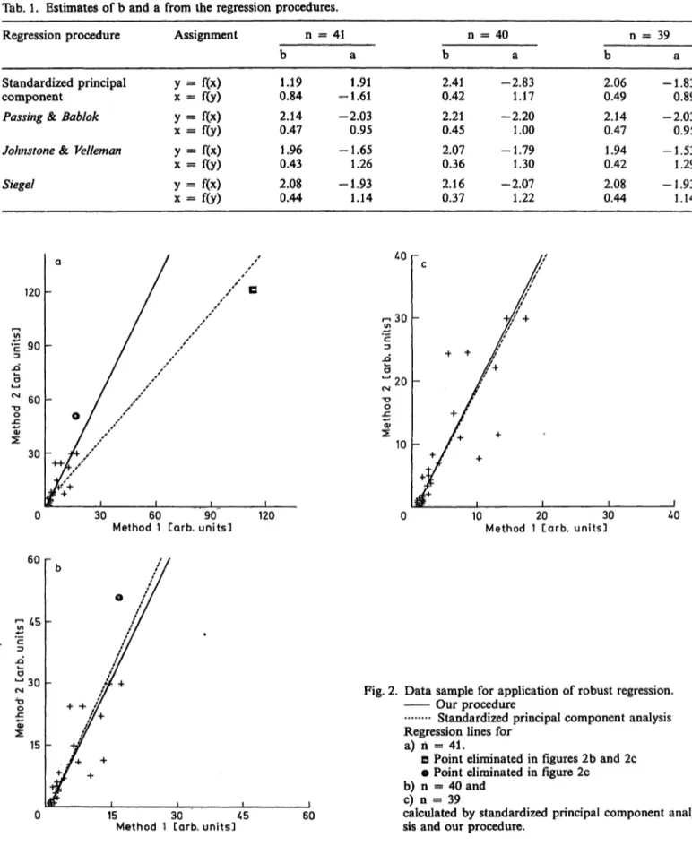
Fig. 2. Data sample for application of robust regression.

Our procedure

Standardized principal component analysis Regression lines for

a) ή = 41.

D Point eliminated in figures 2b and 2c e Point eliminated in figure 2c

b) n = 40 and c) n = 39

calculated by standardized principal component analy- sis and our procedure.

J. Clin. Chem. Clin. Biochem. / Vol. 26,1988 /No. 11

The increasing variation of the data in the upper concentration range produces an influence similar to that of extreme data points. If we eliminate the last and the last two data points we get three data sets with varying estimates for the Standardized Principal Component and robust estimates for the other pro- cedures. In contrast, if we change the assignment of the methods, the estimators of the procedures from Johnstone & Velleman and from Siegel differ from those obtained by solving the original equation for x.

The results are shown in table 1, the graphs of the data in figure 2.

The table shows that the other robust procedures estimate a value for b that cannot be transformed into its reciprocal. For example the Johnstone & Velle- man regression produces b = 1.96 and 1/b = 0.51 in contrast to B = 0.43 and 1/b = 2.33, with B as estimator for χ = f(y).

Application in Clinical Chemistry

There are many situations where a general regression procedure is needed in clinical chemistry for research and routine laboratory work. Frequently the linear regression is used without attention to the experimen- tal design and the resulting data from which the regression parameters are calculated. A discussion of the clinical and biochemical conditions, under which a linear tranformation based on a structural relation- ship model may be applied, goes beyond the limits of a statistical paper. However, it is intended to present

1600 -

^1200

-Ό_ο

JC

800

400

400 800 1200

Method 1 Carb. units] ¹⁶⁰⁰

some proposals elsewhere for further discussion (9).

To demonstrate the properties and the behaviour of our procedure we give a numerical example.

The regression procedure may be of use when two methods with different chemical reagent compositions are compared which measure the same analyte. It is possible to describe the results of one method with respect to the location of the other method, Another application could be in converting the results of an instrument with individual properties to a reference system with known properties. Clearly, any transfor- mation does only affect the location of the measure- ment points. The original degree of variation is not influenced by the calculation.

Mathematical Appendix

The independence of method assignment We derive a general condition for K which enables b(K) to be independent of the assignment. First of all we state the following definitions:

K(- oo) := # {S^(q) = - oo}, K(- 0) : = # {S(q) = - 0}and neg := # {S(q) < - 0}.

For a given K with K(- oo) < K < neg we define a partition of the set {S(q) < - 0} into four subsets:

• • • 5 S(K(-00))},

(- oo) + 1), ·-

{S(K +1), · - -, S(neg - K(- 0))}

{S(neg - K(- 0) + 1)» · - ·, S(neg)}.

After changing the assignment of the methods to X and Υ we get slopes

Xi — Xj

~

which are calculated analogously to Eq. 2. Sorting the TU we get

(2)

Defining

k(- oo) := {T^(q) = - 00} = K(- 0)

k(- 0) : = {T^(q) = - 0} = K(- oo) and

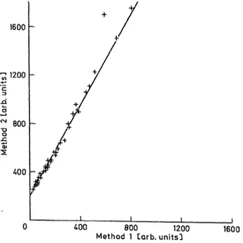
Fig. 3. Numerical example of method transformation. The line

represents y = 1.85 χ + 200. k(- oo) < k

we obtain for k with neg

a partition of the set {T(q) < - 0} in the same way as for the set {S(q) ^ — 0} and an estimation B(k) according to Eq. 3.

The assignment of the methods to X and Υ is arbi- trary, if and only if b = 1/B holds. For the proof we assume a positive correlation which can be obtained as outlined in section "Estimation of β with τ < 0"

in the case of τ < 0. For an odd Ν we find

Fr ¹ -)

(N + neg + l - iiyi - K)

l

and

It follows, that b = 1/B, if

k = neg - K. (Eq.13)

The same is true if N is even. Equation 13 defines a class of regression procedures. If K is computed as stated for regression procedure 1, then condition 13 is either exactly or approximately fulfilled. In the latter case, there is a gap of one place in the sorted sequence, this is without importance if n is not very small.

Computing K for regression procedure 2 we get from Eq.8

K + k = Φ {- oo < S(q) < - br} + # {- br <

S(q) < 0} + 2 · [1/2 - # {S(q) = -, br}]

= neg — ε with ε e {0, 1}.

It follows by mathematical induction that the assign- ment of the methods to X and Υ is also arbitrary for ε = 0. If ε = 1, then independence of assignment holds approximately for values of η that are not too small.

Simplified calculation of b in regression pro- cedure 1

Since b is estimated by the median of non-negative slopes, it has to be shown that the indices in Eq. 3 and Eq. 5 belong approximately to the same elements in the sorted sequence of the slopes.

For that we distinguish four cases dependent on an even or odd value of neg and pos as defined in section

"Definition under the assumption τ > 0":

Case 1: neg and pos are even, it follows for N/2 + K =

neg/2 + pos/2 + neg/2 = neg + pos/2 and N/2 + Κ + 1 =

neg/2 + pos/2 + neg/2 + 1 = neg + pos/2 + 1.

Case 2: neg is even and pos odd, it follows for (N + l)/2 + K =

neg/2 + (pos + l)/2 + neg/2 = neg + (pos +l)/2.

Case 3: neg is odd and pos even, it follows for (N + l)/2 + K =

(neg + l)/2 + pos/2 + (neg - l)/2 = neg + pos/2.

Case 4: neg and pos are odd, it follows for N/2 + Κ =

(neg + l)/2 + (pos - l)/2 + (neg - l)/2 = neg + (pos — l)/2 and

N/2 + 1 + Κ =

(neg + l)/2 + (pos + l)/2 + (neg - l)/2 = neg + (pos + l)/2.

In case 1 and 2 the indices in Eq. 3 and Eq. 5 refer to the same element, in case 3 and 4 there is a gap of about half a place in the sorted sequence of the slopes which has no real consequences on the result. How- ever, there is a problem, when Sy's are present with values ± oo or + 0, since the sign depends on the choice of indices for the data points.

Equations 3 and 7 have at most one solution Let us assume that there are two different solutions (K', b') and (K", b") of Eq. 3 and Eq. 7 with

K' = # {S^(q) < - b'} + [1/2 - Φ {S^(q) = - b'}], K" = * {S^(q) < - b"} + [1/2 - # {S^(q) = - b"}], and

b7 = b(K'), b" = b(K").

If b' = b" is true then K' = K" would follow from Eq. 14 in contradiction to our assumption. Now let b' < b", then from Eq. 14 we get K' > K" and be- cause of Eq. 3 the contradiction b' > b". The analo- gous contradiction follows from the assumption b' > b" which proves that there is at most one solu- tion.

J. Clin. Chem. Clin. Biochem. / Vol. 26,1988 / No. 11

Is there always an exact solution of equations 3 and 7?

If all 8ϋ > 0 then K = 0 and b(0) = med{Sij} satisfy the equations 3 and 7. One can construct examples for which a solution of equations 3 and 7 does not exist even though τ is significantly greater than zero.

For instance the following data set has this property:

{(0,6), (3,1), (5,6), (7,8), (8,15)}

To explain this peculiarity we have to consider that to every K an interval of b's satisfies equation 6, whereas equation 3 defines for every Κ exactly one b. If there is a K with a solution b for Eq. 3 in an interval according to Eq. 7, then the pair (K, b) is the

exact solution. f

An MS-DOS program version for the regression pro- cedures is available on request.

References

1. Passing, H. & Bablok, W. (1983) J. Clin. Chera. Clin.

Biochem. 2L 709-720.

2. Passing, H. & Bablok, W. (1984) J. Clin. Chem. Clin.

Biochem. 22,431-445.

3. Hollander, M. & Wolfe, D. A. (1973) Nonparametric Statis- tical Methods, J. Wiley & Sons, New York.

4. Feldmann, U., Schneider, B., Klinkers, H. & Haeckel, R.

(1981) J. Clin. Chem. Clin. Biochem. 19, 121-137.

5. Averdunk, R. &' Borner, K. (1970) Z. Klin. Chem. Klin.

Biochem. 8, 263-268.

6. Loeliger, Ε. Α., van den Besselaar, T., Hermans, J. & van der Velde, E. A. (1984), BCR information No. 147, 148 and 149, Commission of the European Communities, Brussels.

7. Johnstone, I. M. & Velleman, P. F. (1985) J. Am. Statist.

Association 80, 1041 — 1054.

8. Siegel, A. F., (1982) Biometrika 69, 242^244.

9. Eisenwiener, H.-G., Bablok, W, Bender R., Passing, H., Sowodniok, B., Spaethe, R. & V lkert, E. (in preparation) Die Umrechnung von Methoden und Verfahren.

W. Bablok

c/o Boehringer Mannheim GmbH Sandhofer Stra e 116

D-6800 Mannheim 31