Summary of Linear Regression
1 Simple linear Regression
a Themodelof simple linear regression reads
Yi=α+βxi+Ei .
xi are fixed numbers, Ei are random, called “random deviations” or “random errors”.
(Usual) assumptions are
Ei∼ N h0, σ2i, Ei, Ek independent
The parameters of the model are the coefficients α, β and the standard deviation σ of the random error.
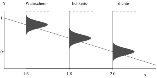
Figur 1.a shows the model. It is useful to imagine simulated datasets.
1.6 1.8 2.0
0 1
x
Y Wahrschein- lichkeits- dichte
Figure 1.a: Display of the probability model Yi = 4−2xi+Ei for 3 observations Y1, Y2 and Y3 corresponding to the x values x1= 1.6, x2 = 1.8 and x3 = 2
b Estimation of the coefficientsfollows the principle ofLeast Squares, which is derived from the principle of Maximum Likelihood under the assumption of a normal distribution of the errors. It yields
βb= Pn
i=1(Yi−Y)(xi−x) Pn
i=1(xi−x)2 , αb=Y −β x .b Estimates are normally distributed,
βb∼ N hβ, σ2/SSQ(X)i, αb∼ ND
α, σ2
1
n+x2/SSQ(X)E , SSQ(X) = Xn
i=1(xi−x)2 .
Thus, they are unbiased. Given that the model is correct, their variances are the smallest possible (among all unbiased estimators).
4 Statistik fr Chemie-Ing., Regression c The deviations of the observed Yi from thefitted values ybi=α+b βxb i are calledresiduals
Ri =Yi−byi and are “estimators” of the random errors Ei. They lead to an estimate of the standard deviation σ of the error,
b
σ2= 1 n−2
Xn i=1
Ri2.
d Testof the null hypothesis β =β0: The test statistic T = βb−β0
se(β) , se(β)= q
b
σ2/SSQ(X)
has a t distribution with n−2 degrees of freedom.
This leads to the confidence interval
βb±qt0.975n−2 se(β), se(β)=σ/b q
SSQ(X). Program output: see multiple regression.
e The “confidence band” for the value of the regression function connects the end points of the confidence intervals for EhY|xi=α+βx.
A prediction interval shall include a (yet unknown) value Y0 of the response variable for a given x0 – with a given “statistical certainty” (usually 95%). Connecting the end points for all possible x0 produces the “prediction band”.
2 Multiple linear Regression
a Themodel is
Yi = β0+β1x(1)i +β2x(2)i +...+βmx(m)i +Ei
Ei ∼ N h0, σ2i, Ei, Ek independent. Inmatrix notation:
Y = fXβe+E , E∼ Nnh0, σ2Ii. b Estimation is again based on Least Squares,
βb= (fXTfX)−1fXTY . From the distribution of the estimated coefficients,
βbj ∼ N
βj, σ2
(fXTXf)−1
jj
t-tests and confidence intervals for individual coefficients are derived.
The standard deviation σ is estimated by b
σ2 =Xn i=1R2i.
(n−p).
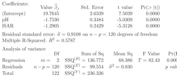
c Tabelle 2.c shows anoutput, annotated with the mathematical symbols.
The multiple correlation R is the correlation between the fitted values byi and the observed values Yi. Its square measures the portion of the variance of the Yis that is
“explained by the regression”,
R2 = 1−SSQ(E)/SSQ(Y) and is therefore called coefficient of determination.
Coefficients:
Value βbj Std. Error t value Pr(>|t|)
(Intercept) 19.7645 2.6339 7.5039 0.0000
pH -1.7530 0.3484 -5.0309 0.0000
lSAR -1.2905 0.2429 -5.3128 0.0000
Residual standard error: σb= 0.9108 onn−p= 120 degrees of freedom Multiple R-Squared: R2 = 0.5787
Analysis of variance
Df Sum of Sq Mean Sq F Value Pr(F)
Regression m= 2 SSQ(R) = 136.772 68.386 T = 82.43 0.0000 Residuals n−p= 120 SSQ(E) = 99.554 σb2 = 0.830 p value
Total 122 SSQ(Y) = 236.326
Table 2.c: Output for a regression example, annotated with mathematical symbols d Multiplicity of applications. The model of multiple linear regression model is suitable
for describing many different situations:
• Transformations of the X- (and Y-) variables may turn originally non-linear relations into linear ones.
• A comparison of two groups is obtained by using a binaryX variable. Several groups need a “block of dummy variables” to be introduced into the multiple regression model. Thus, nominal (or categorical) explanatory variablescan be used in the model and combined with continuous variables.
• The idea of different linear relations of Y with some Xs in different groups of data can be encluded into a single model. More generally, interactions between explanatory variables can be incorporated by suitable terms in the model.
• polynomial regressionis a special case of multiple linear (!) regression.
e The F test for comparison of models allows for testing whether several coefficients are zero. This is needed for testing whether a categorical variable has an influence on the response.
6 Statistik fr Chemie-Ing., Regression
3 Residual analysis
a The assumptions about the errors of the regression model can be split into (a) their expected values are EhEii= 0 (or: the regression function is correct), (b) they all have the same scatter, varhEii=σ2,
(c) they are normally distributed.
(d) they are independent of each other.
These assumptions should be checked for
• deriving a better model based on deviations from it,
• justifying tests and confidence intervals.
Deviations are detected by inspecting graphical displays. Tests for assumptions play a less important role.
b The following displays are useful:
(a) Non-linearities: Scatterplot of (unstandardized) residuals against fitted values (Tukey-Anscombe plot) and against the (original)explanatory variables.
Interactions: Pseudo-threedimensional diagram of the (unstandardized) residuals against pairs of explanatory variables.
(b) Equal scatter: Scatterplot of (standardized) absolute residuals against fitted values (Tukey-Anscombe plot) and against (original) explanatory variables. (Usu- ally no special displays are given, but scatter is examined in the plots for (a).) (c) Normal distribution: Q-Q-plot(or histogram) of (standardized) residuals.
(d) Independence: (unstandardized) residuals against time or location.
(*) Influential observationsfor the fit: Scatterplot of (standardized) residuals against leverage.
Influential observations for individual coefficients: added-variable plot.
(*) Collinearities: Scatterplot matrix of explanatory variables and numerical output (of R2j or VIFj or “tolerance”).
c Remedies:
• Transformation (monotone non-linear) of the response: if the distribution of the residuals is skewed, for non-linearities (if suitable), unequal variances.
• Transformation(non-linear) of explanatory variables: when seeing non-linearities, high leverages (can come from skewed distribution of explanatory variables) and in- teractions (may disappear when variables are transformed).
• Additional terms: to model non-linearities and interactions.
• Linear transformations of several explanatory variables: to avoid collinearities.
• Weighted regression: if variances are unequal.
• Checking the correctness of observations: for all outliers in any display.
• Rejection of outliers: if robust methods are not available (see below).
More advanced methods:
• Generalized Least Squares: to account for correlated random errors.
• Non-linear regression: if non-linearities are observed and transformations of variables do not help or contradict a physically justified model.
• Robust regression: should always be used, suitable in the presence of outliers and/or long-tailed distributions.
Note that correlations among errors lead to wrong test results and confidence intervals which are most often too short.
d Fitting a regression model without examining the residuals is a risky exercise!
L Literature
a Short introduction into regression:
• The following (recommendable) general introductions into statistics contain a chap- ter on linear regression: Devore (2004), Rice (2007)
b Books on Regression:
• Recommended: Ryan (1997).
• Weisberg (2005) emphasizes the exploratory search for a suitable model and can be recommended as an introduction into practice of regression analysis with a lot of examples.
• Draper and Smith (1998): A classic that pays suitable attention to checking assump- tions.
• Sen and Srivastava (1990) and Hocking (1996): Discuss the mathematical theory, but also include practical aspect. Recommended for reader with interest in the mathematical basis of the methods.
c Spezial Hints
• Wetherill (1986) treats some spezial problems of multiple linear regression more extensively, includingcollinearity.
• Cook and Weisberg (1999) show how to develop a model (including non-linear ones) using graphical displays. It introduces a special software package (R-code) which goes along with the book.
• Harrell (2002) discusses exploratory model development in full breadth as promised by the title “Regression Modeling Strategies”.
• Fox (2002) introduced model development based on the software R.
• Exploratory data analysis was popularized by the book of Mosteller and Tukey (1977), which contains many clever ideas.
• Robust regression was first made available for practice in Rousseeuw and Leroy (1987). A more concise and deep treatment is contained in Maronna, Martin and Yohai (2006), which treats robust statistics in its whole breadth.