Local Correlation Methods for the Calculation of
Molecular Magnetic Properties
Dissertation
zur Erlangung des Doktorgrades der Naturwissenschaften (Dr. rer. nat.) der Fakultät
- Chemie und Pharmazie - der Universität Regensburg
vorgelegt von
Stefan Loibl
aus Niederwinkling im Jahr 2014
Tag des Kolloquiums: 09.05.2014
Diese Arbeit wurde angeleitet von: Prof. Dr. Martin Schütz Prüfungsausschuss
Vorsitzender: Prof. Dr. Manfred Scheer
Erstgutachter: Prof. Dr. Martin Schütz
Zweitgutachter: Prof. Dr. Alexander Auer
Drittprüfer: Prof. Dr. Bernhard Dick
Kapitel 3
Stefan Loibl and Martin Schütz
“NMR shielding tensors for density fitted local second-order
Møller-Plesset perturbation theory using gauge including atomic orbitals”
The Journal of Chemical Physics 137, 084107 (2012), doi: 10.1063/1.4744102
Kapitel 4 und 5
Stefan Loibl and Martin Schütz
“Magnetizability and rotational gtensors for density fitted local second-order Møller-Plesset perturbation theory using gauge-including
atomic orbitals”
The Journal of Chemical Physics 141, 024108 (2014), doi: 10.1063/1.4884959
An dieser Stelle möchte ich mich bei allen bedanken, die zum Entstehen dieser Arbeit beigetragen haben:
Prof. Dr. Martin Schütz für die Möglichkeit, dieses interessante und an- spruchsvolle Thema zu bearbeiten, und seine stete Förderung meiner wis- senschaftlichen Arbeit,
Prof. Dr. Alexander Auerfür seine Bereitschaft die Rolle des Zweitgutachters zu übernehmen,
Dr. Denis Usvyat für seine stete Hilfsbereitschaft, wissenschaftliche Prob- leme und Unklarheiten zu diskutieren,
Klaus Ziereis für seine prompte und unkomplizierte Hilfe in technischen Dingen,
Katrin LedermüllerundGero Wälzfür viele angenehme Stunden im gemein- samen Büro und in der Freizeit,
meinen KollegenThomas Merz,Oliver Masur,Matthias Hinreiner,David David undMartin Christlmaiersowie ehemalsDr. Marco Lorenzfür viele nette und anregende Gespräche.
Ganz besonders bedanken möchte ich mich bei meinen Eltern Mariaund Karl, die mir mein Studium und die anschließende Promotion ermöglicht haben und bei meiner FrauElisabethfür Ihre stets liebevolle Unterstützung und Motivation.
vii
Publications
S. Loibland M. Schütz
“Magnetizability and rotational g tensors for density fitted local second- order Møller-Plesset perturbation theory using gauge-including atomic orbitals”
The Journal of Chemical Physics,141, 024108 (2014), doi: 10.1063/1.4884959 S. Loibland M. Schütz
“NMR shielding tensors for density fitted local second-order Møller-Plesset perturbation theory using gauge including atomic orbitals.”
The Journal of Chemical Physics,137, 084107 (2012), doi: 10.1063/1.4744102 S. Loibl, F.R. Manby, and M. Schütz
“Density fitted, local Hartree-Fock treatment of NMR chemical shifts using London atomic orbitals”
Molecular Physics,108, 477 (2010), doi: 10.1080/00268970903580133
D. Kats, D. Usvyat,S. Loibl, T. Merz, M. Schütz “Comment on ‘Minimax approximation for the decomposition of energy denominators in Laplace- transformed Møller-Plesset perturbation theories’ ”
The Journal of Chemical Physics,130, 127101 (2009), doi: 10.1063/1.3092982
viii
S. Loibland M. Schütz
“Efficient Chemical Shieldings at the Level of Density Fitted Local MP2”
48th Symposium on Theoretical Chemistry, Karlsruhe, 09/2012 S. Loibland M. Schütz
“Accurate Chemical Shieldings for Large Molecules: the GIAO-DF-LMP2 Method”
47th Symposium on Theoretical Chemistry, Münster, 09/2011 S. Loibl, F.R. Manby, and M. Schütz
“Chemical Shieldings at the Level of GIAO-DF-HF”
First Principles Quantum Chemistry, an international conference in honour of Hans-Joachim Werner’s 60th birthday, Bad Herrenalb, 04/2010
1 OUTLINE 4
2 BACKGROUND 7
2.1 Molecular Electronic Hamiltonian . . . 7
2.2 The Gauge Origin Problem . . . 10
2.3 Local Approximation . . . 15
2.4 Density Fitting Approximation . . . 17
2.5 Lagrangian Techniques for Second Derivatives . . . 19
2.6 Notation . . . 23
3 THE DF-LMP2 SHIELDING TENSOR 26 3.1 Introduction . . . 27
3.2 NMR Shielding Tensor Theory . . . 29
3.3 Unperturbed LMP2 Density Matrix . . . 31
3.3.1 LMP2 Lagrangian and Hylleraas functional . . . 31
3.3.2 Z-vector equations . . . 34
3.4 Perturbed Density Matrix . . . 37
3.4.1 Perturbed MO coefficients . . . 37
3.4.2 Perturbed LMP2 density matrix . . . 40
3.4.3 Perturbed Z-vector equations . . . 41
3.5 Detailed Working Equations . . . 41
3.5.1 Unperturbed Z-CPL equations . . . 42
3.5.2 Perturbed Z-CPL equations . . . 43
3.5.3 Perturbed Z-CPHF equations . . . 44
3.5.4 Working equations in PAO basis . . . 48
1
3.6 Accuracy and Performance . . . 52
3.7 Conclusions . . . 64
4 MAGNETIZABILITY TENSORS 65 4.1 Introduction . . . 65
4.2 Magnetizabilities at the Level of DF-HF . . . 69
4.2.1 Variation of orbitals by a perturbation . . . 69
4.2.2 Formal expressions for the HF magnetizability tensors 70 4.2.3 Density fitting for HF magnetizabilities . . . 72
4.2.4 Accuracy of the density fitting approximation . . . . 76
4.3 Magnetizabilities at the Level of DF-LMP2 . . . 80
4.3.1 LMP2 gradient with respect to the magnetic field . . 82
4.3.2 Generalized energy weighted density matrix . . . 86
4.3.3 Second derivative of the LMP2 Lagrangian . . . 89
4.3.4 Density fitting for LMP2 magnetizabilities . . . 94
4.3.5 Frozen-core approximation . . . 99
4.4 Accuracy and Performance . . . 103
4.4.1 Method error of LMP2 magnetizabilities . . . 103
4.4.2 Local approximation . . . 104
4.4.3 Density fitting approximation . . . 110
4.4.4 Performance of the program . . . 111
4.5 Required GIAO Integrals . . . 114
4.5.1 Derivatives of two-index integrals . . . 114
4.5.2 The Gaussian Product Theorem . . . 120
4.5.3 Derivatives of three-index integrals . . . 122
4.6 Conclusions . . . 123
5 ROTATIONALGTENSORS 125 5.1 Introduction . . . 125
5.2 Connection to Magnetizability Tensors . . . 126
5.3 Accuracy and Performance . . . 132 5.3.1 Local approximation . . . 132 5.3.2 Method errors of HF and LMP2 rotationalgtensors . 136 5.3.3 Density fitting approximation . . . 137 5.3.4 Additional computational cost . . . 139 5.4 Conclusions . . . 139
6 SUMMARY 141
A SUPPLEMENTARY DATA FOR CHAPTER 4 144 B SUPPLEMENTARY DATA FOR CHAPTER 5 149
C GLOSSARY 156
BIBLIOGRAPHY 157
OUTLINE
Magnetic resonance techniques play a key role in the experimental un- derstanding of matter in modern material sciences, physics and chem- istry. By virtue of nuclear magnetic resonance (NMR) spectroscopy de- tailed structural informations of molecules [1], solid state [2], and even biomolecules [3] can be obtained. Electron paramagnetic resonance (EPR) spectroscopy allows for the investigation of molecules with unpaired elec- trons such as radicals or molecules in triplet states [4].
However, the detailed analysis of experimental NMR spectral data for complex molecular systems is often very complicated and can greatly ben- efit from theoretical calculations. These can provide insight into NMR chemical shift data of all active nuclei in a molecule and put proposed intermediates and structures to a test. Furthermore, experimental data can be verified by calculations [5].
Over the last decades molecular electronic structure theory has developed a number of methods to accurately calculate energies and molecular prop- erties like excitation energies [6], dipole moments, or vibrational frequen- cies [7–9] even for large molecules [10–22]. The calculation of molecular magnetic properties, especially NMR shielding tensors, has long been ham- pered by the high computational cost and the gauge origin problem which arises from the incompleteness of the basis in which the wave function is
4
expanded. This makes the results dependent on the choice of an arbitrary gauge origin and slows down the convergence of the results to the basis set limit [5]. This problem has widely been solved by using explicitly field- dependent basis functions (gauge-including atomic orbitals, abbreviated GIAOs or also London atomic orbitals) which were put forward by F. Lon- don in the context of magnetizabilities in 1937 [23].
The unfavorably high scaling behavior of wave function based methods for the calculation of molecular magnetic properties is more involved.
Numerous electron correlation methods have been proposed and imple- mented (one should especially note the role of J. Gauss) [24–32], yet, all of them are restricted to small or tiny molecules. Based on preliminary results by J. Gauss and H.-J. Werner [33] the first efficient implementation of NMR shielding tensors at the level of local second-order Møller-Plesset perturbation theory (LMP2), which is the simplest electron correlation method [10, 15, 34], has been developed [35] and is presented in this thesis.
The new method employs GIAOs as atomic orbital (AO) basis functions and is combined with the density fitting (DF) approximation [36–41] to further improve the efficiency of the program.
Molecular magnetizabilities connect by definition the induced magnetic moment in a molecule and the applied magnetic flux density B and de- scribe the energy correction due to the interaction of the induced magnetic moment with the external field [42, 43]. Magnetizability tensors can be cal- culated by generalizing the program for NMR shielding tensors. Hence, as a second step in this work the existing GIAO-DF-LMP2 program for NMR shielding tensors was extended so that it can also calculate magnetizabil- ities. However, magnetizabilities are not easily accessible through exper- iments and often only solid state or liquid phase data is available which complicates the comparison with calculated (gas-phase) data [44, 45].
In contrast, rotational g tensors can be measured with high accuracy by molecular beam [46] and microwave spectroscopy [47]. They describe the shift of the rotational energy levels through the (Zeeman) interaction of
the external magnetic field with the magnetic moment caused by the ro- tation of the molecule. Rotational g tensors and the paramagnetic part of magnetizabilities are closely related [47, 48] and thus GIAO-DF-LMP2 magnetizability tensors can be used to calculate rotational gtensors.
In this work the first efficient implementations of NMR shielding tensors, magnetizability tensors, and rotational g tensors at the level of density fitted local second-order Møller-Plesset perturbation theory is presented which employs gauge-including atomic orbitals as AO basis functions.
The program was implemented in the framework of theMOLPROquantum chemistry package [49, 50]. The accuracy of the method is demonstrated by test calculations on small and medium-sized molecules. Special atten- tion is paid to the influence of the density fitting and local approximation.
Furthermore, the efficiency of the program is shown by calculations on large molecular systems.
In the following Chapter 2 the most important principles and concepts are presented which are necessary to understand the calculation of mag- netic properties in the framework of local correlation methods. Chapter 3 presents the formalism for NMR shielding tensors at the level of density fitted local second-order Møller-Plesset perturbation theory with gauge- including atomic orbitals (GIAO-DF-LMP2). Calculations show the accu- racy of the results and the performance of the method. In Chapter 4 the for- malism for the calculation of magnetizability tensors at the level of density fitted Hartree-Fock with gauge-including atomic orbitals (GIAO-DF-HF) and at the level of GIAO-DF-LMP2 is presented. Chapter 5 highlights the close connection between magnetizability tensors and rotational gtensors through rotational London atomic orbitals. In both chapters calculations show the influence of the fitting basis set and of the local approximation on the accuracy of the results. Investigations on larger systems demonstrate the efficiency of the program.
BACKGROUND
The following sources were used for this chapter: the description of the molecular electronic Hamiltonian in the presence of an external magnetic field (Section 2.1) is based on and partly taken from the review by T. Hel- gaker, M. Jaszu ´nski, and K. Ruud [51]. Section 2.2 about the gauge origin problem is based on the latter review [51] and is partly taken from my diploma thesis [52]. The basic concepts of local correlation methods (Sec- tion 2.3) and of the density fitting approximation (Section 2.4) are taken from my diploma thesis [52] and a talk by my supervisor at a confer- ence in Mariapfarr [53] and slightly adapted. Furthermore, I’d like to acknowledge the work of Prof. Werner about Lagrangian techniques for gradients [54] which was used for Section 2.5. Section 2.6 which describes the notation is taken from the publication about GIAO-DF-LMP2 NMR shielding tensors [35]. For the sake of readability, these sources will not be cited individually again throughout the chapter.
2.1 Molecular Electronic Hamiltonian
The molecular electronic Hamiltonian in the presence of an external homo- geneous magnetic field B and the magnetic momentsMK of the nuclei K
7
can be written as H(B,M)= 1
2 X
i
π2i −X
iK
ZK
riK + 1 2
X
i,j
r−i j1+ 1 2
X
K,L
ZKZL
RKL
−X
i
mi ·Btot(ri)−X
K
MK·Btot(RK) +X
K>L
(MK)TDKLML. (2.1)
In Eq. (2.1) the charges of the nuclei,ZK, the distance operators between two electrons i and j, ri j, between electron i and nucleus K, riK, and between two nuclei K and L, RKL, the position vector of nucleus K, RK, and the classic dipolar interactionsDKL, which describe the direct couplings of the nuclear magnetic dipole moments, have been introduced. The permanent magnetic moment of electroniis connected to its spinsi,
mi =−gµBsi (2.2)
with the electron gfactor and the Bohr magneton, µB = e~
2mec, (2.3)
which equalsα/2in atomic units, whereαis the fine structure constant.
The kinetic momentum operatorπi, πi =−i∇i+ 1
cAtot(ri), (2.4)
does not only contain the generalized momentum operator, but also con- tributions from the total magnetic field vector potential, where ri is the position vector of electron i. The vector potential Atot is related to the magnetic fieldBtotthrough
Btot(ri)=∇i×Atot(ri), (2.5) which fulfills the Maxwell equation,
∇i·Btot(ri)=0, (2.6)
by exploiting the mathematical relation for a vector potentialV,~
∇ ·
∇ ×V~
=div rotV~
=0. (2.7)
For molecules the magnetic vector potentialAtot and the related magnetic fieldBtothave two contributions: one from the external magnetic field and a second one arising from the magnetic dipole moment of each nucleus
Atot(ri)=AO(ri)+X
K
AK(ri), (2.8)
Btot(ri)=B+X
K
BK(ri). (2.9)
For a homogeneous external magnetic field the associated vector potential may be written as
AO(ri)= 1
2B×(ri−RO). (2.10) The subscriptOof the vector potential indicates the gauge origin, i.e., the positionRO at which it vanishes. The magnetic fieldBis independent of the choice of the gauge originRO. With the exception of atoms there is no unique or natural choice for the gauge origin, which leads to the so-called gauge origin problem. The implications of this will be discussed in the next section.
The contribution from the nuclear magnetic dipole moments MK can be written as
AK(ri)= MK×riK
r3iK , (2.11)
whereriK is the vector pointing from nucleusKto electroni. For this term there is a preferred gauge origin, the position of the nucleus. Therefore, the term causes no further problems in the following discussion of the gauge invariance.
In this thesis magnetic vector potentials are chosen to be divergence free,
∇ ·A=0, (2.12)
which corresponds to the so-called Coulomb gauge.
2.2 The Gauge Origin Problem
As mentioned in Section 2.1 the choice of the gauge origin for the mag- netic vector potentialAtotand hence the molecular electronic Hamiltonian, Eq. (2.1), is not unique. Different choices of the gauge origin are connected by gauge origin transformations with a scalar function f,
AO0(r)=AO(r)−AO(RO0)=AO(r)+∇f (2.13) with
f(r)=−AO(RO0)·r. (2.14) Since there is a preferred gauge origin for the contributions from the nuclear magnetic dipole moments to the magnetic vector potential (as defined in Eq. 2.11) these terms do not cause any difficulties. For this reason they will be dropped in the following discussion.
Plugging the gauge transformed potential, as shown in Eq. (2.13), into the kinetic momentum operator Eq. (2.4) constitutes a unitary transformation,
π0 =−i∇+ 1 c
AO(r)+∇f
=exp
−i
cf −i∇+1 cAO(r)
exp
i cf
=exp
−i cf
πexp i
cf
. (2.15)
This also induces a unitary transformation to the corresponding Hamilton operator,
H0 =H(AO0)= 1 2
exp
−i cf
πexp i
cf 2
=exp
−i cf
H(AO) exp i
cf
. (2.16)
Observables like the density or the energy must not be affected by gauge transformations, which is achieved by multiplying the wave function with a compensating phase factor,
ψ0(r)=exp
−i cf
ψ(r). (2.17)
Gauge invariance of the energy is ensured, ψ0|H0|ψ0=
ψ
exp i
cf
exp
−i cf
Hexp
i cf
exp
−i cf
ψ
=ψ|H|ψ, (2.18)
and the same state is still described by the gauge transformed wave func- tion,
|ψ0(r)|2 = exp
−i cf
ψ∗ exp
−i cf
ψ
=|ψ(r)|2. (2.19) The scalar transformation function for the shift of the gauge origin from RO toRO0 can be written as
f(r)= 1
2B×(RO−RO0)·r=AO0(RO)·r (2.20) and the corresponding wave function as
ψO0(r)=exp
−i
cAO0(RO)·r
ψO(r). (2.21) The gauge transformation relations above only hold for exact wave func- tions, for approximate wave functions gauge invariance cannot be assured.
The finite space of basis functions from which the wave function is con- structed might not be able to reproduce the gauge transformations cor- rectly. Hence, calculations with finite wave functions will always depend on the choice of the gauge origin.
This has severe implications since the obtained results then depend on the choice of the gauge origin. In order to reproduce results the employed gauge origin has to be reported. The quality of the results might crucially depend on the choice of the gauge origin. Furthermore, it is not clear how to choose the gauge origin (except for atoms). In the case of atoms there is a preferred, or natural, gauge origin which is the atom itself.
This can be rationalized by the following consideration: in the absence of a perturbation a one-electron atomic system is described by the approximate wave functionχlmwhich is centered on nucleusN; this wave function is an eigenfunction of the effective Hamiltonian H0 of the one-electron atomic
system and the angular momentum operator relative to nucleus N along the z-axis,LNz,
H0χlm=E0χlm, (2.22) LNzχlm =mlχlm. (2.23) If one now applies an external magnetic field B and chooses the gauge origin on nucleusN,
AN(r)= 1
2B×(r−RN), (2.24)
perturbational analysis shows that the unperturbed wave function χlm is correct to first order,
H0+ 1
2cBLNZ +O B2
χlm=
E0+ 1
2cmlB+O B2
χlm. (2.25) On the other hand, if one locates the gauge origin at some other randomly chosen placeRL,
AL(r)= 1
2B×(r−RL), (2.26)
the unperturbed wave function is no eigenfunction of the angular mo- mentum operator relative toLand thus only correct to zeroth order in the magnetic field,
H0+ 1
2cBLLZ+O B2
χlm=(E0+O(B))χlm. (2.27) After identifying the center of atom Nas preferred gauge origin one can ensure gauge origin independence by multiplying the unperturbed wave function with a phase factor which shifts the gauge origin fromRN to the global originRO,
ωlm(AO)=exp
−i
cAO(RN)·r
χlm. (2.28)
This is also valid for atoms with more than one electron. Furthermore, the energy expectation value is gauge origin independent,
E(B)=hωlm(AO)|H(AO)|ωlm(AO)i. (2.29)
The ansatz is gauge origin independent by construction and can easily be generalized to systems with more than one atom. For every atom in a molecule the natural gauge origin is the atom itself, however, it is not possible to locate the gauge origin at all atoms at once. This difficulty can be circumvented by multiplying each atomic orbital (AO) basis functionχ centered at a specific atomMwith a complex phase factor which shifts the gauge origin from the center of the atom,RM, to a global gauge origin,
ωµ(rM,AO(RM))=exp
−i
cAO(RM)·r
χµ(rM). (2.30) These explicitly field-dependent AO basis functions are referred to as gauge-including atomic orbitals (GIAOs) or London atomic orbitals [23].
In the limit of zero magnetic field strength they reduce to ordinary Gaus- sian basis functions.
The IGLO (individual gauge for localized orbitals) approach [55, 56] uses local phase factors for the molecular orbitals (MOs) instead of AOs. Core orbitals and lone pairs have their gauge origin located at the correspond- ing nucleus, for valence orbitals the center of charge of the corresponding orbital is used. Clearly, this requires the localization of the orbitals prior to the calculation of the properties, as for delocalized orbitals no obvious gauge origin exists. In the local approach two-electron integrals can be approximated by completeness relations [57].
Woli ´nski et al. pointed out that the IGLO approach has several disadvan- tages in comparison to the GIAO approach [58]:
• For the IGLO approach another approximation is introduced by the closure relation.
• The IGLO approach is more sensitive to the basis set quality.
• The IGLO approach has difficulties for systems with largely delocal- ized electrons.
• The IGLO approach cannot be generalized straightforwardly for cor- related methods as it is possible for the GIAO approach.
Integrals of GIAOs are independent of the choice of the gauge origin. This can be easily shown for most integrals like the perturbed overlap or the derivative of the three-index integrals, e.g.,
SBµνα = ∂
∂Bα
Dωµ(AO(RM))|ων(AO(RN))E
= i 2c
Dωµ(AO(RM))
((RM−RO)×r)α
ων(AO(RN))E
− i 2c
Dωµ(AO(RM))
((RN−RO)×r)α
ων(AO(RN))E
= i 2c
Dµ
(RMN×r)α νE
. (2.31)
The vector RMN is the difference between the vectors pointing from the origin toRMandRN,
RMN =RM−RN. (2.32)
However, it is not so obvious for integrals involving the kinetic term Tof the one-electron core Hamiltonian [59],
Tµν =
ωµ(AO(RM)) 1 2π2
ων(AO(RN))
=
* χµ
exp i
cAO(RM)·r 1
2
−i∇+ 1
cAtot(r) 2
exp
−i
cAO(RN)·r
χν
+ . (2.33) In order to bring both exponential factors to the left of the differential operator∇the commutator
−i∇+ 1
cAtot(r) ; exp
−i
cAO(RN)·r
=−1 cexp
−i
cAO(RN)·r
AO(RN) (2.34)
has to be applied twice. This yields Tµν =
* χµ
exp i
cAMN·r 1
2
−i∇+ 1
c [A(r)−AO(RN)]
2
χν +
(2.35)
with the potentials
AMN =AO(RM)−AO(RN)= 1
2B×RMN, (2.36) A(r)−AO(RN)= 1
2B×rN+X
K
MK×rK
r3K , (2.37)
which are independent of the gauge originRO. The integral can then be rewritten as
Tµν = χµ
exp
i
cAMN·r 1
2π2N χν
(2.38) with the kinetic momentum operatorπN
πN =−i∇+ 1 c
1
2B×rN+X
K
MK×rK r3K
. (2.39)
The subscriptNon the kinetic momentum operator indicates that the vector potential is calculated relative to nucleusN. This is particularly important for the first and second derivatives of the core Hamiltonian with respect to the magnetic field.
2.3 Local Approximation
Correlated electronic structure theory methods like coupled-cluster (CC) or second-order Møller-Plesset perturbation theory (MP2) show unfavor- ably high computational scaling behavior with the molecular system size.
This is caused by the use of canonical orbitals which diagonalize the Fock matrix. However, canonical basis functions are delocalized over the whole molecule whereas the (dispersive) interaction between electrons is short- range and decays∝ r−6in non-metallic systems. In order to avoid that all orbitals have to be considered in a calculation, as it is inevitably the case for canonical orbitals, a local basis is introduced which helps exploit the fast decay behavior of dynamic electron correlation.
Local correlation methods make use of the short-range nature of the electron- electron interaction by spatial considerations to greatly reduce the number
of excited configuration state functions. Electron pairs with an interorbital distance beyond a certain threshold are neglected. Furthermore, exci- tations are restricted to orbital- or pair-specific subspaces of the virtual spaces (domains) [60].
There are several localization methods; the Pulay ansatz [61, 62] uses local- ized molecular orbitals (LMOs) for the occupied space. These are generated from canonical MOs which are obtained as a solution of a Hartree-Fock calculation:
|φloci i=X
¯k
|φcank¯ iWki¯ with WW† =1. (2.40) Different choices are possible for the unitary transformation matrix W, the most widely used are Pipek-Mezey [63] and Boys [64, 65] localization.
Pipek-Mezey maximizes the sum of the Mulliken atomic charges, i.e., it minimizes the net number of atoms on which the LMO is localized, whereas the Boys method maximizes the distance between orbital centroids [66]. In this work the Pipek-Mezey localization procedure is used.
The LMO coefficient matrixLcan be represented as
L=C¯oW, (2.41)
whereC¯ois the occupied part of the canonical MO coefficient matrix. The corresponding LMOs still form an orthogonal basis due to the unitary nature of the transformation matrixW. The localization matrix is specified by
W=C¯†oSL. (2.42)
Instead of localizing the canonical virtual orbitals, which turns out to be difficult and to provide poor results for the diffuse virtual MOs, the AOsχµ
are projected onto the virtual space [10] in the Pulay ansatz:
|φri=
1−
nocc
X
i=1
|φiihφi|
|χµi|
µ=r=P|χµi|
µ=r. (2.43) The projected atomic orbitals (PAOs) coefficient matrix can be written as
Pµr=h
CvC†vSi
µr=[CvQ]µr (2.44)
with the transformation matrix Qar =h
C†vSi
ar (2.45)
connecting virtual canonical and PAO orbitals;Cvis the coefficient matrix of the virtual canonical orbitals. The PAOs which are modified AOs turn out to be a natural and reasonable choice to describe the virtual space.
They are still orthogonal to the LMOs but are no longer orthonormal with metric
SPAO =P†SP=Q†Q. (2.46) The PAOs span exactly the same space as the virtual orbitals but form a redundant basis.
In local MP2 for magnetic properties excitations can be restricted to sub- spaces of the PAO basis, so-called domains. Furthermore, the number of doubly excited amplitudes can be reduced by spatial considerations:
electron pairs with an interorbital distance beyond 15 bohrs are neglected.
2.4 Density Fitting Approximation
The transformation of four-index two-electron integrals from the atomic orbital (AO) basis to the molecular orbital (MO) basis is an unfavorably expensive step:
(mn|pq)= X
µνρσ
C∗µmCνnC∗ρpCσq(µν|ρσ) (2.47)
with the four-index electron repulsion integrals in chemists’ notation (mn|pq)=
Z dr1
Z
dr2φ∗m(r1)φn(r1)r−121φ∗p(r2)φq(r2)
= Z
dr1 Z
dr2ρmn(r1)r−121ρpq(r2). (2.48) In order to reduce the computational effort the one-particle orbital product densities ρpq(r) = φ∗p(r)φq(r) are replaced by approximate densities ˜ρpq(r)
which are expanded in an auxiliary (fitting) basisΞP(r):
ρpq(r)=φ∗p(r)φq(r)≈ρ˜pq(r)=X
P
cPpqΞP(r). (2.49) The required fitting coefficientscPpq are obtained by minimizing the error functional∆w,
∆w= Z
dr1
Z
dr2[ρpq−ρ˜pq](r1)w12[ρpq−ρ˜pq](r2), (2.50) where w12 is an appropriate weight operator. Inserting the expansion of the approximate densities (2.49) into the error functional (2.50) yields
∆w=(ρpq|w12|ρpq)−2X
P
cPpq(P|w12|ρpq)+X
PQ
cPpq(P|w12|Q)cQpq. (2.51) Minimizing ∆w with respect to cPpq determines the values of the fitting coefficients,
∂∆w
∂cPpq
=−2(P|w12|ρpq)+2X
Q
(P|w12|Q)cQpq=0. (2.52) If the weight operator is chosen asw12 =r−121the self repulsion of the residual ρpq−ρ˜pq is minimized. The fitting coefficients are then the solution of the linear equation system
X
Q
(P|Q)cQpq=(P|pq)⇒cQpq=X
P
(pq|P)J−PQ1, (2.53) where
JPQ =(P|Q)= Z
dr1
Z
dr2ΞP(r1)r−121ΞQ(r2), (2.54) (P|pq)=
Z dr1
Z
dr2Ξp(r1)r−121φ∗p(r2)φq(r2). (2.55) It can be ensured that the error introduced by the DF approximation for the integral (mn|pq) is second order with respect to the fitting coefficients by using Dunlap’s robust formula [67]:
(mn|pq)=(ρmn|ρpq)=(ρmn|ρ˜pq)+( ˜ρmn|ρpq)−( ˜ρmn|ρ˜pq). (2.56)
If the same fitting basis is used for all product densities and the fitting coefficients are given by Eq. (2.53) all three terms in the robust formula, Eq. (2.56), are identical. It simplifies to
(mn|pq)=X
PQ
(mn|P)J−PQ1(Q|pq). (2.57) The transformation from AO to MO basis in the conventional formalism (see Eq. 2.47) is a four-index step which scalesO(N5). In comparison, the transformation of the three-index electron repulsion integrals (ERIs) is a two-index transformation step which scalesO(N4),
(Q|pq)=X
µν
C∗µpCνq(Q|µν). (2.58) The assembly step in Eq. (2.57) still scales O(N5) but with a significantly lower prefactor than the conventional transformation. In practical calcula- tions the scaling behavior can be drastically improved by using localized orbitals in combination with prescreening techniques.
As outlined for GIAO-DF-HF [68] ordinary Gaussians are used as fitting functions (FFs) for the calculation of magnetic properties because GIAOs as FFs would inevitably violate gauge origin independence. Since for a given FF there is naturally no complex conjugate corresponding to the same elec- tron the origin dependence (on RO) would not cancel in the three-index ERIs. An alternative natural choice are ordinary Gaussian basis functions, implying that the GIAO orbital product densities are fitted at zero field strength, i.e., atB= 0. In the present implementation no local restrictions to the fitting basis (fit domains [14, 15]) have been introduced.
2.5 Lagrangian Techniques for Second Deriva- tives
NMR shielding tensors, magnetizability tensors, and rotational gtensors can be calculated as second derivatives of the energy. Formal expressions
for their calculation can be obtained by differentiating the energy in the presence of a perturbation twice and subsequently considering the ob- tained expressions in the limit of zero perturbation strength. This means the derivatives with respect to a perturbationqare taken at a reference point q =0, for which the (unperturbed) wave function with its parameters was optimized. For the sake of simplicity the subscriptq =0 will be omitted in the rest of this section. The perturbationq, for which the first derivative of the energy will be considered, is the nuclear magnetic dipole moment for NMR shielding tensors, the external magnetic field for magnetizabilities and the total rotational angular momentum for rotational gtensors.
In general, the energy is not variational with respect to all wave function parameters: e.g., the MP2 wave function is not variational with respect to the molecular orbital coefficients. For variational wave functions there is a (2n+1) rule [66], i.e., for the derivative of order (2n+1) the wave function parameters of order n are required. However, for non-variational wave functions the derivative of ordernrequires the wave function parameters of order n. In order to account for this difficulty it is advantageous to set up a Lagrangian which has the same energy as the non-variational wave function but is variational with respect to all wave function parameters.
For this Lagrangian the (2n+1) rule is again valid.
One can formulate the derivatives in a symmetric way so that an even stricter (2n+2) rule is valid for the Lagrange multipliers. However, this would require the calculation of the responses of both perturbations for second derivatives [69] which is disadvantageous for NMR shielding ten- sors. Hence, this scheme is not applied in this work.
In a general notation all variational parameters of the wave function are collected in a vectortand all non-variational parameters in a vectorc, i.e.,
∂E(t,c)
∂ti =0, (2.59)
∂E(t,c)
∂ci
..= yi ,0. (2.60)
The Lagrangian can be constructed from the energy by adding the (vec- tor of the n) stationary conditionsg of the non-variational wave function parametersc,
L=E(t,c)+X
k
zkgk(c) (2.61)
with the Lagrange multiplierszand
g(c)=0. (2.62)
The stationary conditions must be fulfilled for any value of the perturba- tionq, hence,
∂gi(c)
∂q
!
= gqi(c)=0, (2.63)
which can be split into different contributions,
gqi(c)= g(q)
i (c)+
X
k
∂gi(c)
∂ck
cqk
. (2.64)
The superscript (q) with the first term on the right-hand side of Eq. (2.64) indicates that this quantity has been evaluated with perturbed AO inte- grals which depend explicitly on the perturbation, e.g., the derivatives of the integrals or explicitly field-dependent basis functions (such as GIAOs), and are independent of the response of the non-variational wave function parameters,cq(see, e.g., Eq. 2.78). The second term on the right-hand side of Eq. (2.64) contains all the contributions which arise from derivatives of the non-variational wave function parameters.
Since the Lagrangian has to be stationary with respect tot,c, andz, differ- entiation yields the stationary conditions,
∂L
∂ti
=0, (2.65)
∂L
∂zi = gi(c)=0, (2.66)
∂L
∂ci = yi+X
k
zk
∂gk(c)
∂ci
!
=0. (2.67)
Equations (2.65) and (2.66) are the stationary conditions of the wave func- tions parameterstandc, whereas Eq. (2.67) determines the Lagrange mul- tipliers and is called the Z-vector equation.
If the above Eqs. (2.65)–(2.67) are fulfilled the Lagrangian is variational with respect to all wave function parameters. Then the gradient of the energy with respect to a perturbationqcan be written as
Eq=Lq=L(q)+X
l
∂L
∂tl
tql + ∂L
∂cl
cql + ∂L
∂zl
zql
!
=L(q)=E(q)+X
k
zkg(q)
k (c), (2.68)
where only derivative integrals and derivatives of AO basis functions con- tribute. The responses of the wave functions parameters, e.g., perturbed MO coefficients or perturbed amplitudes, are not required for the calcula- tion of the gradient.
Differentiating the gradient for perturbation q, Eq. (2.68), with respect to another perturbationr(at the expansion pointr=0) yields
Eq,r=Lq,r=L(q,r)+X
l
∂L(q)
∂tl
trl + ∂L(q)
∂cl
crl + ∂L(q)
∂zl
zrl
=E(q,r)+X
k
zkg(q,r)
k (c)
+X
l
∂E(q)
∂tl
trl +X
l
∂E(q)
∂cl
+X
k
zk
∂g(q)
k (c)
∂cl
crl
+X
l
g(q)
l (c)zrl. (2.69)
For the properties presented in this work the second perturbation r is the external magnetic field. As one can see from Eq. (2.69) the calcula- tion of the derivative (or response) of the wave function parameters and of the Lagrange multipliers can no longer be avoided for second deriva- tives (in contrast to the gradient). The equations which determine the response quantities are obtained by differentiating the stationary condi- tions Eqs. (2.65)–(2.67) with respect to the perturbation r. The stationary
conditions have to be fulfilled for any value of the perturbationr. Hence, the derivative with respect to the perturbation has to be zero,
∂
∂r
∂L
∂ti =0, (2.70)
∂
∂r
∂L
∂ci
=0, (2.71)
∂
∂r
∂L
∂zi
=0. (2.72)
By evaluating the terms above and taking into account thatL is linear in the Lagrange multipliers z and ∂2L/∂ti∂zk = 0 one obtains the coupled equation system
X
k
∂2L
∂ti∂tk
∂2L
∂ti∂ck 0
∂2L
∂ci∂tk
∂2L
∂ci∂ck
∂2L
∂ci∂zk
0 ∂z∂2i∂cL
k 0
trk crk zrk
=−
∂L(r)
∂ti
∂L(r)
∂ci
∂L(r)
∂zi
. (2.73)
First, the response equations for the non-variational wave functions param- eterschave to be solved since these are independent of the other response quantities. Subsequently the response equations for the variational wave function parameters t and finally the equations for the response of the Lagrange multiplierszcan be solved.
2.6 Notation
Molecular orbitals (MOs) for the calculation of NMR shielding tensors and magnetizabilities are expanded in the non-orthonormal basis of the gauge- including atomic orbitals{ωµ}, MOs for rotational gtensors are expanded in the non-orthonormal basis of rotational London atomic orbitals (see Chapter 5). The AO basis has the metricSµν =D
ωµ|ων
E, φp=X
µ
Cµpωµ, (2.74)
Dφp|φq
E=δpq. (2.75)
Greek lettersµ, ν, . . . label atomic orbitals.
In this thesis occupied orbitals are assumed to be localized using the Pipek- Mezey procedure [63] and are denoted by indicesi,j,k,l; as already men- tioned in Section 2.3 canonical occupied orbitals are decorated with an additional bar on top, i.e., ¯i, j,¯k,¯ l. Matrices referring to canonical occu-¯ pied quantities are decorated with an additional bar on top as well. The rectangular submatrix of the coefficient matrixCreferring to the localized molecular orbitals (LMOs) is denoted byL. The submatrix which refers to the occupied canonical MOs is denoted byC¯o.
The canonical virtual orbitals are denoted by indices a,b,c,d and the co- efficient submatrix by Cv. The MO coefficient matrix C(comprising both occupied and virtual orbitals) mentioned above thus consists of the two submatrices L and Cv, spliced together as C=(L|Cv). Analogously, the matrixC¯ is assembled from the two submatricesC¯oandCvasC¯ =(C¯o|Cv), i.e., the occupied blockLinCreferring to LMOs is substituted byC¯owhich in turn refers to canonical occupied orbitals. General MOs (occupied or virtual) are denoted bym,n,p,q.
In the approach presented in this thesis the virtual space is spanned by a redundant set of projected atomic orbitals (PAOs, see Section 2.3). PAOs are denoted by indicesr,s,t,uin the following.
Fitting functions (FFs) for density fitting are denoted by indicesP,Qwith their respective Coulomb metric JPQ = (P|Q) and the three-index electron repulsion integrals (ERIs) (µν|P).
Superscriptedq orrindicates the partial derivative of a quantity with re- spect to the perturbation taken at the reference point, q = 0, respectively, r=0, e.g.,
Iq= ∂I
∂q
!
q=0
, (2.76)
or for second derivatives
Iq,r= ∂2I
∂q∂r
!
q,r=0
. (2.77)
Superscripted q
or (r) means that the quantity was evaluated with per- turbed AO integrals but unperturbed MO coefficients, e.g.,
h(q)
mn =X
µν
C∗µmCνn ∂hµν
∂q
!
q=0
. (2.78)
Greek indices α, β, . . . denote Cartesian components of the corresponding perturbation.
In this work general electronic interaction matrices for a density matrixd are used,
g(d)pq=X
mn
dmn
(pq|mn)− 1
2(pn|mq)
. (2.79)
They can also be written in an equivalent way with the density matrix in AO basis,
g(D)pq=X
µν
Dµν
(pq|µν)− 1
2(pν|µq)
(2.80) with
Dµν =X
mn
C∗µmdmnCνn. (2.81) Furthermore, the following perturbed general electronic interaction matri- ces for a density matrix are used:
∂g(d)
∂Bα
!
pq
=X
mn
dmn
"∂(pq|mn)
∂Bα
− 1 2
∂(pn|mq)
∂Bα
#
, (2.82)
g(d)(Bα)
pq =X
mn
dmn
(pq|mn)(Bα)− 1
2(pn|mq)(Bα)
, (2.83)
g dBα
pq =X
mn
dBmnα
(pq|mn)− 1
2(pn|mq)
. (2.84)
THE DF-LMP2 SHIELDING TENSOR
The formalism and results which are presented in this chapter were al- ready published in “The Journal of Chemical Physics” with my supervisor Prof. Schütz as co-author [35]. Since then, a few minor programming errors concerning mainly the treatment of frozen-core orbitals have been identi- fied and fixed. The influence of those error fixes on the calculated NMR shielding tensors and shifts was investigated for a number of medium- sized molecules, e.g., coronene and glycine chains of different lengths. The deviations were found to be small, i.e., in the range of 10−2 ppm for 1H- shieldings; for this reason the systems for which results are presented in this chapter were not recalculated. Instead the results published in Ref. [35]
are presented.
This chapter is taken completely from the above mentioned publication [35], only minor changes were made to the original publication in “The Journal of Chemical Physics”.
26
3.1 Introduction
The reliable prediction of nuclear magnetic resonance (NMR) shielding tensors and chemical shifts from ab-initio calculations has emerged as a versatile tool to support experimental NMR spectroscopy. Yet, there are two major problems hampering the theoretical treatment of potentially in- teresting large molecules: (i) the gauge origin problem which arises from the incompleteness of the atomic orbital (AO) basis sets and (ii) the unfa- vorably high scaling behavior of correlated wave function methods.
Several methods have been proposed to overcome the gauge origin prob- lem, among them the individual gauge for localized orbitals (IGLO) ap- proach by Schindler and Kutzelnigg [55, 56] and the localized orbital/local origin (LORG) approach by Hansen and Bouman [70], which are both aim- ing at minimizing the gauge error by introducing separate gauge origins for the localized molecular orbitals. Nowadays, the method of gauge- including atomic orbitals (GIAOs or London atomic orbitals) [23, 71] is more widely used; those explicitly field-dependent basis functions ensure gauge origin independence of the results by localizing the gauge origin of each individual basis function on its own atom. The explicit dependence on the gauge origin then cancels in all integrals and renders the obtained result independent of the choice of the gauge origin [59]. A discussion of the advantages and disadvantages of GIAOs in comparisons to IGLOs for wave function based methods can be found in Refs. [58] and [72] and for a density-functional theory (DFT) implementation in Ref. [73].
For many cases the accuracy provided by Hartree-Fock (HF) or DFT cal- culations is sufficient. Yet, there are examples where the proper treatment of electron correlation by wave function based methods is mandatory [69].
Numerous correlation methods for NMR shielding tensors have been pre- sented within the GIAO framework, among them multi-configurational self-consistent field (MCSCF) theory [24], Møller-Plesset perturbation the- ory up to fourth-order [25, 26], and coupled-cluster implementations in- cluding up to triples and quadruples excitations [27–30]. Those approaches
all bear a highly unfavorable scaling behavior; one of the simplest ap- proaches, second-order Møller-Plesset perturbation theory (MP2), could be applied to molecules with up to 600 basis functions by exploiting non- Abelian point group symmetry in combination with a simple coarse-grain parallelization [31] and integral-direct techniques [32]. Potentially inter- esting larger molecules are therefore out of reach for those methods. For HF even (sub-)linear scaling for shielding calculations was reported which allows to tackle very large systems [74–76]. Recently, Maurer and Ochsen- feld presented a (sub-)linear scaling AO based MP2 approach for NMR shielding tensors [77].
Chemical shifts calculated at the level of canonical GIAO-MP2 provide nearly quantitative accuracy for molecules with small correlation effects, i.e., corrections up to 30 ppm; for larger correlation effects MP2 overesti- mates the correction for the shifts. In comparison to Hartree-Fock MP2 usually provides an improvement, particularly for molecules with multi- ple bonds involving atoms with lone pairs [78]. In a pilot implementation on top of a conventional GIAO-MP2 program Gauss and Werner showed that the calculation of NMR shielding tensors in the framework of local correlation methods might be promising [33]. They assessed the accuracy of the local approach by a number of medium-sized test systems and con- cluded that the effect of the local approximation on the resulting shielding constants is small, i.e., in the range of 1 ppm for 13C and therefore much smaller than the inherent error of the MP2 approximation itself. This is in line with the previously observed small deviations between canonical and local methods for ground state energies [10–16], gradients, [17], and properties of excited states [18–22].
In previous work the author presented a way to introduce the density fit- ting (DF) approximation in the calculation of NMR shielding tensors at the level of HF [52, 68]. It was shown that ordinary Gaussians can be em- ployed as fitting functions for the orbital product densities in the electron repulsion integrals, which corresponds to density fitting at zero magnetic
field strength. The use of GIAOs as fitting functions, on the other hand, would not work and inevitably violate the gauge origin independence. In this chapter the first efficient implementation of NMR shielding tensors at the level of local MP2 in combination with DF, i.e., the GIAO-DF-LMP2 method is presented. It has been implemented in the MOLPRO program package [49, 50].
In Sections 3.2–3.5 the formalism for GIAO-DF-LMP2 NMR shielding tensors and detailed working equations are derived from the LMP2 La- grangian by taking the mixed second derivative with respect to the exter- nal magnetic field and the magnetic moment of each nucleus. Essentially, the DF-LMP2 gradient of Ref. [17] interpreted as the derivative with re- spect to the magnetic moment of each nucleus, is differentiated a second time with respect to the external magnetic field. Localized molecular or- bitals (LMOs) and projected atomic orbitals (PAOs) are employed to span occupied and virtual spaces, respectively. The “short-sightedness” of dy- namic electron correlation is exploited (i) by restricting the LMO pair list and (ii) by allowing only excitations from LMO pairs into pair specific subspaces of the virtual space spanned by the PAOs of those few atoms near the corresponding LMO pair (pair domains).
In Section 3.6 the accuracy of the local approximation and the influence of the fitting basis set are investigated. Additionally, test calculations on large molecular systems are presented, like the photodamaged cyclobutane pyrimidine dimer lesion with adjacent nucleobases in the native intraheli- cal DNA double strand and its repaired analogue (296 valence electrons, 2636 AO basis functions) whose intermolecular interactions have been studied before [79, 80].
3.2 NMR Shielding Tensor Theory
The NMR shielding tensor of nucleusZcan be written as the mixed second derivative with respect to the external magnetic field Band the magnetic
momentMZof nucleusZ, σZβα =
"
d2E dBαdMZβ
#
B,MZ=0
=
X
µν
Dµν ∂2hµν
∂Bα∂MZβ +X
µν
∂Dµν
∂Bα
∂hµν
∂MZβ
B,MZ=0
, (3.1)
whereDandDBα denote the unperturbed and perturbed density matrices of the chosen method, in this case of DF-LMP2. The indicesαandβdenote the directions of the external magnetic field and of the magnetic moment of nucleus Z, respectively. Detailed expressions for the derivatives of the one-electron part of the Hamiltonian in AO basis,h, can be found, e.g., in Ref. [68].
The (isotropic) shielding constant can be calculated as the arithmetic mean of the diagonal elements of the shielding tensor,
σZiso = 1 3
σZxx+σZyy+σZzz
. (3.2)
The chemical shift δ of nucleus Z for a reference compound (typically tetramethylsilane, TMS, for1H and13C measurements) is obtained by ad- ditionally calculating the isotropic shielding constantσre fiso of the reference and taking the difference, i.e.,
δ(Z)=σre fiso −σZiso. (3.3) In this work expressions for the unperturbed LMP2 density matrix are obtained by considering the gradient with respect to the magnetic mo- mentMZfollowing the formalism presented for the DF-LMP2 gradient [17]
(see Section 3.3). Subsequently, the equations for the unperturbed density matrix can be differentiated with respect to the three components of the external magnetic fieldBto obtain the equations for the perturbed density matrices.
As a solution to the gauge origin problem the GIAO ansatz is employed, which uses explicitly field-dependent basis functionsωµ, i.e.,
ωµ(rM,AO(RM))=exp
−i
cAO(RM)·r
χµ(rM), (3.4)
whereAO(RM) is the vector potential with gauge originO, AO(RM)= 1
2B×(RM−RO)= 1
2B×RMO, (3.5) and χµ(rM) the field-independent basis functions. RM and RO represent the position vectors of nucleus M and of the gauge origin, respectively, RMO is their difference vector. Furthermore, rdenotes the position vector of an electron and rM the vector pointing from nucleusMto this electron.
The complex phase factor in Eq. (3.4) represents the gauge transformation from the center of nucleus Mto the global gauge originRO. Note that in the limit of zero magnetic field strength,B=0, GIAOs reduce to ordinary Gaussians.
The theory for the shielding tensor at the level of GIAO-DF-LMP2 is most conveniently derived for an orthonormal set of orbitals. The transforma- tion to the non-orthonormal set of projected atomic orbitals (PAOs) as used in local correlation methods can be carried out subsequently (see the work- ing equations provided in Section 3.5.4).
3.3 Unperturbed LMP2 Density Matrix
3.3.1 LMP2 Lagrangian and Hylleraas functional
Derivatives at the level of LMP2 are conveniently evaluated if one starts from the LMP2 Lagrangian [17],
L2=E2+X
kl
zlockl rkl+X
ck
zckfck+zkcfkc +X
pq
xpq
hC†SC−1i
pq, (3.6)
which is required to be stationary with respect to the LMP2 amplitudes, the molecular orbital coefficientsC=(L|Cv), and the Lagrange multipliers.
The Lagrangian includes the Hylleraas functionalE2 and the localization,
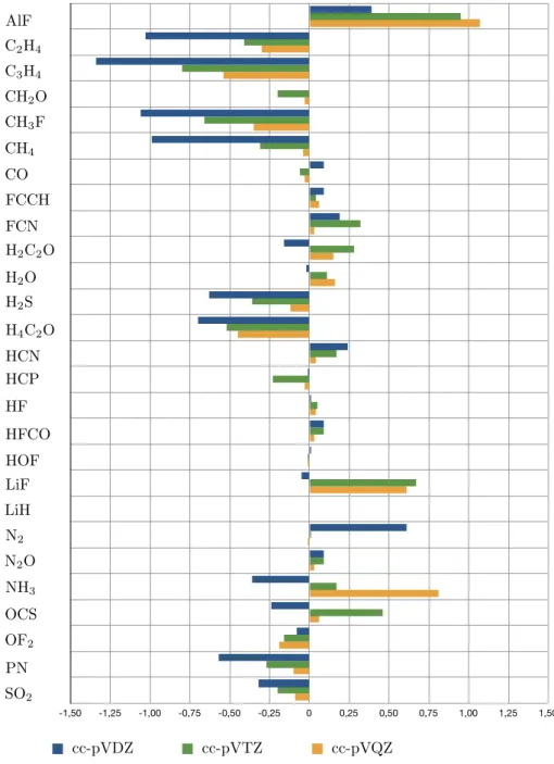
![Figure 3.1: Deviation of calculated shieldings (cc-pVQZ basis set) at the levels of GIAO-DF-HF and GIAO-DF-LMP2 from experimental 13 C gas-phase shieldings [85]](https://thumb-eu.123doks.com/thumbv2/1library_info/4648289.1608159/63.892.162.723.225.348/figure-deviation-calculated-shieldings-basis-levels-experimental-shieldings.webp)

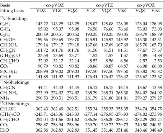


![Table 4.3: Deviation of isotropic magnetizabilities calculated at the levels of HF, LMP2, and LMP2 with full domains and full lists (LMP2 full) from CCSD(T) / aug-cc-pCV[TQ]Z benchmark values [45]](https://thumb-eu.123doks.com/thumbv2/1library_info/4648289.1608159/114.892.186.705.406.757/table-deviation-isotropic-magnetizabilities-calculated-levels-domains-benchmark.webp)