Radiometric approach for the detection of

Radiometric approach for the detection of

picophytoplankton assemblages across oceanic fronts

P

K

L

,

P. J

W

,

Z

K. E

,

G

D

’O

,

R

J.

W. B

,

M

V. Z

,

G

A. T

,

H

A. B

,

W

H. S

,

S

E. C

,

N

J.

P

,

A

B

,

M

W. L

,

I

C

1Ocean Ecology Laboratory, NASA Goddard Space Flight Center, Greenbelt, MD 21077, USA

2Universities Space Research Association, 7178 Columbia Gateway Drive, Columbia, MD 21046, USA

3Blue Marble Space Institute of Science, Seattle, WA 98154, USA

4NASA Postdoctoral Program Fellow, Ocean Ecology Laboratory, NASA Goddard Space Flight Center, Greenbelt, MD 21077, USA

5National Centre for Earth Observation, Plymouth Marine Laboratory, Plymouth PL1 3DH, UK

6College of Life and Environmental Sciences, University of Exeter, Penryn, Cornwall TR10 9EZ, UK

7Scottish Association for Marine Science, Scottish Marine Institute, Dunbeg, Oban, Argyll, PA37 1QA Scotland, UK

8Department of Earth Sciences, University of Oxford, South Parks Rd, Oxford OX1 3AN, UK

9Sequoia Scientific, Inc., 2700 Richards Road, Suite 107, Bellevue, WA 98005, USA

10Bigelow Laboratory for Ocean Sciences, 60 Bigelow Drive, East Boothbay, ME 04544, USA

11Climate Sciences, Alfred-Wegener-Institute Helmholtz Center for Polar and Marine Research, D-27570 Bremerhaven, Germany

12Institute of Environmental Physics, Department of Physics and Electrical Engineering, University of Bremen, D-28359 Bremen, Germany

*priscila@bmsis.org

Abstract: Cell abundances ofProchlorococcus,Synechococcus, and autotrophic picoeukaryotes were estimated in surface waters using principal component analysis (PCA) of hyperspectral and multispectral remote-sensing reflectance data. This involved the development of models that employed multilinear correlations between cell abundances across the Atlantic Ocean and a combination of PCA scores and sea surface temperatures. The models retrieve high Prochlorococcusabundances in the Equatorial Convergence Zone and show their numerical dominance in oceanic gyres, with decreases inProchlorococcusabundances towards temperate waters whereSynechococcusflourishes, and an emergence of picoeukaryotes in temperate waters.

Fine-scalein-situsampling across ocean fronts provided a large dynamic range of measurements for the training dataset, which resulted in the successful detection of fine-scaleSynechococcus patches. Satellite implementation of the models showed good performance (R²>0.50) when validated against in-situdata from six Atlantic Meridional Transect cruises. The improved relative performance of the hyperspectral models highlights the importance of future high spectral resolution satellite instruments, such as the NASA PACE mission’s Ocean Color Instrument, to extend our spatiotemporal knowledge about ecologically relevant phytoplankton assemblages.

Published by The Optical Society under the terms of theCreative Commons Attribution 4.0 License. Further distribution of this work must maintain attribution to the author(s) and the published article’s title, journal citation, and DOI.

#398127 https://doi.org/10.1364/OE.398127

Journal © 2020 Received 20 May 2020; revised 31 Jul 2020; accepted 3 Aug 2020; published 17 Aug 2020

1. Introduction

Observing spatiotemporal changes in the composition of phytoplankton assemblages over broad areas of the ocean increases our understanding of the response of these critical photoautotrophs to environmental and climatic processes. The smallest phytoplankton cells, most often categorized as picophytoplankton (<2 µm [1]) or ultraphytoplankton (<3 µm [2]), are the most abundant primary producers in the global ocean. Despite their individually low biomass relative to other primary producers [3,4], picophytoplankton are dominant in∼50% of the world’s surface oceans, where the reduced availability of inorganic nutrients limits the growth of larger phytoplankton cells [5–7]. Composed of the cyanobacteriaProchlorococcus(∼0.8 µm) andSynechococcus (∼1 µm), as well as a polyphyletic group of picoeukaryotes, picophytoplankton are responsible for 50 to 90% of all primary production in open ocean ecosystems [8,9]. They therefore play a substantial role in the maintenance of the marine food web and contribute up to 30% of the total carbon export to the deep ocean [10–12].

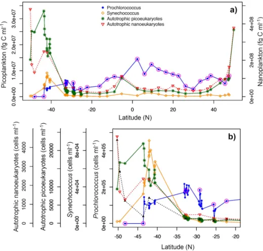
Given the important ecological and biogeochemical roles of picophytoplankton, the oceano- graphic community invests substantially in improving our scientific understanding of their spatiotemporal patterns. Ship-basedin-situmeasurements of phytoplankton composition have revealed important paradigms in their diversity [13–18]. In the Atlantic Ocean, for example, Prochlorococcusinhabits warmer and mostly oligotrophic waters surrounded by spatially adjacent fronts of sub-mesoscaleSynechococcuspatches [8,13,18]. These fronts often reside at boundaries where phytoplankton communities start to transition to higher concentrations of larger eukaryotic cells, such as picoeukaryotes and nanoeukaryotic flagellates [8,19] (Fig.1). Hence, identification ofProchlorococcusandSynechococcusdistributions may conceptually be used to identify trophic boundaries in oceanic ecosystems [20], in addition to providing insight into productivity, food web regimes, and carbon export.

Ocean color satellite instruments provide a tool for capturing and retrospectively analyzing phytoplankton spatiotemporal patterns on synoptic and long-term scales that are unattainable by conventionalin-situmethods [21–23]. These instruments measure visible and near-infrared radiances at discrete wavelengths at the top-of-the atmosphere. Atmospheric correction algorithms are applied to remove contributions of the atmosphere and surface reflection from the total signal, leaving estimates of spectral remote-sensing reflectances (Rrs(λ); sr⁻¹), the light exiting the water column normalized to the downwelling surface irradiance [24]. Bio-optical algorithms are subsequently applied to theRrs(λ) to produce estimates of near-surface concentrations of the photosynthetic pigment chlorophyll-a (Chl; mg m⁻³) and other metrics of phytoplankton community composition [25–27]. Other existing bio-optical algorithms provide abundances or biomass of different phytoplankton using unique empirical relationships between cell abundance andRrs(λ), as well as additional satellite observables such as sea surface temperature (SST; °C) and photosynthetically active radiation (PAR; µE m⁻²s⁻¹) [9,28–30].

To date, the majority of bio-optical algorithms that explore phytoplankton community compo- sition exploit the capabilities of multispectral ocean color satellites, using only a few wavelengths of anRrs(λ) spectrum [21,23,31]. More recent approaches consider increased spectral resolution, following the development of commercial off-the-shelf instrumentation allowing the hyperspec- tralin-situmeasurement ofRrs(λ) and the expectation that hyperspectral ocean color satellite instruments will be launched in the foreseeable future [32]. Given the higher information content of hyperspectral radiometry, sophisticated statistical methods have been successfully applied to assess its variability and correlation with phytoplankton attributes of interest [18,33–39]. The forthcoming NASA Plankton, Aerosol, Cloud, ocean Ecosystem (PACE) mission is expected to increase the interest and demand for hyperspectral methods for global phytoplankton community composition assessment [40].

In this paper, we present empirical algorithms based on principal component regressions that provide estimates of surface abundances ofProchlorococcus,Synechococcus, and autotrophic

Fig. 1. a)Carbon concentration estimated from flow-cytometric cell counts across the Atlantic Meridional Transect, andb)cell abundance (scaled to group-specific maximum cell abundance) ofProchlorococcus(blue),Synechococcus(orange), autotrophic picoeukaryotes (green) and autotrophic nanoeukaryotes (red) in surface waters of the frontal system between the South Atlantic Gyre and temperate waters of the South Atlantic (subset of the southern portion of the transect in (a)). Data collected during AMT24 (2014). Red circles in Prochlorococcusindicate samples that were taken from CTD casts. The remaining samples (across theSynechococcusfront) were taken from the ship’s underway system.

picoeukaryotes, derived fromin-situdatasets of measured cell abundances and hyperspectral Rrs(λ). First, we explore the viability of principal component techniques for the identification of some of the smallest phytoplankton community members using hyperspectral and multispectral Rrs(λ). This exploration includes an assessment of performance enhancement using both Rrs(λ) and remotely sensedSSTas an additional predictor. Second, we evaluate the relative performance of multi- and hyperspectral implementations of these algorithms. These comparisons quantify improvements inProchlorococcusandSynechococcusretrievals when additional spectral information is used. Knowledge of such performance differences provides a metric of relative uncertainty to be considered when evaluating results from heritage multispectral satellite instruments in comparison with forthcoming hyperspectral satellite instruments such as NASA’s PACE mission [40].

2. Material and methods

2.1. Algorithm training in-situ dataset

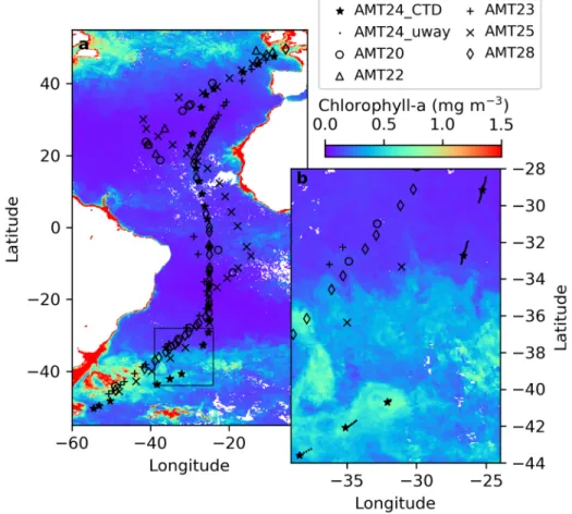
Radiometric, hydrographic, and phytoplankton abundancein-situdata for algorithm training were collected during the Atlantic Meridional Transect 24 (AMT24) oceanographic expedition, which took place between the United Kingdom and the Falkland Islands during boreal autumn (September 30^thto November 1^st, 2014) onboard the RRS James Clark Ross. AMT24 covered most biogeochemical provinces of the Atlantic Ocean (Fig.2), capturing several marine ecosystems inclusive of ocean gyres, the highly productive Equatorial Convergence Zone, and the high-latitude boundaries of the ocean gyres [8,41].

Fig. 2.a)CTD stations for the training dataset (Atlantic Meridional Transect 24 - AMT24), and the validation datasets (AMTs 20, 22, 23, 25 and 28), with the monthly composite of chlorophyll (MODerate resolution Imaging Spectroradiometer onboard Aqua - Aqua- MODIS) in October/2014, andb)magnification of frontal region between the South Atlantic Gyre and temperate waters, highlighting the frequent underway samples (dots).

The sampling strategy to generate an appropriate dataset to develop a predictive algorithm targeted to a phytoplankton group must be designed according to the spatial scales of variability for this group. As such, consideration of previous knowledge about the biology and ecology of this phytoplankton group is useful. With that in mind, we considered two different approaches to collect discrete samples for the analysis of picophytoplankton community structure. First, daily surface (<10 m depth) samples were collected at 13:00 (local time) using a Niskin bottle deployed

as part of the CTD rosette (Fig.2). Second, additional surface samples were collected every 30 minutes from the underway system of the ship (Fig.2) while crossing the front between the South Atlantic Gyre and temperate waters (latitude from 25°S to 45°S). This is the region where we expect a transition fromProchlorococcusdominance into the sub-mesoscaleSynechococcus patches. Water temperature was measured using a CTD (Sea-Bird Electronics SBE 9/11) installed on the rosette profiler or using the hull-mounted shipboard CTD unit (SBE 3P). More details on the underway sampling can be found in Brewin et al. [42].

Above-water radiometric data were collected in continuous underway mode using three Sea-Bird Electronics HyperSAS radiometer systems (measuring total upwelling radianceLt(λ), sky radianceLsky(λ), and planar downwelling irradianceEd(λ)) as described by Brewin et al. [43].

The radiometers have nominal spectral resolution of 10 nm and spectral sampling of 3.3 nm. The procedure to process radiometric data followed protocols described in the same reference, with the following modifications: 1) raw radiometric data were converted to physical quantities using calibration coefficients computed as the average between the pre- and post-cruise calibrations; 2) corrections for dark counts, interpolated in time and over a common wavelength range, were done as in Brewin et al. [43]; 3) continuous measurements of pitch and roll were used to compute tilt angles and all radiometric measurements corresponding to tilt angles≥5°, or with solar zenith angles≥80° and≤10° were discarded; 4) the relative azimuth angle (∆φ) between sensor (φ) and sun (φ₀) was computed as∆φ=φ–φ₀and all radiometric measurements with∆φ≥170°

and∆φ≤50° were discarded; and, 5) an existing technique based on the assumed absence of upward radiance in the near infrared in open-ocean waters [44] was adapted to minimize sun glint. For the latter, we divided the continuous underway dataset into 1-minute intervals and for each interval we only retained the data corresponding to theLt(λ) spectrum that had the minimum Lt(λ) in the near-infrared spectral region as determined by the average of values in the 750-800 nm range. Water-leaving radiance (Lw(λ)) was computed by subtracting the influence of sky and sunlight specularly reflected by the sea surface using the following equation:

Lw=Lt−ρ_skyLsky−LNIR, (1) whereρ_skyandLNIRare scalar coefficients that we obtained by minimizing the following cost function:

C=Õ_λ=800

λ=750|Lt(λ) −ρ_skyLsky(λ) −LNIR|. (2)

In practice, this minimization routine ensures that the derivedLw(λ)is approximately zero and spectrally flat between 750 and 800 nm. Finally, remote-sensing reflectances were computed by dividingLw(λ) byEd(λ).

Once processed,R_rs(λ) from 414 to 660 nm were interpolated (2 nm resolution), then quality- controlled by removing: 1) measurements collected earlier than 09:00 local time or later than 17:00 local time; 2) spectra that showed negative values in the visible range (400-700 nm); and, 3) spectra with second derivative values higher than 2×10⁻⁴sr⁻¹nm⁻¹or lower than -2×10⁻⁴ sr⁻¹nm⁻¹in the spectral region from 610 to 660 nm, as a means of noise removal. Coincidence between in-situRrs(λ) measurements and discrete sampling locations was determined by time (date, hour, and minute of sampling). Prior to the numerical analysis, eachRrs(λ) spectrum was standardized (Rrs’(λ)) [33,35] following:

Rrs0(λ=i)= R_rs(λ=i) − mean[R_rs]⁶⁶⁰

414

sd[Rrs]⁶⁶⁰

414

, (3)

whereRrs(λ=i) is theRrsat thei^th wavelength, andmeanandsd[Rrs]⁶⁶⁰₄₁₄ are the average and standard deviations ofRrs(λ)of values between 414 and 660 nm in oneRrs(λ)spectrum. This standardization of theRrs(λ) curves highlights spectral features ofRrs(λ) and minimizes variance

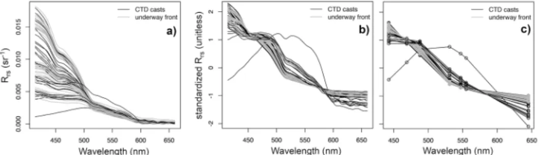
due to amplitude. Within open ocean (case 1) waters, the variability in the shapes of spectral features are mostly governed by phytoplankton absorption properties (i.e., pigments and packaging) [45], which provide the most useful spectral characteristics to differentiate between taxonomic groups. Features caused by changes in the spectral slope of backscattering and absorption by colored dissolved organic matter (CDOM) are still reflected in the shape of standardizedRrs’(λ) spectra. Less spectrally distinct changes inRrs(λ) result from backscattering effects driven by particle morphological characteristics and refractive indices, and from processing errors in underway measuredRrs(λ) such as sea-surface correction and cloud effects. The measuredRrs’(λ) spectra from the AMT24 dataset are shown in Fig.3.

Fig. 3. Remote-sensing reflectances (Rrs(λ)) measured at discrete sampling locations across the Atlantic Ocean during AMT24: a)original hyperspectral measurements; b) standardized hyperspectral measurements;c)standardized multiband measurements at the central wavelengths of seven Aqua-MODIS bands: 443, 469, 488, 531, 547, 555, and 645 nm.

Picophytoplankton cell concentrations (cells ml⁻¹) were analyzed in 1.6 ml seawater samples preserved with paraformaldehyde using a FACSCalibur (Becton Dickinson) flow cytometer.

Yellow-green 0.5 and 1.0µm reference beads (Fluoresbrite Microparticles, Polysciences, War- rington, PA, USA) were used as an internal standard for both fluorescence and flow rates [46].

ForProchlorococcusandSynechococcus, samples were stained with a 1% commercial stock solution of SYBR Green 1 (Molecular Probes, Inc.) in Milli-Q water, then mixed with 300 mol m⁻³tripotassium citrate (24.5 mol m⁻³final concentration) [47]. This method allows the distinction of different populations of microbes based on their DNA content and right-angle light scatter (RALS), regardless of their intracellularChlcontent (red fluorescence) [46]. Autotrophic eukaryotes were quantified based on their red fluorescence andRALS, using the method described in Olson et al. [48]. The AMT24 picoplankton dataset is freely available [49].

2.2. Validation in-situ datasets

Radiometric, hydrographic, and phytoplankton abundancein-situdata for algorithm validation were collected during several oceanographic expeditions. First, cross-validation (see section2.4) was performed using the same AMT24 dataset that was used for training the model. Then, a satellite implementation was tested using flow cytometric counts from five additional AMT cruises (AMT20, 22, 23, 25, and 28) [50–53] and coincidentRrs(λ) andSSTsatellite retrievals (see details in section2.3), provided by the British Oceanographic Data Centre (BODC) [52]. Flow cytometric quantification ofProchlorococcus,Synechococcusand autotrophic picoeukaryotes was conducted using the method described in Olson et al. [48], except on AMTs 23 and 25 where Prochlorococcuswas quantified following Zubkov et al. [47]. The collection and processing of flow cytometric data on these cruises followed the methods described in Lange et al. [28]. The five AMT cruises surveyed similar locations and occurred in similar seasons (late September

to early November) spanning 2010 to 2018 (detailed information on cruise tracks and dates are described in the Atlantic Meridional Transect website [54]).

2.3. Satellite data

MODerate resolution Imaging Spectroradiometer onboard Aqua (Aqua-MODIS) data were acquired from the NASA Ocean Biology Processing Group [55]. This included Level-3, 4-km global maps ofRrs(λ) andSSTspanning the following periods: daily and 8-day composites from September 30^thto November 1^st, 2014 (the duration of AMT24); and 8-day composites spanning October 12^thto November 25^th2010 (AMT20), October 10^thto November 24^th2012 (AMT22), October 3^rdto November 4^th2013 (AMT23), September 11^thto November 4^th2015 (AMT25) and September 23^rdto October 30^th2018 (AMT28). Data from 8-day satellite composites were considered to matchin-situsampling locations when the date of thein-situcollection fell within the 8-day window of the composite and its location was located inside a valid 4-km satellite pixel.

The October 2014 monthly cell abundance composites were created by averaging products that used 8-day composites from October 2014 as input.

Although the temporal interval between in-situ and satellite data may be long (for instance 3-4 days) when using 8-day satellite composites, the abundance of picophytoplankton cells are not expected to change abruptly over time in stratified environments where they are most abundant (i.e. ocean gyres and Equatorial divergence zone). Phytoplankton community structure in these regions gradually changes over the seasons, with a much less dynamic behavior than temperate waters and shelf seas. Thus, these operationally-viable retrievals from 8-day satellite composites show their distribution patterns in enough detail and an acceptable associated uncertainty led by temporal mismatch. Data processing and quality assurance followed the OBPG reprocessing configuration 2018.0 [55]. Available visible Aqua-MODISRrs(λ) from the OBPG were used at 443, 469, 488, 531, 547, 555, and 645 nm wavelengths. SatelliteR_rs(λ) spectra were standardized according to Eq. (3) before being utilized for model implementation.

2.4. Model development

Following Craig et al. [33] and Bracher et al. [35], we used principal component regression to derive empirical relationships for the prediction of the abundances of Prochlorococcus, Synechococcus and autotrophic picoeukaryotic cells from scores of a principal component analysis (PCA) ofin-situ Rrs’(λ) from AMT24. We also considered theSSTmeasured in the AMT24 stations as an additional predictor to improve the performance of the PCA score-based empirical models. The decomposition of standardizedRrs(λ) spectra via PCA was performed in R using the functionprcomp(package stats [56]), using: 1) hyperspectralRrs’(λ) spanning 414-660 nm with 2 nm intervals, hereafter referred to as PCAh, and 2)Rrs(λ) measurements at the seven Aqua-MODIS wavelengths (443, 469, 488, 531, 547, 555, 645 nm) available in the HyperSAS measurement range, hereafter referred to as PCAm. The matrixXwith theRrs’(λ) spectra was decomposed into principal components (PC) via:

X(n,w)=U(n,p) Õ

(p)V(w,p)^T, (4)

where the matrixVof loadings (also known as eigenvectors) shows the spectral contributions to each PC (or mode), the vectorÍ

contains the singular values (square-root of scores), and the matrixUof scores (or eigenvalues) consists of the projection of samples at each PC driven by the variability ofRrs’(λ) in distinct sections of the spectrum [35]. The valuesn,w, andpin parentheses indicate dimensions of the matrices and correspond to the number of observations, number of wavelengths, and number of PCs, respectively, where the number of PCs is equal to the smallest number betweennandw. Derived PCs with a standard deviation lower than 0.1% of the standard deviation of the first PC were discarded, resulting in 20 PCs from PCAh and 5 PCs

from PCAm. Additional PCs were discarded based on their significance as a predicting variable in the empirical model (p-values>0.05), resulting in 14 PCs for PCAh and 3 PCs for PCAm.

The PC scores were used as predictors in multilinear regression analyses targeting the abundances ofProchlorococcus(Pro) (Eq. (5)),Synechococcus(Syn) (Eq. (6)), and autotrophic picoeukaryotes (Apeuk) (Eq. (7)). The initial empirical models were developed usingSSTand all PC scores as predictors. Irrelevant predictors (highest p-value in the regression model) were then systematically discarded using backward stepwise selection. As each predictor was discarded, the new model (without the discarded predictor) was compared with the previous model (including that predictor) using the Akaike Information Criteria (AIC), and the model with the lower AIC value was selected. This process was interrupted when the model that included a target predictor showed lower AIC than the model where it was removed. Then, the other variables were removed one by one, and the AIC was re-calculated to assure the best selection of variables, including those with low p-values in the regression. In the final regressions,SSTwas used as an additional predictor forProchlorococcusand picoeukaryotes, composing the following formulations:

yPro = a+ b0log₁₀(SST) +b1u1+b2u2+. . .+bpup (5)

log₁₀(ySyn) = a+ b1u1+b2u2+. . .+bpup, and (6)

log₁₀(yApeuk) = a+ b0log₁₀(SST) +b1u1+b2u2+. . .+bpup (7) whereyis the concentration of cells (cells ml⁻¹),u1,2,...,pis the score of aRrs’(λ) spectrum in thep^th PC from the matrixU,ais the intercept, andb0,1,2,...,pare the regression coefficients.

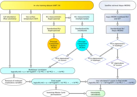
The explanatory variableSSTand the response variables (cell abundances ofSynechococcus and autotrophic picoeukaryotes) were log-transformed for the multilinear regression analysis to achieve a normal distribution. In contrast, cell abundances ofProchlorococcusdemonstrated normal distribution, thus log-transformation was not required and, when implemented for testing, significantly reduced the performance of the empirical model. The workflow of calculations is displayed in Fig.4.

2.5. Model uncertainty assessment

To assess the robustness of the empirical models, cell abundance estimates were compared with thein-situobservations using the approach proposed by Seegers et al. [57], which includes two statistical metrics for uncertainty: average bias (Eq. (8)) and mean absolute error (MAE, Eq. (9)), assuming the normal frequency distribution of the variables. Here, we also calculate the adjusted coefficient of determination (R², Eq. (10)). These metrics were calculated as follows:

bias=10ˆ 1

n Õ_n

i=1 log10(X_i^P) − log10(X_i^O)

, (8)

MAE = 10ˆ 1

n Õ_n

i=1|log10(X_i^P) − log10(X_i^O) |

, and (9)

R² = 1− (1−R²)

n −1 n − (k+1)

(10) wherenis the number of observations,X^Pis the predicted variable,X°is the observed variable, andk is the number of independent variables in the equation. For consistency across all phytoplankton assemblages, all metrics were calculated in logarithmic space, and reported values therefore can be assessed as relative or percentage uncertainties (i.e., Eqs. (3) and (4) from Seegers et al. [57]). Uncertainties were calculated using the following dataset arrangements:

1) Full-fit in-situ predictions: Models trained with the AMT24 dataset were used to compute cell abundances fromin-situ Rrs(λ) measurements from AMT24 and predictions were compared toin-situobservations of cell abundances from AMT24, which were also used for developing the models (Tables1and2);

2) Cross-validation based on in-situ predictions: Models trained with randomly sub-sampled training datasets (80% of the original AMT24 dataset) were used to compute cell abundances using the remaining 20% of the dataset, and these predictions were compared with observations from this 20% sub-dataset (bootstrap method). This process was repeated (2000 Monte-Carlo permutations) and the average performance metrics were computed (Tables1and2);

3) Satellite predictions using full-fit multispectral in-situ models: Models trained with the AMT24 dataset were used to compute cell abundances from Aqua-MODISRrs(λ) andSST retrievals (daily and 8-day composites) matching the time and location of sampling of AMT24, and predictions were compared toin-situobservations of cell abundances which were used to develop the prediction models (Table3); and,

4) Validation of satellite predictions with independent datasets: Models trained with the AMT24 dataset were used to compute cell abundances from Aqua-MODISRrs(λ) and SST retrievals (8-day composites) matching the time and location of sampling of five AMT cruises (AMTs 20, 22, 23, 25 and 28), and predictions were compared toin-situ observations of cell abundances (Table3).

Arrangements 1 and 2 assess model performance and robustness against the selection of input data, respectively. Arrangement 2 (cross-validation) allows an assessment of whether or not the

Fig. 4.Workflow of calculations performed in the predictive models: Model design (yellow and blue) and model application to Aqua-MODIS data (grey).

full-fit model is overtrained (i.e., not generalizable to datasets other than its training dataset). If the full-fit and the cross-validation performance metrics show similar results, the model is robust (i.e., not overtrained). Arrangements 3 and 4 are used to assess the performance of the model in terms of application to satellite data to assess its uncertainty by validation with independent datasets. All statistical analyses were performed using the R packagesstats[56],MASS[58], and devtools[59].

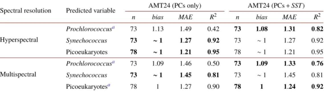
Table 1. Arrangement 1 uncertainty calculations for cell abundance (cells ml⁻¹) model estimates of Prochlorococcus,Synechococcusand autotrophic picoeukaryotes during AMT24, with or without

SST. Bias and MAE were calculated in log₁₀normal space, thus are expressed in relative values corresponding to the percentage deviation from 1 (i.e., 1.09= +9%, 0.93=–7%) . R²was calculated in

log₁₀normal space forSynechococcusand picoeukaryotes, but with untransformed data for ProchlorococcusbecauseProchlorococcusabundances naturally show a normal distribution. The

best performing hyperspectral and multispectral models using either PCs+SST or PCs only are indicated in bold, with corresponding results shown in Fig. 6.

Spectral resolution Predicted variable AMT24 (PCs only) AMT24 (PCs+SST)

n bias MAE R² n bias MAE R²

Hyperspectral

Prochlorococcus^a 73 1.13 1.49 0.42 73 1.08 1.31 0.82

Synechococcus 73 ∼1 1.27 0.92 73 ∼1 1.27 0.92

Picoeukaryotes 78 ∼1 1.21 0.95 78 ∼1 1.21 0.95

Multispectral

Prochlorococcus^a 73 1.09 1.46 0.50 73 1.09 1.33 0.76

Synechococcus 73 ∼1 1.45 0.81 73 ∼1 1.45 0.81

Picoeukaryotes^a 78 1 1.27 0.90 78 1 1.24 0.92

aModels chosen to use sea surface temperature (SST) as an additional predictor.

Table 2. Arrangement 1 (full-fit) versus 2 (cross-validation) uncertainty calculations for cell abundance model estimates ofProchlorococcus,Synechococcusand autotrophic picoeukaryotes during AMT24. Bias and MAE were calculated in log₁₀space, thus are expressed in relative values corresponding to the percentage deviation from 1 (i.e., 1.09= +9%, 0.93=–7%). R²was calculated in

log₁₀space forSynechococcusand picoeukaryotes, but with untransformed data for ProchlorococcusbecauseProchlorococcusabundances naturally show a normal distribution.

Spectral resolution Predicted variable All AMT24 (Arrangement 1) Re-sampled AMT24 (Arrangement 2)

n bias MAE R² n bias MAE R²

Hyperspectral

Prochlorococcus^a 73 1.08 1.31 0.82 16 1.08 1.35 0.78

Synechococcus 73 ∼1 1.27 0.92 16 ∼1 1.36 0.85

Picoeukaryotes 78 ∼1 1.21 0.95 16 ∼1 1.26 0.92

Multispectral

Prochlorococcus^a 73 1.09 1.33 0.76 16 1.11 1.38 0.74

Synechococcus 73 ∼1 1.45 0.81 16 1.01 1.50 0.74

Picoeukaryotes^a 78 1 1.24 0.92 16 0.94 1.39 0.76

aModels using sea surface temperature (SST) as an additional predictor.

Table 3. Arrangements 3 and 4 uncertainty calculations for cell abundance model estimates (cells ml⁻¹) ofProchlorococcus,Synechococcusand autotrophic picoeukaryotes using Aqua-MODIS R_rs(λ) 8-day-composite retrievals for time and location of AMT24 sampling sites and those of AMTs

20, 22, 23, 25 and 28. Bias and MAE were calculated in log₁₀normal space, thus are expressed in relative values corresponding to the percentage deviation from 1 (i.e., 1.09= +9%, 0.93=–7%). R²

was calculated in log₁₀normal space forSynechococcusand picoeukaryotes, but with untransformed data forProchlorococcusbecauseProchlorococcusabundances naturally show a

normal distribution.

Spectral resolution Predicted variable

AMT24 Aqua-MODIS (8-day composites)

AMTs 20,22-25, 28 Aqua-MODIS (8-day)

n bias MAE R² n bias MAE R²

Multispectral

Prochlorococcus^a 60 1.09 1.37 0.58 113 1.75 2.26 0.54

Synechococcus 68 0.62 2.04 0.50 120 0.93 2.20 0.40

Picoeukaryotes^a 65 0.91 1.28 0.92 120 1.05 1.53 0.60

aModels using sea surface temperature (SST) as an additional predictor.

3. Results

3.1. Selection of explanatory variables

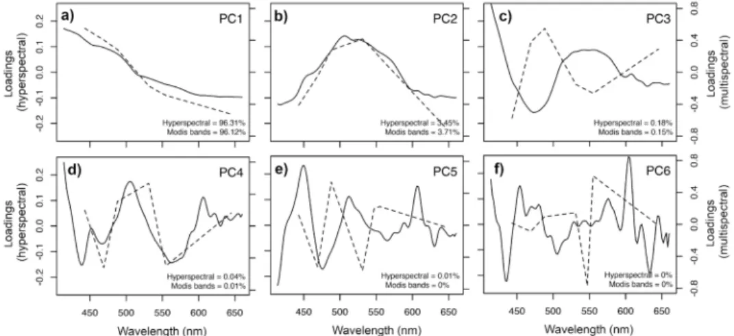
The backward selection of explanatory variables resulted in 14 PCs for PCAh and 3 PCs for PCAm. The loadings of the first 6 PCs for the PCAh and PCAm datasets are shown in Fig.5.

The spectral distribution of PC loadings is akin to results from prior similar approaches [33–35], indicating spectral features related to the optical properties of the seawater constituents. The spectral variability of the first PC is driven mainly by the particulate backscattering of the in-water constituents and the absorption of water molecules, and explained more than 96% of the data covariance for both multi- and hyperspectralRrs’(λ) datasets. The second PC highlights spectral features related to the absorption byChlat the ocean surface, explaining∼3.5% of the dataset covariance; and the third PC is driven by the spectral variation ofRrs’(λ) due to the absorption of accessory pigments and explained∼0.16% of the dataset covariance [33–35]. These first three PCs were similar between hyperspectral and multispectral models, indicating that the most significantR_rs’(λ) features were captured by multispectral data (Fig.5).

In the multispectral models, PCs 1 and 2 were strong predictors for all targeted picophy- toplankton taxa, whereas PC3 was utilized to predict the abundance ofSynechococcusand picoeukaryotes. For the hyperspectral models, the prediction ofProchlorococcusutilized PCs 1 and 2 combined with two other PCs,Synechococcuswas associated with PCs 1, 2 and 3 in association with seven other PCs, and picoeukaryotes were predicted using PCs 2 and 3 with five additional PCs. In addition to using the PCs’ scores as predictors,SSTwas included as a predicting variable and the improvement of the models was evaluated.

3.2. Model performance assessed with the training dataset 3.2.1. SSTas an additional predictor

Regardless of differences in performance metrics, both hyperspectral and multispectral models are capable of detecting the changes in cell concentrations along the AMT 24 transect. However, hyperspectral based models were superior to multispectral ones regardless of the targeted picophytoplankton group (Table1). In addition, for Arrangement 1 (section2.4), the inclusion ofSST as a predictor considerably improved the performance of both the multispectral and hyperspectral models to predictProchlorococcus when compared to models that only used PCs as predictors (Table1). For the hyperspectral approach, theMAE decreased from 1.49 (49%) to 1.31 (31%) andR²increased from 0.42 to 0.82 whenSST was added to the predictive model ofProchlorococcus(Table1, Fig. 6). Likewise, for the multispectral approach, the

Fig. 5.Spectral distribution of loadings of the first six principal components. Solid lines (primary Y axis) show loadings of the PCA using hyperspectralRrs’(λ) (PCAh), whereas dashed lines (secondary Y axis) show those of the PCA usingR_rs’(λ) at the Aqua-MODIS bands (PCAm). Relative (percentage) explanation of the variability of the data by each PC is shown on the bottom right of each plot.

MAEdecreased from 1.46 to 1.33 andR² increased from 0.50 to 0.76 (Table1, Fig.6). The inclusion ofSSTas a predictor did not improve either the multispectral or hyperspectral models to predictSynechococcus, with biases andMAEs remaining unchanged (Table1). For autotrophic picoeukaryotes, uncertainty metrics remained effectively unchanged when consideringSSTfor the hyperspectral approach and, in the multispectral model, theMAEandR²showed an improvement when addingSST(1.27 to 1.24 and 0.90 to 0.92, respectively) (Table1). We opted to useSST as an additional predictor in the models to estimate the abundance ofProchlorococcususing both multi- and hyperspectralRrs’(λ), and in the model to predict the abundance of autotrophic picoeukaryotes using multispectralRrs’(λ).

3.2.2. Multispectralversushyperspectral cross-validation

Model performance improved when using hyperspectralRrs’(λ) compared to consideration of only Aqua-MODIS bands (see Fig.6, Tables1and2). ForSynechococcusabundance estimation, biases were negligible (Table2) while multispectralMAEs exceeded hyperspectralMAEs in both Arrangements 1 (full-fit) and 2 (cross-validation) (1.45 vs. 1.27 and 1.50 vs. 1.36, respectively).

For the prediction ofProchlorococcusand picoeukaryote abundances, the hyperspectral biases andMAEs were also reduced relative to their multispectral counterparts for both Arrangements 1 and 2 (Table2). Finally, theR²for predictingProchlorococcus,Synechococcus,and autotrophic picoeukaryote abundances increased by 6% on average when using hyperspectral approach compared to the multispectral approach. Nevertheless, and despite underperforming relative to the hyperspectral approach, patterns in the latitudinal variability in the abundance of these groups were still reasonably captured by the multispectral approach, usingSSTwhen applicable, across the full dynamic range of cell concentrations for each phytoplankton group (see Fig.6).

3.3. Model implementation using satellite data (Aqua-MODIS) 3.3.1. Satellite retrievals from AMT cruises

Assessment of our multispectral model using 8-day Aqua-MODISRrs’(λ) andSST imagery (September 30^thto October 7^th, 2014) as input yielded reasonable retrievals of cell concentrations

Fig. 6.Performance of developed models (Arrangement 2) fora-c)Prochlorococcus(first row),d-f)Synechococcus(second row) andg-i)autotrophic picoeukaryotes (third row) cell abundance, using PCAm and PCAh approaches. In panelsd-eandg-h, abundances of Synechococcusand picoeukaryotes are plotted in log10 scale as this transformation was implemented for model development. SSTwas used as an additional predictor for both Prochlorococcusmodels and the multispectral picoeukaryotes model since it was found to improve performance (Table1). Regardless of difference in performance metrics, both hyperspectral and multispectralin-situmodels are capable of detecting the changes in cell concentrations along the AMT 24 transect (c,f,i).

when compared toin-situsamples collected during the AMT24 cruise (Table3). TheMAEof 1.37 forProchlorococcus, 2.04 forSynechococcusand 1.28 for picoeukaryotes was higher than the one encountered forin-situ Rrs’(λ) data (Table1), indicating a degradation in performance when moving to the satelliteRrs’(λ). ThebiasinProchlorococcusprediction remained around 1.09 (9%) when using Aqua-MODISRrs(λ), similar to that usingin-situ Rrs’(λ) measurements.

However, increases in thebiasofSynechococcus(0.62 (–38%) from Aqua-MODIS and∼1 (∼

0%) fromin-situ Rrs’(λ)) and picoeukaryote retrievals (0.91 (–9%) from Aqua-MODIS and 1 (0%) fromin-situ Rrs(λ)) were more evident. These underestimations of cell abundances when using satellite data are likely associated with the “patchy” nature of their spatial distribution, further augmented by mismatch betweenin-situ/satellite sampling times and areas (1.6 ml discrete sample vs. 8 days/4 km composites) (Fig.7).

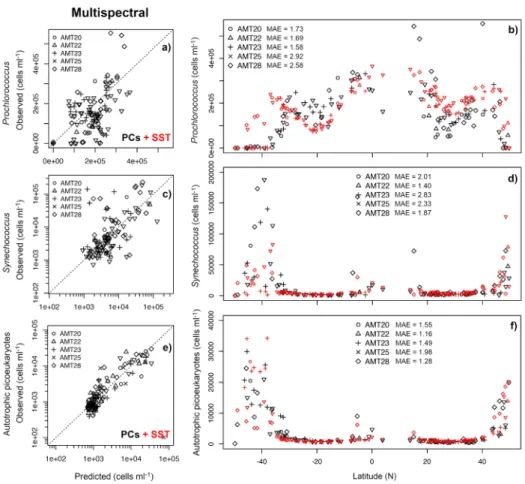
The temporal portability of multispectral models was assessed using cell abundance predictions computed from Aqua-MODIS data retrieved from sampling time/locations of AMTs 20, 22, 23, 25 and 28.Prochlorococcusabundance was overestimated in these 5 AMT cruises, as indicated by the increase inMAE(2.26) and inbias(1.75) when compared to satellite retrievals from AMT24 (MAE=1.37,bias=1.09), especially in the North Atlantic (Fig.8). TheSynechococcus model predictions also showed a higherMAE (2.20) compared to AMT24 (2.04), whereas

Fig. 7.Performance of developed models (PCA_mapproach) fora,b)Prochlorococcus(first row),c,d)Synechococcus(second row) ande,f)autotrophic picoeukaryotes (third row) cell abundance, implemented using Aqua-MODIS retrievals for the cruise AMT24. In panelsc ande, abundances ofSynechococcusand picoeukaryotes are plotted in log₁₀scale because this transformation was implemented for model development.SSTwas used as an additional predictor for models to predictProchlorococcusand autotrophic picoeukaryotes.

Fig. 8. Performance of developed models (PCAmapproach) fora,b)Prochlorococcus (first row),c,d)Synechococcus(second row) ande,f)autotrophic picoeukaryotes (third row) cell abundance, implemented using 8-day Aqua-MODIS retrievals for AMTs 20, 22, 23, 25 and 28. In panelsb,d, andf, black symbols indicatein-situobservations, while red markers indicate values retrieved using species-specific model from Aqua-MODIS, and specificMAEof modelled values from each cruise is shown. In panelscande, abundances ofSynechococcusand picoeukaryotes are shown in log scale, as this transformation was used in model development.SSTwas used as an additional predictor for models to predict Prochlorococcusand autotrophic picoeukaryotes.

picoeukaryotesMAEincreased from 1.28 on AMT24 to 1.53 for the other five AMTs with abias decreasing slightly from 0.91 (– 9%) to 1.05 (5%) (Table3).

3.3.2. Implementation using satellite imagery

The spatial distribution of these picophytoplankton groups captured by our models is shown in Fig.9. Satellite predictions show highest abundances ofProchlorococcusat the Equatorial Convergence Zone and lowest abundances in the ocean gyres (despite still being higher than other phytoplankton), with an increase towards the high-latitude edges of both North and South Atlantic subtropical gyres. Despite the low abundance,Prochlorococcusnumerically dominated the picophytoplankton in the gyres.Synechococcusshowed highest abundances at the high-latitude edges of the ocean gyres. Autotrophic picoeukaryotes were most abundant in higher latitudes (>

45° N and S) showing similar patterns to the distribution ofChl(see Fig.2), with the constraint

ofChlconcentrations being lower than 1 mg m⁻³, since chlorophyll concentrations never reached values higher than this in the present dataset. Satellite visualization of model outputs allowed us to detect the picophytoplankton community zonation at the high-latitude gyre edges (i.e.

Prochlorococcus-Synechococcus-picoeukaryotes from the inner gyres towards higher latitudes), as observed inin-situmeasurements (see Fig.1), demonstrating the potential use of our approach for the evaluation of ecosystem and biogeochemical models.

Fig. 9.Aqua-MODIS monthly composites (October 2014) showing cell abundances (cells ml⁻¹) ofa)Prochlorococcus,b)Synechococcusandc)autotrophic picoeukaryotes at the sea surface.

4. Discussion

Principal component regression analysis provides a powerful tool to retrieve optically-significant marine variables from hyperspectral radiometry by exploring spectral variations in Rrs(λ) [33,35]. With regard to assessing phytoplankton community composition, this method has been implemented most frequently in areas of high phytoplankton biomass, where changes in phytoplankton composition and biomass provide significant changes in phytoplankton absorption that are reflected in spectral variations inRrs(λ) [33,35,60]. The highest picophytoplankton abundances occur in the stable oligotrophic ocean, where the spectral signature of water is influenced not only by the present cells but also by other seawater constituents that co-vary with their abundances such as the absorption of colored dissolved organic matter and backscattering of heterotrophic bacteria, both of which alter the magnitude and shape ofRrs(λ). Considering this, our analysis captures the associations between changes in ocean color and the abundance of the smallest phytoplankton, namelyProchlorococcus,Synechococcus, and autotrophic picoeukaryotes.

In the PCA made withRrs(λ) spectra from the Atlantic Ocean (AMT24) and concurrent cell counts, the first three principal components displayed spectral features directly or indirectly correlated with the abundance of these taxa. For example, PC1 showsRrs(λ) features likely attributed to the backscatter slope and the spectral shape of the absorption of water molecules, having similar shape to the first PC of PCAs from hyperspectralRrs(λ) spectra of meso- and eutrophic waters [33–35]. This first PC was highly correlated with highestProchlorococcus abundances and lowest abundances of larger phytoplankton cells, meaningProchlorococcusis most abundant in waters where the shape of theRrs(λ) spectrum is most similar to that of PC1, thus having lower influence of the absorption ofChl, accessory pigments and other in-water constituents (i.e., oligotrophic waters). PCs 2 to 4 were associated with the presence of accessory pigments and higherChlabsorption, present inSynechococcusand autotrophic picoeukaryotic cells.

Increasing the spectral resolution ofRrs(λ) substantially improved the prediction of all targeted groups (see Tables1and2). HyperspectralRrs(λ) provides greater information content on oceanic constituents contributing to variability in the optical signal, in particular taxon-specific light-absorbing photosynthetic pigments. Pigment-specific light absorption imposes spectral features of several nanometers in distance, leading to variations in the spectral shape ofRrs(λ) signal [23,38]. As a consequence, our hyperspectral approach resulted in a higher number of usable principal components (predictors) than our multispectral approach, ultimately increasing the performance of the hyperspectral predictive models, in particular forSynechococcus. This result agrees with several previous comparisons of hyperspectral and multispectral algorithms that demonstrate how increasing the spectral resolution of theRrs(λ) signal improves predictive models for some phytoplankton taxa [33–35,38].

Remotely-sensed physical ocean properties such asSSTcan be useful to further constrain empirical models that predict algal abundance.SST can be used as a powerful predictor for the accumulation of cells when direct or indirect relationships betweenSSTand certain ecological conditions that favor the target taxon are well known, as previously demonstrated for the prediction of blooms of the harmful dinoflagellateAlexandrium fundyensein the Bay of Fundy [61] and blooms of the diatomPseudo-nitzschiain Chesapeake Bay [62], and in other predicting models for the biomass of specific phytoplankton groups [30,63,64]. In our study, the inclusion ofSST was relevant for predicting the abundances ofProchlorococcusand picoeukaryotes, as ecological niches of both taxa are extremely constrained by temperature [65–67].Prochlorococcusis most abundant in environments with high water column stability [68–70], which is usually associated with highSST [71], whereas picoeukaryotes grow next to the transition between oligo- and mesotrophic waters [41,72], whereSSTis typically slightly lower than at the center of the gyres [73]. The inclusion ofSSTas a predictor was especially useful for improving multispectral models.

The performance of empirical models such as the ones presented here are highly dependent on the training datasets. For example, inclusion of a dataset collected at higher spatial frequency across the frontal region in the South Atlantic allowed for a larger dynamic range in the training dataset, yielding better retrievals for phytoplankton taxa that occur in high-abundance patches such asSynechococcusat the frontal system of the South Atlantic gyre southern boundary [8,29].

When we retrained the multispectral model using only samples collected on CTD casts (sparse sampling strategy),Synechococcuscell abundances were underestimated in these patches as sparse sampling missed small pockets of highSynechococcusabundances, thus not capturing the full range ofSynechococcuscell concentrations. The increased number of samples across theSynechococcuspatch reduced the retrieval biasfrom 0.71 (–29%) to ∼1 (∼0%) when using multispectralRrs(λ) and from 0.84 (–16%) to∼1 (∼0%) when using hyperspectralRrs(λ), whereasMAEwas reduced from 1.67 (67%) to 1.45 (45%) in the multispectral model and from 1.37 (37%) to 1.27 (27%) using the hyperspectral approach. As an empirical model is only good at predicting cell abundances within the cell number range of its training dataset, this result highlights the importance of understanding the scales of cell abundances and its spatial distribution patterns for the targeted phytoplankton taxon when assembling data to train empirical models. Proper design ofin-situ sampling plans must cover the full dynamic range of cell abundances of that particular taxon. Similarly, vertical sampling needs consideration in such analyses given that in situ sampling does not always represent the spectrally-dependent depth range considered in the satellite retrieval. We considered the top 10 m of the water column in these analyses, which does not consider the full euphotic zone in our areas of interest, but does encompass a reasonable fraction of the optically weighted signal observed over the first e-folding depth [74].

Satellite implementation of the empirical models to monthly composites of Aqua-MODIS Rrs(λ) andSSTprovided a qualitative view of the spatial and temporal distributions (see Fig.9)

of targeted taxa, if only to provide a visual case study to assess the portability of our model.

ForProchlorococcus, our model predicts highest surface abundances at the edges of the ocean gyres and Equatorial Convergence, showing similar distribution to that ofin-situobservations from AMT cruises (see Fig.1) [8,14,52]. ThisProchlorococcusdistribution pattern agrees with predictions of other ocean color-based models, such as Alvain et al. [75], El-Hourany et al. [76], and Xi et al. [31], and the model of Lange et al. [28] which combines ocean color information with environmental variables. In turn, a model based solely on environmental variables (SST, photosynthetically-active radiation -PAR) – i.e. Flombaum et al. [29] – estimates highestProchlorococcusabundances in western boundary currents such as the Gulf Stream and the Brazil Current because, in this model,SSTis the most important driver of the distribution ofProchlorococcus. SST is a powerful predictor ofProchlorococcus[65–67], possibly due to its causal relationship with water column stratification [71] which favors the growth of this cyanobacterium [70]. Stratification induces oligotrophy, avoiding the growth of microbial assemblages that include herbivores ofProchlorococcus[77]. The direct relationship between Prochlorococcusand water column stability, rather than temperature, would justify the high Prochlorococcusabundances found in the Mediterranean Sea [78], and its absence in polar regions where stratification is seasonal or episodic. WhileSST may fail to predict the presence ofProchlorococcusin regions where salinity is important in driving stratification, ocean color variables such asRrs(λ) provide direct observation of the surface water components. Rrs(λ) and spectral phytoplankton absorption coefficients (aph(λ)) provide refined information on the presence of optically-relevant phytoplankton, which are abundant in the absence ofProchlorococcus. In other words,Prochlorococcusis most abundant where the optical influence of phytoplankton on theRrs(λ) spectrum is minimal. However, concurrent high abundances ofProchlorococcusand other phytoplankton groups (such as diatoms, nano- and picoeukaryotes) occur in areas where nutrient input is high despite high stratification levels (i.e., highSST), such as the Equatorial Convergence Zone [8,79]. This explains the best performance of ourProchlorococcusmodel when using ocean color information andSSTas predictors.

RegardingSynechococcusestimates, our ocean color-based model finds highest abundances at the high-latitude edges of the ocean gyres, especially the South Atlantic gyre, surrounding possible blooms of larger phytoplankton cells such as coccolithophorids, similar to predictions based onSSTandPAR[29]. Highest abundances of autotrophic picoeukaryotes were found at the higher latitude edges of the ocean gyres (>45° N and S), mimicking patterns seen in theChl distribution. However, picoeukaryotic populations slightly decrease whereChlconcentrations reach values of∼1 mg m⁻³. Such spatial and temporal patterns highlight the importance of these picophytoplankton taxa as proxies for certain ecosystems or trophic conditions. For example, high abundances ofProchlorococcusdelineate the extension of the ocean gyres, and Synechococcusbecomes abundant in a narrow band at the transition between oligotrophic (i.e.

South Atlantic gyre) and mesotrophic waters (i.e. temperate waters of higher latitudes where pico- and nanophytoplankton bloom), as also observed in several studies [8,14,18,41]. It is important to note that our model estimates cell abundances, which are highly correlated with group-specific carbon biomass but not always with pigment concentrations because of photophysiological adaptations of picophytoplankton cells to the different environmental conditions found across oceanic fronts [8,41,80–83].

In a similar way, we hypothesize that the inclusion of datasets from other parts of the ocean outside the Atlantic would improve the global model and allow for basin-specific tuning.

Such models could allow for a segregated assessment of the photophysiological and optical characteristics of basin-specific ecotypes of the picocyanobacteria and picoeukaryotic flora, ultimately improving the performance of these empirical models. Furthermore, the ability of models to retrieve abundances ofSynechococcusand autotrophic picoeukaryotes could be improved by including datasets from coastal and/or highChlareas (>1 mg m⁻³), allowing for

a merged approach (similar to NASA’s current operationalChlalgorithm). In these waters, the contribution ofCDOMand carotenoids in large phytoplankton to the spectral variability of Rrs(λ) is higher, diminishing the relative influence of picophytoplankton cells. However, the spectral characteristics of these two groups are different in complex waters: Synechococcus ecotypes display different concentrations of accessory pigments to adapt to different optical niches [84–87], although they all contain phycobiliprotein complexes which are rather unique and likely to be detected by the PCA; and the taxonomic composition of autotrophic picoeukaryote communities is highly variable according to nutrient availability, temperature and stratification [41,88,89]. This could also deteriorate finding robust models for the specific groups. Xi et al.

[31] used a large global matchup dataset for setting up similar Empirical Orthogonal Function (EOF) models with pigments (measured using HPLC) and satelliteR_rs(λ)data. While eukaryotic phytoplankton groups were very well predicted globally, the prediction skill ofProchlorococcus andSynechococcuswas rather poor.

Observed changes in model performance between ocean basins or different Atlantic cruises may be expected and could stem from multiple sources. First, the occurrence of distinct ecotypes ofProchlorococcusandSynechococcusand combinations of picoeukaryotic taxa in each ocean basin, and their associated optical properties (due to the physiological acclimation and/or evolutionary adaptation) might have made our model specific to the Atlantic Ocean during the AMT sampling season(s) only. Second, the relationships between group-specific cell abundances and theRrs(λ) signature can be influenced by the structure of the ecosystem itself – that is, the presence of other phytoplankton cells (e.g., diatoms in the Equatorial Convergence Zone), or other optically-active water constituents (e.g.,CDOMand non-algal particles). Differences in ecosystem structure, specifically in the top-down control and other loss pathways for these phytoplankton populations, could also potentially influence model predictions. In addition, flow cytometric cell counts enable a precise determination of the abundance of picophytoplankton groups, which can be converted to carbon biomass [81,82], and do not depend on models and their associated uncertainties to attribute group-specific biomass from marker pigments.

However, the use of marker pigments as proxies for phytoplankton taxa is most directly linked to the observed change in theRrs(λ)spectrum, and also provide estimates of the contribution of larger phytoplankton to the total phytoplankton biomass and its influence in theRrs(λ)spectrum, which can be useful for analysis interpretation. Lastly, while methods used to collectRrs(λ) for this study followed similar community-approved procedures, approaches used to quantify the cell abundances on different oceanographic expeditions differ, potentially adding to differing validation performances when comparing outputs of the model with alternate datasets where different flow cytometric procedures were adopted (i.e., Olson et al. [48] versus Zubkov et al.

[47] for quantifyingProchlorococcusandSynechococcus).

Since the goal of the model is to detect the large-scale spatial variability in open ocean waters, where picophytoplankton cells are most abundant, the model has not been tested in shelf seas and coastal waters. We expect that the models will need to be retuned for such waters because the presence of suspended sediments andCDOMwill change the spectral distribution of the eigenvectors of each principal component.

5. Summary and conclusions

Cell abundances ofProchlorococcus, Synechococcus and autotrophic picoeukaryotes were estimated in surface waters of the Atlantic Ocean using empirical models based on a combination ofSSTand the scores of anRrs(λ) principal component analysis, which captured the association between changes in ocean color and the abundance of these picophytoplankton groups. These models were implemented using satellite data (Aqua-MODIS), which allowed us to estimate cell abundances on a basin scale. Although these phytoplankton types occur in high abundances in oligotrophic oceans, the spectral signature of waters inhabited by these cells is highly influenced