Assessment of the Atlantic water layer in the Arctic Ocean in CMIP5 climate models

https://doi.org/10.1007/s00382-019-04870-6

Assessment of the Atlantic water layer in the Arctic Ocean in CMIP5 climate models

Qi Shu^1,2,3  · Qiang Wang⁴  · Jie Su^5,6 · Xiang Li⁷ · Fangli Qiao^1,2,3

Received: 22 January 2019 / Accepted: 18 June 2019 / Published online: 29 June 2019

© The Author(s) 2019

Abstract

Atlantic water (AW) plays an important role in the thermal balance of the Arctic Ocean, but thus far there has been no comprehensive assessment of the AW layer in the Arctic Ocean simulated by coupled climate models in the framework of Coupled Model Intercomparison Project (CMIP). In this study we assessed the climatology and the trend of the Arctic AW layer in the historical simulations of 41 CMIP5 climate models. The results show that the CMIP5 intermodel spread is large in terms of simulated hydrography, AW core temperature (AWCT) and AW core depth (AWCD) in the Arctic Ocean. The CMIP5 multimodel means are found to be able to reproduce the main climatological spatial patterns of both the AWCT, which is warm near the Fram Strait and decreases along the AW pathways, and the AWCD, which deepens along the AW pathways. However, similar to standalone ocean-ice models, the CMIP5 climate models also face the common problems of too deep and too thick AW layer. AWCT bias in the Arctic Ocean is related to simulated water properties near the Fram Strait and in the Kara and Barents seas. Models with large AWCT biases are those with large biases in AW temperature in the Fram Strait. The biases of AWCT are also significantly correlated with the ocean temperature in the Kara Sea, which is modulated by winter cooling, hence the mixed layer depth and sea ice cover in the Barents Sea. The CMIP5 models largely underestimate the interannual variability of the AWCT, and the CMIP5-simulated increasing trend of the AWCT in the Arctic Ocean is considerably lower than the observed one since the late 1970s.

1 Introduction

The Arctic Ocean is connected to the Atlantic Ocean on both sides of Greenland and to the Pacific Ocean through the Ber- ing Strait (Talley et al. 2011). Water exchange between the Atlantic and Arctic oceans is important for both the regional climate and the global thermohaline circulation (Aagaard et al. 1985; Dickson et al. 2008). Understanding the Arctic Ocean changes and predicting its future evolution are among the key topics of climate research.

The main water mass at the Arctic intermediate depth, the Atlantic water (AW), originates from the North Atlan- tic. Warm and saline AW enters the Nordic Seas in the North Atlantic Current, and then travels northward as two branches of the Norwegian Atlantic Current (Orvik and Niiler 2002). Part of the eastern branch enters the Barents Sea, and then flows into the intermediate and deeper layers of the Arctic Ocean at the St. Anna Trough in the north- ern Kara Sea (Schauer et al. 2002a; Karcher and Oberhu- ber 2002; Maslowski et al. 2004). The remaining part of the eastern branch and the western branch approach the Fram Strait as the West Spitsbergen Current (WSC). Part

Electronic supplementary material The online version of this article (https ://doi.org/10.1007/s0038 2-019-04870 -6) contains supplementary material, which is available to authorized users.

* Qi Shu shuqi@fio.org.cn

1 First Institute of Oceanography, Ministry of Natural Resources, Qingdao, China

2 Laboratory for Regional Oceanography and Numerical Modeling, Pilot National Laboratory for Marine Science and Technology (Qingdao), Qingdao, China

3 Key Laboratory of Marine Science and Numerical Modeling, Ministry of Natural Resources, Qingdao, China

4 Alfred Wegener Institute Helmholtz Centre for Polar and Marine Research, Bremerhaven, Germany

5 Physical Oceanography Laboratory/CIMST, Ocean University of China, Qingdao, China

6 Laboratory for Ocean and Climate Dynamics, Pilot National Laboratory for Marine Science and Technology (Qingdao), Qingdao, China

7 Key Laboratory of Ocean Circulation and Waves, Institute of Oceanology, Chinese Academy of Sciences, Qingdao, China

of the WSC enters the Arctic Ocean, supplying the warm AW layer (Rudels and Friedrich 2000; Schauer et al. 2008;

Beszczynska-Moeller et al. 2012), and the remaining part of the WSC recirculates in the Fram Strait and becomes part of the southward flowing East Greenland Current (EGC) (Marnela et al. 2013; Hattermann et al. 2016; Wekerle et al.

2017). The AW circulates mainly cyclonically in the Arc- tic basins and is aligned with the bathymetry (Rudels et al.

1994; Karcher et al. 2003). It plays an important role in the heat budget of the Arctic Ocean. After leaving the Arctic Ocean in the EGC, it supplies the dense waters that feed the Atlantic overturning circulation (Rudels and Friedrich 2000;

Karcher et al. 2011). Although AW is at the intermediate depth and is not directly in contact with the surface Arctic Ocean, a warming trend in the AW layer in the Arctic Ocean has been observed (Polyakov et al. 2012, 2013), with an implication on accelerating sea ice decline in a warming cli- mate (Polyakov et al. 2004, 2010, 2017; Ivanov et al. 2018).

Climate models are useful tools for studying Arctic climate dynamics and predicting future climate changes.

Although the performance of AW layer simulations in forced ocean-ice models has been assessed thoroughly in the Arctic Ocean Intercomparison Project (AOMIP, Proshutinsky and Kowalik 2007; Proshutinsky et al. 2011) and the Coordi- nated Ocean-ice Reference Experiments, phase II project (CORE-II, Griffies et al. 2009) by Holloway et al. (2007) and Ilicak et al. (2016), comprehensive assessment of the AW layer simulated in state-of-the-art climate models, espe- cially its long-term trend, has not been undertaken. Thus, the performance of AW layer simulations in coupled climate models still remains unknown.

Previous studies have shown that ocean general circula- tion models (OGCMs) used in the AOMIP and CORE-II projects commonly produce an AW layer that is too thick and too deep (Holloway et al. 2007; Ilicak et al. 2016). The common problem is believed to be related to the configura- tion of OGCMs, such as model resolution, vertical mixing schemes, and eddy–topography interaction parameterization.

Unlike ocean-ice models forced with atmospheric reanaly- sis fields used in these studies, climate models allow active atmosphere-ice-ocean coupling, which has advantages such as the avoidance of unphysical freshwater fluxes associated with surface salinity restoring (Griffies et al. 2009). How- ever, ocean models in fully coupled systems might have large biases because of uncertainties in atmospheric and land models and biases in the representation of interaction between ocean and atmosphere. Therefore, it is necessary to evaluate AW layer simulations in state-of-the-art climate models to understand their performance.

The Coupled Model Intercomparison Project Phase 5 (CMIP5) constitutes a useful platform for studying climate change and for assessing the performance of state-of-the-art climate models. In this study we focus on the assessment

of the AW layer in the Arctic Ocean in CMIP5 historical simulations, for which observations are available for com- parison. The paper is structured as follows. The data and methodology are introduced in Sect. 2. Section 3 presents the results, and Sect. 4 provides discussions and the derived conclusions.

2 Data and methodology

This study uses monthly ocean potential temperature and salinity output from the historical simulations (1950–2005) of 41 CMIP5 coupled models, which are available from the Earth System Grid Federation (ESGF) (http://pcmdi 9.llnl.

gov/esgf-web-fe/). There are different ensemble realizations in the different CMIP5 models, and for simplicity, the first ensemble member from each model is selected in this study.

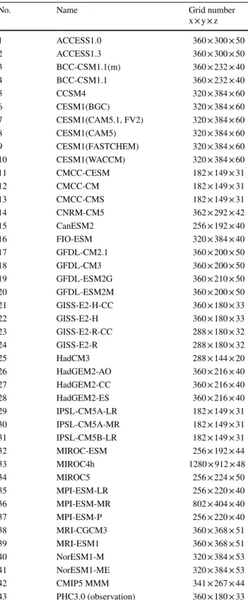
Table 1 lists the names and resolutions of each model used in this study. The horizontal resolution of most models is nomi- nally 1°. The mean horizontal grid numbers of the 41 models are 341 × 267. The MIROC4h model (Sakamoto et al. 2012) has the highest horizontal resolution with 1280 × 912 grid numbers.

Gridded climatological ocean temperature from the Polar Hydrographic Climatology version 3.0 dataset (PHC3.0, Steele et al. 2001) is used as observational reference in this study. The PHC3.0 dataset has high quality in the Arctic Ocean because it is the combination of the World Ocean Atlas, Arctic Ocean Atlas, and some Canadian observations.

In the Arctic Ocean, it mainly covers the period after 1950.

Its horizontal resolution is 1° × 1°. To assess the long-term trend of AW temperature, the time series of observations from Polyakov et al. (2012) is also used in this study.

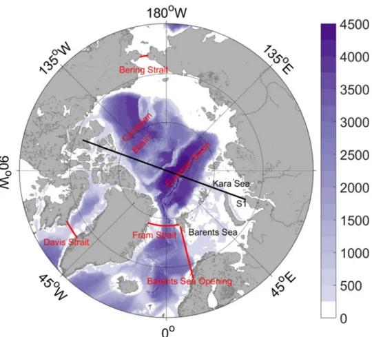
Different from the Arctic surface, deep, and bottom waters, the AW is characterized by its high temperature (defined by T > 0 °C). In this paper, the AW core tempera- ture (AWCT) and AW core depth (AWCD) during 1950 to 2005 from the CMIP5 models and their multimodel mean (MMM) are compared with those derived from the PHC3.0 dataset. Similar to previous studies (Polyakov et al. 2004; Li et al. 2012, 2014; Wang et al. 2018), the AWCT is defined as the maximum temperature below the halocline (150 m in this study) in the vertical profile, and the AWCD is defined as the depth of the AWCT. During our analysis, the Arctic deep basin (where ocean is deeper than 500 m) is divided into the Eurasian and Canadian basins separated by the Lomonosov Ridge, as shown in Fig. 1. In this study, correlation analy- sis is used to understand the relationship of AWCT bias to upstream conditions. The correlation coefficient used in this paper is Spearman’ rho, and the p value is computed using large-sample approximations. If the p value < 0.05, we con- sider the correlation to be significant.

3 Results

The water mass in the Arctic Ocean can be roughly divided into three layers: cold Polar Surface Water that extends from the sea surface to the depth of about 200 m, the relatively warm AW layer in the depth range of about 200–800 m, and deep/bottom waters that lie below the AW layer (Talley et al.

2011). The focus of this study is on the Arctic AW layer.

3.1 Temperature and salinity profiles

Basin mean vertical profiles of potential temperature and salinity in the Eurasian and Canadian basins are compared in Fig. 2. It can be seen that the CMIP5 models have relatively large intermodel spread in simulated temperature for the AW and deep/bottom waters (Fig. 2a, b). Most models have warm biases below the depth of 500 m. Below 1000 m, CMIP5 MMM temperature is about 1 °C warmer than the observa- tion and the bias is larger than in the CORE-II forced-model simulations (Ilicak et al. 2016). The maximum value in the vertical profile of the basin-mean temperature in the PHC3.0 dataset is about 1.2 °C and 0.4 °C in the Eurasian and Cana- dian basins, respectively (Fig. 2a, b). However, the CMIP5 has a large intermodel spread, with maximum values ranging from < −1 to > 5 °C (Fig. 2a, b).

The CMIP5 intermodel spread of simulated salinity is relatively small below the depth of 500 m, but large in the upper ocean (Fig. 2c, d). The basin-mean sea surface salin- ity ranges from < 30 to > 34 psu among the CMIP5 models.

Compared with the CORE-II salinity simulations (Ilicak et al. 2016), the CMIP5 models have larger salinity biases.

For the upper 200 m in the Eurasian Basin, the CMIP5 MMM salinity has a negative bias (− 1.0 psu) relative to the PHC3.0 dataset. The CORE-II model results also show a negative bias in this depth range, but with a smaller magni- tude (Ilicak et al. 2016). In the Canadian Basin, the CMIP5 MMM salinity has a positive bias in the upper 100 m and a negative bias between the depths of 100 and 500 m. Over- all, the signs of the salinity biases (negative or positive) in different depth ranges and basins are similar to standalone ocean-ice models shown by Ilicak et al. (2016), while the magnitudes of the biases are larger in the coupled climate models.

3.2 AWCD and AWCT

The observed AWCD in the Arctic Ocean is mainly in the depth range of 200–600 m (Ilicak et al. 2016). However, we find that the depth of the maximum temperature below the halocline in several CMIP5 models is much deeper than the observations (Fig. 3a, b). Models with the maximum

Table 1 Information regarding the CMIP5 models and PHC3.0 data- set used in this study

No. Name Grid number

x × y × z

1 ACCESS1.0 360 × 300 × 50

2 ACCESS1.3 360 × 300 × 50

3 BCC-CSM1.1(m) 360 × 232 × 40

4 BCC-CSM1.1 360 × 232 × 40

5 CCSM4 320 × 384 × 60

6 CESM1(BGC) 320 × 384 × 60

7 CESM1(CAM5.1, FV2) 320 × 384 × 60

8 CESM1(CAM5) 320 × 384 × 60

9 CESM1(FASTCHEM) 320 × 384 × 60

10 CESM1(WACCM) 320 × 384 × 60

11 CMCC-CESM 182 × 149 × 31

12 CMCC-CM 182 × 149 × 31

13 CMCC-CMS 182 × 149 × 31

14 CNRM-CM5 362 × 292 × 42

15 CanESM2 256 × 192 × 40

16 FIO-ESM 320 × 384 × 40

17 GFDL-CM2.1 360 × 200 × 50

18 GFDL-CM3 360 × 200 × 50

19 GFDL-ESM2G 360 × 210 × 50

20 GFDL-ESM2M 360 × 200 × 50

21 GISS-E2-H-CC 360 × 180 × 33

22 GISS-E2-H 360 × 180 × 33

23 GISS-E2-R-CC 288 × 180 × 32

24 GISS-E2-R 288 × 180 × 32

25 HadCM3 288 × 144 × 20

26 HadGEM2-AO 360 × 216 × 40

27 HadGEM2-CC 360 × 216 × 40

28 HadGEM2-ES 360 × 216 × 40

29 IPSL-CM5A-LR 182 × 149 × 31

30 IPSL-CM5A-MR 182 × 149 × 31

31 IPSL-CM5B-LR 182 × 149 × 31

32 MIROC-ESM 256 × 192 × 44

33 MIROC4h 1280 × 912 × 48

34 MIROC5 256 × 224 × 50

35 MPI-ESM-LR 256 × 220 × 40

36 MPI-ESM-MR 802 × 404 × 40

37 MPI-ESM-P 256 × 220 × 40

38 MRI-CGCM3 360 × 368 × 51

39 MRI-ESM1 360 × 368 × 51

40 NorESM1-M 320 × 384 × 53

41 NorESM1-ME 320 × 384 × 53

42 CMIP5 MMM 341 × 267 × 44

43 PHC3.0 (observation) 360 × 180 × 33

temperature located deeper than four times the observed depth in the Eurasian or Canadian basins are excluded from further analysis, because it is hard to properly clas- sify the AW layer within a reasonable depth range. Fol- lowing this criterion, nine CMIP5 models (ACCESS1.0, ACCESS1.3, BCC-CSM1.1, CanESM2, GISS-E2-H-CC, GISS-E2-H, MPI-ESM-LR, MPI-ESM-MR, and MRI- ESM1) are excluded (Fig. 3a, b). ACCESS1.0, ACCESS1.3, MPI-ESM-LR, MPI-ESM-MR, and MRI-ESM1 have much deeper AWCD in the Canadian basin, while BCC-CSM1.1, CanESM2, GISS-E2-H-CC, and GISS-E2-H have too deep AWCD in both the Eurasian and Canadian basins (Fig. S1).

The models with too large T/S biases, such as too low tem- perature (< −1 °C) or too high sea surface salinity (> 34 psu), can also be excluded by this criterion.

Even after excluding these models, the MMM AWCD remains deeper than in the PHC3.0 dataset (Fig. 3a, b).

The observed basin-mean AWCD in the PHC3.0 dataset is about 310 m and 460 m in the Eurasian and Canadian basins, respectively, whereas the CMIP5 MMM AWCD is 680 m and 830 m, respectively. Only three models (HadGEM2-AO, HadGEM2-CC, and HadGEM2-ES) in the Eurasian Basin and five models (GISS-E2-R-CC, GISS-E2-R, HadGEM2- AO, HadGEM2-CC, and HadGEM2-ES) in the Canadian Basin produced slightly shallower AWCD than the PHC3.0

dataset. Therefore, the problem of the AW layer being too deep, reported for AOMIP and CORE-II models (Holloway et al. 2007; Ilicak et al. 2016), also exists in the CMIP5 coupled models.

The AWCT from the CMIP5 models and PHC3.0 dataset in the two basins is shown in Fig. 3c, d, respectively. The MMM AWCT shows a warm bias compared to the obser- vations. The basin-mean AWCT from the PHC3.0 dataset is about 1.1 °C and 0.5 °C in the Eurasian and Canadian basins, respectively. The CMIP5 MMM warm bias is about 0.2 °C and 0.5 °C in these two basins, respectively.

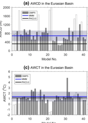
The CMIP5 models have very large intermodel spread in the simulated AWCD and AWCT (Fig. 3). The AWCD has a standard deviation of about 240 m and 300 m in the Eurasian and Canadian basins, respectively. The minimum and maxi- mum AWCDs in the Eurasian Basin are 250 m (HadGEM2- CC) and 1220 m (MRI-CGCM3), respectively (after exclud- ing the nine models mentioned above). In the Canadian Basin, the basin mean AWCD is in the range 320–1370 m.

For the AWCT, the standard deviation is about 0.9 °C and 1.0 °C in the Eurasian and Canadian basins, respectively.

The IPSL-CM5B-LR model has the warmest AWCTs with basin-mean values of 4.8 °C and 4.2 °C in the Eurasian and Canadian basins, respectively. The GFDL-ESM2G and HadGEM2-ES models have the coldest AWCTs with values

Fig. 1 Arctic Ocean bottom topography (unit: m). Red lines indicate the main Arctic gate- ways and the black line crossing the North Pole indicates the location of section S1 used in Fig. 5 and the supplementary Figs. S1 and S3

of about 0.1 °C and − 0.2 °C in the Eurasian and Canadian basins, respectively.

The spatial patterns of AWCT and AWCD are related to the AW circulation pathways in the Arctic basins. In the

Arctic Ocean, the AW follows a path that is mainly cyclonic along the continental slope and mid-ocean ridges, i.e., a topographically steered boundary current (Rudels et al.

1994). The AW from the Fram Strait flows eastward along 0

500 1000 1500 2000 2500 3000 3500

Depth (m)

-2 -1

Temperature (^oC)

(a)

PHC3.0 MMM

0 500 1000 1500 2000 2500 3000 3500

Depth (m)

-2 -1

0 1 2 3 4 5 0 1 2 3 4 5

Temperature (^oC)

(b)

PHC3.0 MMM

0 200 400 600 800 1000 1200 1400 1600

Depth (m)

30 31 32 33 34 35 36

Salinity (psu)

(c)

PHC3.0 MMM

0 200 400 600 800 1000 1200 1400 1600

Depth (m)

30 31 32 33 34 35 36

Salinity (psu)

(d)

PHC3.0 MMM

Fig. 2 Profiles of basin mean potential temperature (a, b, unit: °C) and salinity (c, d, unit: psu) in the Eurasian and Canadian basins. Thin lines represent the 41 CMIP5 models, and the thick black and blue lines represent the PHC3.0 dataset and the CMIP5 MMM, respectively

the Eurasian slope, converges with the AW from the Barents Sea Opening (BSO) at the St. Anna Trough (Schauer et al.

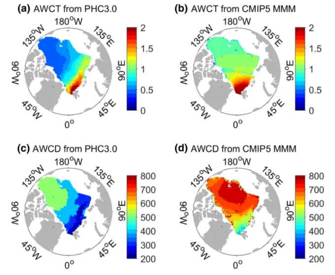
2002a; Karcher and Oberhuber 2002), and then flows east- ward along the continental slope. After passing the Laptev Sea slope, the AW circulation divides into two branches: one along the Lomonosov Ridge toward the Fram Strait and the other along the continental slope toward the Canadian Basin (Woodgate et al. 2001). Along the pathways, the AWCT decreases gradually. It is around 3 °C near the Fram Strait, and decreases gradually to about 0.8 °C near the Lomonosov Ridge and to about 0.4 °C in the Canada Basin (Fig. 4a). The AWCD deepens from the depth of 200 m in the Fram Strait to about 350 m near the Lomonosov Ridge, and to about 500 m in the Canada Basin (Fig. 4c). These changes are due to mixing from both above and below and with shelf waters (Talley et al. 2011).

Figure 4b shows that the CMIP5 MMM AWCT is high near the Fram Strait and low in the Canadian Basin, simi- lar to that in the observations. However, the CMIP5 MMM

AWCT is higher than the observed in most regions of the Arctic Ocean, and the gradient from warm to cold regions is different from the observed. For the simulated AWCD, the CMIP5 MMM is shallow in the Fram Strait and deep in the Canada Basin. However, it is much deeper than in the PHC3.0 dataset for almost the entire Arctic Ocean (Fig. 4d).

The spatial patterns of both the AWCT and the AWCD have large biases in the Canadian Basin. In the PHC3.0 dataset, low AWCTs and deep AWCDs are found mainly in the southeastern Canadian Basin. In the CMIP5 MMM results, a tongue of relatively warm water extends directly from the Laptev Sea slope towards north of Greenland through the North Pole, implying that the simulated AW pathways are not well along the bottom topography (Fig. 4b). The MMM AWCD is deepest in the region close to the East Siberian continental slope (Fig. 4d), different from the observation.

Inspecting individual models reveals that most of them cannot adequately reproduce the observed topography-fol- lowing feature of the AW circulation (Fig. S2). This might

Fig. 3 a, b Atlantic Water core depth (AWCD; unit: m) and c, d Atlantic Water core temperature (AWCT; unit: °C) derived from the CMIP5 models and PHC3.0 dataset for the Eurasian and Canadian basins. Bars are for the individual CMIP5 models. White bars repre- sent models unable to represent the Atlantic Water (AW) layer in one or two Arctic basins; see text for details. Blue and black lines repre-

sent the CMIP5 MMM and the PHC3.0 dataset, respectively. Shaded area represents MMM ± one standard deviation. The models unable to represent the AW layer in the Arctic basins (shown by white bars) are excluded in the MMM and other analysis, the same in other figures in the paper. The x axis shows the model number and the corresponding model name can be found in Table 1

be attributed to the unrealistic Arctic Circumpolar Boundary Current in the coarse-resolution models. The AW pathways are along topographically steered boundary currents, which follow continental slopes or the mid-ocean ridges. However, the nominal resolution of about 1° in most CMIP5 models is too coarse and the spurious dissipation leads to a weak and wide Arctic Circumpolar Boundary Current (Fig. S2). It is suggested that this problem could be alleviated by including Neptune parameterization of eddy–topography interaction (Holloway 1986, 1987; Polyakov 2001; Golubeva and Pla- tov 2007; Li et al. 2013) or by improving model resolution (Li et al. 2013; Wang et al. 2018). However, the MIROC4h model (Sakamoto et al. 2012), which has the highest reso- lution among the CMIP5 models (0.28125° × 0.1875°), is also subject to this common problem (Fig. S2). This may indicate that higher (eddy-resolving) horizontal resolution is needed in the AW simulations, while we cannot exclude some other unknown reasons. The isopycnal-coordinate ocean model in NorESM1-M and NorESM1-ME produces better results, which is very possibly due to the fact that

advection operators in isopycnal coordinates do not allow for spurious diapycnal mixing (Griffies 2004).

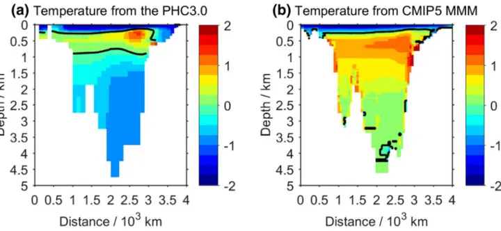
3.3 Temperature vertical section

To assess the AW layer thickness, a vertical section of poten- tial temperature between 70°E and 110°W along section S1 (indicated in Fig. 1) from the PHC3.0 dataset and the CMIP MMM is shown in Fig. 5a, b, respectively. This section can easily capture the spatial gradient of temperature in the Arc- tic Ocean. If the AW layer is defined as the layer with poten- tial temperature > 0 °C (Holloway et al. 2007), the AW layer thickness in the PHC3.0 dataset is about 700 m (Fig. 5a).

The observed upper boundary of the AW layer along section S1 is at the depth of about 200 m (slightly shallower in the Eurasian Basin and deeper in the Canadian Basin), and the lower boundary is at the depth of about 800 m.

It can be seen that the CMIP5 MMM tends to produce a too thick AW layer in comparison with the PHC3.0 dataset (Fig. 5b). The depth of the upper boundary of the

Fig. 4 a, b AWCT (unit: °C) and c, d AWCD (unit: m) from PHC3.0 and CMIP5 MMM

AW layer is reasonable, while the lower boundary of the AW layer is too deep and almost reaches the bottom of the Arctic Ocean. This is most possibly the consequence of too much spurious diapycnal mixing associated with coarse resolution models. Spurious mixing is expected to decrease with increasing resolution. By increasing hor- izontal resolution to 4.5 km in the Arctic Ocean while keeping vertical resolution the same, Wang et al. (2018) obtained realistic AW layer thickness. The vertical sec- tion of potential temperature along section S1 for each CMIP5 model is shown in Figure S3. Most CMIP5 mod- els simulated a too thick AW layer. Only a few models (GISS-E2-R-CC, GISS-E2-R, HadGEM2-AO, HadGEM2- CC, NorESM1-M, and NorESM1-ME) produced relatively reasonable AW layer thickness. These models also better simulated AWCD (Fig. 3). The isopycnal-coordinate ocean model in NorESM1-M and NorESM1-ME produced better results in this respect too by eliminating spurious diapy- cnal mixing.

The problem of too deep and too thick AW layer in the Arctic basins could also be partly attributed to the upstream condition, the AW properties in the Fram Strait.

Figure S4 shows that the AW in the Fram Strait in most CMIP5 models has already the characteristics of being too deep and too thick in comparison with the PHC3.0 dataset. The characteristics of the AW in the Fram Strait can propagate into the Arctic basins, explaining part of the biases inside the Arctic Ocean. This suggests that spurious mixing associated with coarse resolution both outside and inside the Arctic Ocean causes the obtained biases in the Arctic Ocean.

3.4 Relationship of AW temperature bias to upstream conditions

Analysis of forced ocean-ice models showed that the per- formance of the simulated AW inflow through the Arctic gates could explain some of the biases in the Arctic AW temperature (Ilicak et al. 2016). In the following we will also investigate possible causes of the biases in the simulated AWCT in the CMIP5 models.

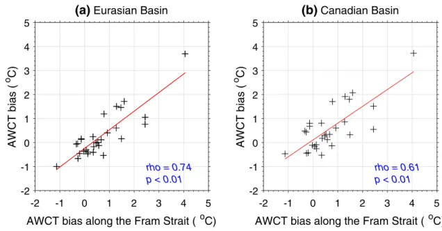
AW enters the Arctic Ocean via warmer (Fram Strait) and cooler (Barents Sea) branches. Figure 6 shows the relation- ship of the AWCT bias in the Arctic basins to the AWCT bias in the Fram Strait in the CMIP5 models. Three mod- els (HadGEM2-AO, HadGEM2-CC, and HadGEM2-ES), which cannot resolve the topography in the Fram Strait due to coarse resolution, are excluded in the plots (their model topography is about 1000 m instead of about 4000 m, see Fig. S4). Significant correlation is found between the AWCT bias in the Arctic basins and the AWCT bias in the Fram Strait in the CMIP5 models (Fig. 6), with the Spearman’s correlation coefficient for the Eurasian Basin (0.74) being slightly larger than for the Canadian Basin (0.61). Models with large AWCT bias are those with a large temperature bias in the Fram Strait.

Another branch of AW flows into the Barents Sea through the BSO, where the water is exposed to the air above and vertically mixed and cooled very efficiently in winter time (Smedsrud et al. 2013). This cooled branch flows into the Arctic basins via the St. Anna Trough in the northern Kara Sea, where part of the AW converges with the warmer branch from the Fram Strait (Schauer et al. 2002a; Karcher

Fig. 5 Vertical section of water temperature (unit: °C) between 70°E and 110°W along section S1 (Fig. 1) from a the PHC3.0 dataset and b the CMIP5 MMM. Black line is the 0 °C isotherm

and Oberhuber 2002). Figure 7 shows that there is significant correlation between the AWCT biases in the Arctic basins and the temperature biases in the whole Kara Sea in the CMIP5 climate models. The Spearman’s correlation coef- ficient for the Eurasian Basin (0.71) is also slightly larger than for the Canadian Basin (0.67). The high correlation reveals that the Arctic Ocean AWCT biases in the CMIP5 models are also related to temperature biases in the Barents Sea AW branch.

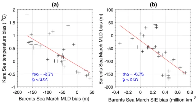
Cooling of the AW passing through the Barents Sea plays a crucial role in the ventilation of the Arctic Ocean (Schauer et al. 2002b). The winter cooling of the AW in the Barents Sea generates relatively deep upper mixed layer and cold dense water, which passes the Kara Sea before penetrating into the Arctic deep basin. Significant correlation between Kara Sea temperature biases and the Barents Sea March mixed-layer depth (MLD) biases (Fig. 8a), and between the Barents Sea March MLD biases and the Barents Sea March

-2 -1 0 1 2 3 4 5

AWCT bias along the Fram Strait ( ^oC) -2

-1 0 1 2 3 4 5

AWCT bias (o C)

(a)

rho = 0.74 p < 0.01

-2 -1 0 1 2 3 4 5

AWCT bias along the Fram Strait ( ^oC) -2

-1 0 1 2 3 4 5

AWCT bias (o C)

(b)

rho = 0.61 p < 0.01

Fig. 6 Relationship of Atlantic Water core temperature (AWCT) biases in the a Eurasian and b Canadian basins to AWCT biases in the Fram Strait. The models numbered 26–28 are not included. The latter models have too shallow ocean depth in the Fram Strait (see Fig. S4)

-1 -0.5 0 0.5 1 1.5 2

Kara Sea temperature bias (^oC) -2

-1 0 1 2 3 4

AWCT bias (o C)

(a)

rho = 0.71 p < 0.01

-1 -0.5 0 0.5 1 1.5 2

Kara Sea temperature bias (^oC) -2

-1 0 1 2 3 4

AWCT bias (o C)

(b)

rho = 0.67 p < 0.01

Fig. 7 Relationship of AWCT biases in a the Eurasian Basin and b the Canadian Basin to the Kara Sea temperature biases in the CMIP5 models

sea ice extent (SIE, Fig. 8b) are found in the CMIP5 models.

Models with shallow wintertime MLD in the Barents Sea usually have warm biases in the Kara Sea. Too shallow win- tertime MLD means that the AW in the Barents Sea is not cooled efficiently. Figure 8b further suggests that the mod- els with too shallow wintertime MLD usually have greater SIE in winter. Increased coverage of sea ice will limit the air–sea heat exchange in these models and cause inefficient cooling of the AW in the Barents Sea. Thus, excessive heat is transported into the Kara Sea and then into the Arctic basins. Onarheim et al. (2015), Wang et al. (2016) and Li et al. (2017) indicate that the Barents Sea SIE is correlated with heat inflow through the BSO. So models with greater heat inflow via the BSO usually have less sea ice coverage, release more heat into the air over the Barents Sea, and then have cold biases in the Arctic Ocean. Therefore, Barents Sea cooling is also a crucial factor impacting the AWCT in climate models, similar to the finding based on forced ocean- ice models in Ilicak et al. (2016).

3.5 Variability and trend

Long-term observations during the twentieth century revealed that the AW layer of the Arctic Ocean is fea- tured with low-frequency oscillation on the timescale of 50–80 years (Polyakov et al. 2004). For the past several dec- ades, the AW layer in the Arctic Ocean has experienced a warming trend (Polyakov et al. 2004, 2012). Based on analy- sis of an extensive array of observations in the Arctic deep basin obtained during 1950–2011, Polyakov et al. (2012)

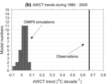
concluded that significant warming has started since the late 1970s (Fig. 9).

The CMIP5 models did not reproduce the observed warm- ing trend of the Arctic AW layer (Fig. 9). The observed lin- ear trend of AWCT is 0.66 °C decade⁻¹ during 1980–2005, whereas the CMIP5-simulated AWCT is very stable without significant trends. Figure 9b shows that 8 CMIP5 models produced slight cooling trends and 24 CMIP5 models pro- duced very weak warming trends during 1980–2005. The HadGEM2-AO model produced the largest warming trend (0.074 °C decade⁻¹). This might be related to HadGEM2- AO having a more realistic AW layer thickness (Figure S3).

But its trend is still much smaller than the observed. Fig- ure 9a also shows that interannual variability in the CMIP5 models is very small and much weaker than the observed.

4 Discussions and conclusions

In this study we assessed the AW layer of the Arctic Ocean in 41 CMIP5 coupled climate models. Nine of the CMIP5 models did not reproduce a well-defined AW layer. Although the MMM results derived from the remaining 32 CMIP5 models can reproduce the main spatial patterns of the AWCT and the AWCD, the simulated AW layer is too deep and thick. This is also a common problem in state-of-the-art standalone ocean-ice models (Li et al. 2014; Ilicak et al.

2016). Spurious numerical dissipation was considered to be one of the key reasons for the deepening and thickening of the AW layer (Holloway et al. 2007).

-200 -150 -100 -50 0 50 Barents Sea March MLD bias (m) -1

-0.5 0 0.5 1 1.5 2

Kara Sea temperature bias (o C)

(a)

rho = -0.71 p < 0.01

-0.4 -0.2 0 0.2 0.4 0.6 0.8 Barents Sea March SIE bias (million km ²) -200

-150 -100 -50 0 50 100

Barents Sea March MLD bias (m)

(b)

rho = -0.75 p < 0.01

Fig. 8 Relationships among Kara Sea temperature biases, Barents Sea March mixed-layer depth (MLD) biases, and Barents Sea March sea ice extent (SIE) biases in the CMIP5 models

The CMIP5 models show large intermodel spreads in the simulated Arctic hydrography, AWCT and AWCD. Our analysis indicates that the AWCT biases in the Arctic basins are related to the AW temperature bias in the Fram Strait and the ocean temperature in the Barents and Kara seas.

We suggest that the performance in the simulation of sea ice coverage and surface cooling in the Barents Sea is one of the key factors that can influence the fidelity of the AW layer in the models.

The interannual variability of the AWCT in the CMIP5 models is much weaker than the observed. No CMIP5 model can reproduce the observed significant warming trend in the AW layer of the Arctic Ocean in the past decades. The recently observed “Atlantification” of the eastern Eurasian Basin implies increasing impacts of the AW layer on the sea ice state (Polyakov et al. 2017). Failing to simulate the warming trend of the AW layer (or delay in capturing the warming trend) can prevent climate models from being applied in studies on the impacts of “Atlantification” in the warming climate.

Many factors in models might affect the simulation of the AW layer in the Arctic Basin, e.g., model resolution, vertical mixing, eddy and eddy–topography interaction parameterizations, advection schemes, and representation of import of thermal and freshwater anomalies through Arctic gates (Morales Maqueda and Holloway 2006;

Zhang and Steele 2007; Holloway et al. 2007; Li et al.

2011, 2013; Wang et al. 2018). Previous studies have shown that the common problems in simulating the AW layer in standalone ocean-ice models could be alleviated by incorporating high-order advection schemes (Morales

Maqueda and Holloway 2006; Holloway et al. 2007), including eddy–topography interaction parameterization (e.g., Golubeva and Platov 2007; Holloway and Wang 2009; Li et al. 2013), tuning background vertical mix- ing coefficients (Zhang and Steele 2007), or increasing model horizontal resolution (e.g., Li et al. 2013; Wang et al. 2018). Our results show that the temperature and salinity biases in coupled climate models are larger than in standalone ice–ocean models. Therefore, to improve the representation of the AW layer in climate models, such measures should also be tested and studied by different model development groups.

In the coming CMIP6 phase, many modeling groups will use improved model versions and better resolutions.

We expect to see improvement in the model representation of the Arctic Ocean in the new simulations, which need to be accessed when results become available.

Acknowledgements The output of the CMIP5 coupled models were downloaded from http://pcmdi 9.llnl.gov/esgf-web-fe/. The PHC3.0 dataset was downloaded from http://psc.apl.washi ngton .edu/nonwp _proje cts/PHC/Clima tolog y.html. The authors would like to thank the above data providers. Qi Shu was supported by the National Key Research and Development Program of China (Grant No. 2016YFC1401407), and the Basic Scientific Fund for National Public Research Institute of China (ShuXingbei Young Talent Pro- gram 2019S06). Jie Su was supported by the Global Change Research Program of China (Grant No. 2015CB953900) and National Natural Science Foundation of China (Grant No. 41330960). Fangli Qiao was supported by NSFC-Shandong Joint Fund for Marine Science Research Centers (Grant No. U1406404). We thank Igor V. Polyakov for provid- ing long-term observation dataset. We wish to express our gratitude to the two reviewers and the editor for their helpful comments.

Fig. 9 a Time series of Arctic mean AWCT anomalies over 1950–

2005 and b the AWCT trends during 1980–2005 in the CMIP5 simulations and observations. Observations are from Polyakov et al.

(2012). In a thin lines represent individual CMIP5 simulations and

the thick black line represents the observations. Anomalies are refer- enced to the 1950 value. Bars in b represent the number of CMIP5 models that have the AWCT trend indicated by the x axis. Thick black line in b represents the observed AWCT trend

Open Access This article is distributed under the terms of the Crea- tive Commons Attribution 4.0 International License (http://creat iveco mmons .org/licen ses/by/4.0/), which permits unrestricted use, distribu- tion, and reproduction in any medium, provided you give appropriate credit to the original author(s) and the source, provide a link to the Creative Commons license, and indicate if changes were made.

References

Aagaard K, Swift JH, Carmack EC (1985) Thermohaline circula- tion in the Arctic Mediterranean Seas. J Geophys Res Oceans 90(C3):4833–4846

Beszczynska-Moller A, Fahrbach E, Schauer U et al (2012) Variability in Atlantic water temperature and transport at the entrance to the Arctic Ocean, 1997–2010. ICES J Mar Sci 69(5):852–863 Dickson B, Meincke J, Rhines P (2008) Arctic–subarctic ocean fluxes:

defining the role of the Northern Seas in climate. In: Arctic–Sub- arctic Ocean fluxes. Springer Netherlands, Dordrecht

Golubeva EN, Platov GA (2007) On improving the simulation of Atlan- tic water circulation in the Arctic Ocean. J Geophys Res Oceans 112(C4):1–16

Griffies SM (2004) Fundamentals of ocean climate models. Princeton University Press, Princeton

Griffies SM, Biastoch A, Böning C et al (2009) Coordinated ocean-ice reference experiments (COREs). Ocean Model 26(1):1–46 Hattermann T, Isachsen PE, von Appen WJ et al (2016) Eddy-driven

recirculation of Atlantic water in Fram Strait. Geophys Res Lett 43(7):3406–3414

Holloway G (1986) A shelf wave/topographic pump drives mean coastal circulation. Ocean Model 68:12–15

Holloway G (1987) Systematic forcing of large-scale geophysical flows by eddy-topography interaction. J Fluid Mech 184:463–476 Holloway G, Wang Z (2009) Representing eddy stress in an Arctic

Ocean model. J Geophys Res Oceans 114:C06020. https ://doi.

org/10.1029/2008j c0051 69

Holloway G, Dupont F, Golubeva E et al (2007) Water properties and circulation in Arctic Ocean models. J Geophys Res Oceans 112(C4):225–237

Ilicak M, Drange H, Wang Q et al (2016) An assessment of the Arctic Ocean in a suite of interannual CORE-II simulations. Part III:

hydrography and fluxes. Ocean Model 100:141–161

Ivanov V, Smirnov A, Alexeev V et al (2018) Contribution of con- vection-induced heat flux to winter ice decay in the Western Nansen Basin. J Geophys Res Oceans 123:6581–6597. https ://

doi.org/10.1029/2018J C0139 95

Karcher MJ, Oberhuber JM (2002) Pathways and modification of the upper and intermediate waters of the Arctic Ocean. J Geophys Res Oceans 107:3049. https ://doi.org/10.1029/2000J C0005 30 Karcher M, Gerdes R, Kauker F et al (2003) Arctic warming: Evolu-

tion and spreading of the 1990s warm event in the Nordic seas and the Arctic Ocean. J Geophys Res 108(C2):3034. https ://doi.

org/10.1029/2001J C0012 65

Karcher M, Beszczynskamoller A, Kauker F et al (2011) Arctic Ocean warming and its consequences for the Denmark Strait overflow. J Geophys Res 116:C02037. https ://doi.org/10.1029/2010J C0062 65 Li X, Su J, Zhang Y et al (2011) Discussion on the simulation of Arctic

Intermediate Water under the NEMO modeling framework. In:

The proceedings of the twenty first (2011) international offshore and polar engineering conference, vol 1, pp 953–957

Li S, Zhao J, Su J et al (2012) Warming and depth convergence of the Arctic Intermediate Water in the Canada Basin during 1985–2006.

Acta Oceanol Sin 31(4):46–54

Li X, Su J, Wang Z et al (2013) Modeling Arctic intermediate water:

the effects of Neptune parameterization and horizontal resolution.

Adv Polar Sci 24(2):98–105

Li X, Su J, Zhao J (2014) An evaluation of the simulations of the Arctic intermediate water in climate models and reanalyses. Acta Oceanol Sin 33(12):1–14

Li D, Zhang R, Knutson TR (2017) On the discrepancy between observed and CMIP5 multi-model simulated Barents Sea winter sea ice decline. Nat Commun 8:14991

Marnela M, Rudels B, Houssais MN et al (2013) Recirculation in the Fram Strait and transports of water in and north of the Fram Strait derived from CTD data. Ocean Sci 9:499–519

Maslowski W, Marble D, Walczowski W et al (2004) On climato- logical mass, heat, and salt transports through the Barents Sea and Fram Strait from a pan-Arctic coupled ice-ocean model simulation. J Geophys Res Oceans 109:C03032. https ://doi.

org/10.1029/2001J C0010 39

Morales Maqueda MA, Holloway G (2006) Second-order moment advection scheme applied to Arctic Ocean simulation. Ocean Model 14(3):197–221

Onarheim IH, Eldevik T, Årthun M et al (2015) Skillful prediction of Barents Sea ice cover. Geophys Res Lett 42(13):5364–5371 Orvik KA, Niiler P (2002) Major pathways of Atlantic water in the

northern North Atlantic and Nordic Seas toward Arctic. Geo- phys Res Lett 29(19):2-1–2-4

Polyakov IV (2001) An eddy parameterization based on maximum entropy production with application to modeling of the Arctic Ocean circulation. J Phys Oceanogr 31(8):2255–2270 Polyakov IV, Alekseev GV, Timokhov LA et al (2004) Variability

of the intermediate Atlantic water of the Arctic Ocean over the last 100 years. J Climate 17(23):4485–4497

Polyakov IV, Timokhov L, Alexeev VA et al (2010) Arctic Ocean warming contributes to reduced polar ice cap. J Phys Oceanogr 40(12):2743–2756

Polyakov IV, Pnyushkov AV, Timokhov LA (2012) Warming of the intermediate Atlantic water of the Arctic Ocean in the 2000s. J Climate 25(25):8362–8370

Polyakov IV, Bhatt US, Walsh J et al (2013) Recent oceanic changes in the Arctic in the context of long-term observations. Ecol Appl 23(8):1745–1764

Polyakov IV, Pnyushkov AV, Alkire MB et al (2017) Greater role for Atlantic inflows on sea-ice loss in the Eurasian Basin of the Arctic Ocean. Science 356(6335):285–291

Proshutinsky A, Kowalik Z (2007) Preface to special section on Arctic Ocean Model Intercomparison Project (AOMIP) studies and results. J Geophys Res 112:C04S01. https ://doi.

org/10.1029/2006J C0040 17

Proshutinsky A, Aksenov Y, Kinney JC et  al (2011) Recent advances in Arctic Ocean studies employing models from the Arctic Ocean model intercomparison project. Oceanography 24(3):102–113

Rudels B, Friedrich HJ (2000) The transformations of Atlantic water in the Arctic Ocean and their significance for the freshwater budget. In: Lewis EL, Jones EP, Lemke P, Prowse TD, Wadhams P (eds) The freshwater budget of the Arctic Ocean. Springer, Dordrecht, pp 503–532

Rudels B, Jones EP, Anderson LG et al (1994) On the intermediate depth waters of the Arctic Ocean. In: The Polar Oceans and their role in shaping the global environment. American Geo- physical Union, p 470

Sakamoto TT, Komuro Y, Nishimura T et al (2012) MIROC4h—a new high-resolution atmosphere-ocean coupled general circula- tion model. J Meteorol Soc Jpn 90(3):325–359

Schauer U, Loeng H, Rudels B et al (2002a) Atlantic water flow through the Barents and Kara Seas. Deep Sea Res Part I 49(12):2281–2298

Schauer U, Rudels B, Jones EP et al (2002b) Confluence and redistri- bution of Atlantic water in the Nansen, Amundsen and Makarov basins. Ann Geophys 20(2):257–273

Schauer U, Beszczynska-Möller A, Walczowski W et al (2008) Varia- tion of measured heat flow through the Fram Strait between 1997 and 2006. In: Dickson RR, Meincke J, Rhines P (eds) Arctic- Subarctic ocean fluxes: defining the role of the Northern Seas in climate. Springer, Dordrecht, pp 65–85

Smedsrud LH, Esau I, Ingvaldsen RB et al (2013) The role of the Bar- ents Sea in the arctic climate system. Rev Geophys 51(3):415–449 Steele M, Morley R, Ermold W et al (2001) PHC: a global ocean

hydrography with a high-quality Arctic Ocean. J Climate 14(9):2079–2087

Talley LD, Pickard GL, Emery WJ et al (2011) Descriptive physical oceanography: an introduction, 6th edn. Academic Press, London Wang Q, Ilicak M, Gerdes R et al (2016) An assessment of the Arctic

Ocean in a suite of interannual CORE-II simulations. Part I: sea ice and solid freshwater. Ocean Model 99:110–132

Wang Q, Wekerle C, Danilov S et al (2018) A 4.5 km resolution Arctic Ocean simulation with the global multi-resolution model FESOM 1.4. Geosci Model Dev 11:1229–1255

Wekerle C, Wang Q, Von Appen W et al (2017) Eddy-resolving simula- tion of the atlantic water circulation in the Fram strait with focus on the seasonal cycle. J Geophys Res 122(11):8385–8405 Woodgate RA, Aagaard K, Muench RD et al (2001) The Arctic

ocean boundary current along the Eurasian slope and the adja- cent lomonosov ridge: water mass properties, transports and transformations from moored instruments. Deep Sea Res Part I 48(8):1757–1792

Zhang J, Steele M (2007) Effect of vertical mixing on the Atlantic Water layer circulation in the Arctic Ocean. J Geophys Res 112:C04S04. https ://doi.org/10.1029/2006j c0037 32

Publisher’s Note Springer Nature remains neutral with regard to jurisdictional claims in published maps and institutional affiliations.