On the restrictiveness of equality constraints in multivariate curve resolution Mathias Sawall

(1)

On the restrictiveness of equality constraints in multivariate curve resolution

Mathias Sawallâ, Somaye Vali Zade^b, Christoph Kubis^c, Henning Schröderâ,c, Denise Meinhardtâ,c, Alexander Brächer^d, Robert Franke^d,e, Armin Börner^c, Hamid Abdollahi^b, Klaus Neymeyrâ,c

aUniversit¨at Rostock, Institut f¨ur Mathematik, Ulmenstraße 69, 18057 Rostock, Germany

bFaculty of Chemistry, Institute for Advanced Studies in Basic Sciences, 45195-1159 Zanjan, Iran

cLeibniz-Institut f¨ur Katalyse, Albert-Einstein-Straße 29a, 18059 Rostock

dEvonik Performance Materials GmbH, Paul-Baumann Straße 1, 45772 Marl, Germany

eLehrstuhl f¨ur Theoretische Chemie, Ruhr-Universit¨at Bochum, 44780 Bochum, Germany

Abstract

Multivariate curve resolution methods suffer from the non-uniqueness of the solutions of the nonnegative matrix factorization problem. The solution ambiguity can be considerably reduced by equality constraints in the form of known spectra or concentration profiles. Two measures are suggested that indicate the impact of the equality constraints.

The representation of these measures in the area of feasible solutions show strong variations in the restrictiveness of equality constraints. The measures are tested for a three-component model problem and experimental data sets from the hydroformylation process and a catalyst cluster formation.

Key words: multivariate curve resolution, rotational ambiguity, area of feasible solutions, Borgen plot, equality constraint.

1. Introduction

Multivariate curve resolution (MCR) methods aim at the extraction of pure component information from spectral mixtures [13, 3, 15, 14, 19]. Typically, the spectral data is given on a time×frequency-grid in form of an absorption matrixD∈R^k×n. Therein,kis the number of spectra andnis the number of frequency channels. The Lambert-Beer law predicts thatDcan, at least approximately, be represented as the product of a concentration matrixC ∈R^k×sand a matrix of pure component spectraS ∈R^n×s, see [15, 11, 14]. Thereinsis the number of chemical components. The resulting pure component factorsCandS are nonnegative matrices. Typically, many nonnegative matrix factorizations D≈CS^Texist. The chemically correct factors are among all these nonnegative matrix factorizations. These facts are well known under the keyword of therotational ambiguityof the factorization [30, 1]. The so-called Area of Feasible Solutions (AFS) is a low-dimensional representation of this ambiguity [6, 25, 5, 21]. Two AFS sets exist for a data matrixD. The first one represents the possible concentration profiles and is denoted byM_C. The second one contains representations of the possible pure component spectra and is denoted byM_S.

The rotational ambiguity can be considerably reduced by known spectra or concentration profiles. For instance, a pure component spectrum of a reactant or of a reaction product might be known or a concentration profile of a certain component can sometimes be measured. Such additional knowledge on the reaction system can be fed into the factorization process in form of so-called equality constraints. The effect of equality constraints on the reduction of the rotational ambiguity can be very different. The relative position of the known component in the AFS related to the certain polygons, namely the inner polygon and the outer polygon, explains the behavior. The aim of this paper is to suggest two measures of ambiguity reduction. To each point of the AFS we assign a characteristic number that estimates the size of the AFS after addition of the equality constraints. As the size of the AFS correlates to some extent to the rotational ambiguity we consider these measures as ambiguity estimators.

These characteristic numbers can also be considered asrestrictiveness measures. A relatively large reduced AFS shows that the equality constraint cannot significantly reduce the rotational ambiguity. The profile that is locked by the equality constraint is compatible to many other solutions. In contrast to this a small reduced AFS means that the choice of the equality constraint is very restrictive for the factorization problem. We summarize these notions as follows:

An equality constraint strongly reduces the AFS if it has a highrestrictiveness. Similarly, a weak AFS reduction corresponds to a low restrictiveness. Then the fixed profile is compatible to many other spectral or concentration profiles.

(2)

2. Conceptual basis

2.1. The area of feasible solutions

The pure component factorsCandS can be constructed by means of a truncated singular value decomposition (SVD)D=UΣV^TofD, see [13, 14, 16]. The matricesUandVare truncated to their firstscolumns andΣis truncated to its leadings-by-ssubmatrix. IfDis of ranks, then the truncated SVD equalsD. Otherwise, the truncated SVD is the best approximation toDin terms of the spectral norm or the Frobenius norm among all rank-smatrices. Then the truncated factorsUandVare appropriate bases for the construction of the factorization. The factorsCandS of any (approximate) factorizationCS^Tcan be shown to be of the formC=UΣT⁻¹andS^T =T V^Tfor proper regulars-by-s matricesT. Thus all regular matricesT ∈R^s×sare to be determined so thatCandS are componentwise nonnegative matrices. However, the handling of sets ofs-by-smatrices is complicated and it is not clear how to present the results graphically even for smalls. Instead one can consider only the set of all columns ofCand also the set of all columns ofS that can appear in all nonnegative factorizationsD=CS^T respectively nonnegative approximate factorizations D≈CS^T. The vectors of these sets are still high-dimensional, namely either of the dimensionkor of the dimension n. The remedy is a representation of these vectors with respect to the bases of left and right singular vectors. Together with a certain scaling, this results in the Area of Feasible Solutions (AFS) representation of the feasible factors. This allows us to assume the possible matricesT to be of the 2-by-2 block form

T = 1 x^T

1 W

!

. (1)

Therein1is the all-ones column vector1=(1, . . . ,1)^T ∈R^s−1. The spectral AFS is defined to be

MS ={x∈R^s−1: existsW∈R^s−1×s−1with rank(T)=sandC=UΣT⁻¹≥0,S^T =T V^T ≥0}.

The concentration factor AFSMCfor feasibley∈R^s−1can be defined in an analogous way [22]. See [6, 25, 5, 21, 22]

for more details on the AFS-approach. Further, the so-called outer polygonsFS,FCand the inner polygonsIS,IC

are very important for the understanding and the construction of the AFS; see the references above for details on these polygons.

Several methods are available for the computation of the AFS. For two-component systems (s=2) the boundaries of the AFS, so-called Lawton-Sylvestre plots, are accessible analytically [13, 21] or alternatively by using numerical grid-search optimization [30, 1]. For three-component systems (s=3) geometric constructions [3, 18, 9] are available as well as numerical approximation methods [6, 25, 27, 28]. For the computations in this paper we use the newer dual Borgen plots method [22, 26].

2.2. Restrictiveness estimation by measuring the reduced rotational ambiguity

Letxbe an arbitrary point in the spectral AFSM_S. Thenxrepresents a certain spectrum. Next we assume this spectrum to be known. This means that we can fixxin the form of an equality constraint. The following step is the computation of the restricted AFS for the remainings−1 chemical components. In other words, we determine the possible rows ofWin (1) with (1,x^T) forming its first row so thatT is a regular matrix andC=UΣT⁻¹andS^T=T V^T are componentwise nonnegative matrices, cf. [2]. The restricted AFS is a subset of the unrestricted AFS. Our aim is to estimate how strongly the equality constraint by the pointxaffects the rotational ambiguity of the MCR problem.

Therefore we have to measure the remaining ambiguity.

2.2.1. Ambiguity measure by the volume of the restricted AFS

The first restrictiveness estimator is based on the volume (in s−1 dimensions) of the reduced AFS under the equality constraint. The first step is to compute the reduced AFS. To this end let3_i,i=1, . . . ,z, be the volumes of thezisolated subsets of the reduced AFS. (For the “standard” case of three-component systems with a fixed solution by an equality constraint,zequals 2. For chemical systems with four or more chemical components it is still an open question whether or notz=s−1 is true in general.) The volume of the reduced AFS under the equality constraintx is then

κ1(x) :=

z

X

i=1

3_i. (2)

Thus we are able to assign to each pointxof the AFS the characteristic numberκ1(x) that estimates the volume of the reduced AFS ifxis used as an equality constraint. A small numberκ₁(x) indicates a high restrictiveness of the equality constraintx, whereas a relatively large number says thatxdoes not effectively reduce the rotational ambiguity.

(3)

Two notes on the scaling of the ambiguity measure are necessary: First, we note that in all AFS plots on the concentration factor we use an axis scaling that does not include the matrix of singular vectorsΣ. The background is that the SVD based factorizationD=(UΣT⁻¹) (T V^T) is asymmetric in the sense thatΣonly influences the spectral factor. A rescaling of the axes in a way that substitutesΣby the identity matrix removes any bias by the size of the singular values in the AFS integration step. The effect of this operation is only a rescaling of the AFS plot axes. The form of the AFS and its interpretation remain unchanged. Second, we note that the ambiguity measureκ1(x) could also be defined in a relative way, namely as a quotient ofκ1(x) with the initial volume of the non-reduced AFS. On the one hand, this would limit these characteristic numbers by 1. On the other hand, such a scaling of the restrictiveness measure cannot improve its information content.

2.2.2. Ambiguity measure by band integrals

The second restrictiveness estimator is based on the sum of integrals of the feasible bands that are associated with the reduced AFS. As above, we start with a certain pointxin the AFS that defines an equality constraint and then the resulting reduced AFS is computed. Each subset of the reduced AFS determines a band of feasible profiles. The area of these bands is computed by subtracting the integral of the lower band boundary function from the integral of the upper band boundary function. The sum over all components yields the second ambiguity measure.

The steps for the numerical integral computation are as follows: First each subset of the reduced AFS is covered by a fine grid. Then the following procedure is applied to each subset. IfNgrid points belong to the grid and if the associated profiles are given bya^(ℓ) ∈R^m,ℓ=1, . . . ,N, we compute lower and upper band boundariesa⁻,a⁺ ∈R^m by componentwise minimization and maximization

a⁻_i := min

ℓ=1,...,Na^(ℓ)_i , a⁺_i := max

ℓ=1,...,Na^(ℓ)_i , i=1, . . . ,m. (3)

The profilea⁻is the lower band boundary of the feasible profiles that are represented by the respective AFS-subset and a⁺is the associated upper band boundary. These boundaries can be computed from the set of feasible profiles that are represented by the restricted AFS. All feasible profiles of the respective AFS subset are enclosed by the boundaries.

The indexmequalskin the case of a concentration factor AFS andnin the case of a spectral factor AFS. The integral betweena⁻_i anda⁺_i is approximated by simple trapezoidal rule based summation

I[j]=

n−1

X

i=1

a⁺_i+1−a⁻_i+1

2 +a⁺_i −a⁻_i 2

!

(λi+1−λi) (4)

wherejindexes thejth subset of the AFS. Theλ_idiscretize the frequency axis (or time axis). The summation on all components yields the second ambiguity measure

κ2(x) :=

z

X

j=1

I[j]. (5)

Finally, the numerical valueκ2(x) approximates the sum of the integralsRλ_n

λ1 a⁺(λ)−a⁻(λ)dλover all components. The integral between thecomponent-wiseextremal functionsa⁺(λ) anda⁻(λ) is different from integrating the band area between the band boundaries, which can be computed with MCR-Bands [4, 29, 7]. The difference is that the band boundaries result from aprofile-wiseoptimization of the signal contribution function.

2.2.3. Numerical evaluation of the ambiguity measures

The dual Borgen plots algorithm as introduced in [22, 26] is used for the AFS computation. The program code works for model data as well as for noisy experimental data. In the case of noisy data the polygon inflation procedure [25, 27] can be used as a subroutine for the approximation of the two outer polygonsF_S andF_C that represent nonnegative linear combinations of the singular values, see [26] for details. The computation of the restricted AFS sets under equality constraints uses certain modified geometric constructions. For the numerical evaluation of the AFS-volume based ambiguity measure, see Sec. 2.2.1, we generate a more or less homogeneous grid of points on each of the subsets of the AFS and additionally a discretization of its boundary curve. These grids are used for the numerical evaluation of the two ambiguity measures. Finally, a triangle mesh is generated on each AFS-subset whose nodes are the given grid points. The graphical output is generated by means of the MatLab-function trisurf.

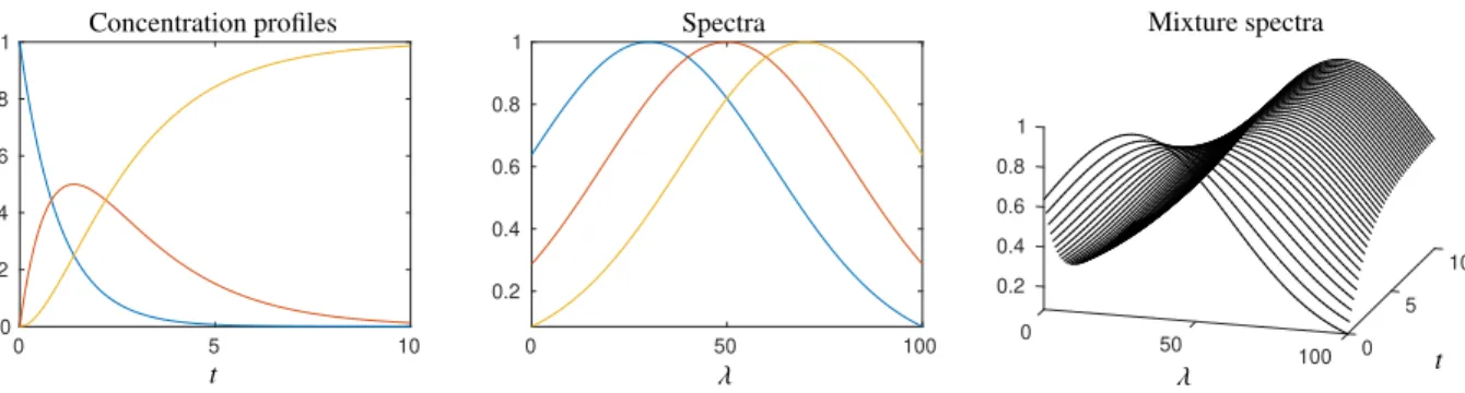
2.3. A model problem

In order to illustrate and to investigate the ambiguity measures, we take the following three-component model system. Let the consecutive reaction with the kinetic model

X−^k→¹ Y −^k→² Z

(4)

0 5 10 0

0.2 0.4 0.6 0.8 1

t

Concentration profiles

0 50 100

0.2 0.4 0.6 0.8 1

λ Spectra

10 5 0.2

0 0.4

50 0.6

0 0.8

100 1

λ t

Mixture spectra

Figure 1: The model problem as introduced in Sec. 2.3 for the parameter selectionγ=2000. Left: Concentration profiles. Center: Spectral profiles.

Right: Mixture data.

be given withk₁ =1 andk₂ =0.5. Together with the initial concentration valuesc_X(0)=1 andc_Y(0)=c_Z(0)=0 we determine the concentration factor C by solving the initial value problem. The profiles are computed on an equidistant grid withk=201 nodes andt1 =0,tk=10. The pure component spectra are computed for an equidistant discretization ofλ∈[0,100] withn=401 nodes. We use the three spectral profiles

exp

−(x−30)²/γ

, exp

−(x−50)²/γ

, exp

−(x−70)²/γ

with a parameterγ > 0. Figure 1 shows the concentration profiles definingC, the spectral profiles forγ = 2000 together with the mixture spectra, namely the rows ofD. Depending on the size of the parameterγthe AFS sets are either connected sets with a hole around the origin or can consist of three separate subsets.

2.4. Interpretation ambiguity measures for the model problem

Each of the two numbersκ1(x) andκ2(x) estimates the remaining ambiguity if a certain solutionxis fixed. Thus large valuesκ1(x) andκ2(x) mean that the remaining ambiguity is still relatively large. Contrastingly, small numbers κ1(x) respectivelyκ2(x) indicate a small remaining ambiguity. In the limit case of a unique factorization the ambiguity estimators resultκ1(x)=κ2(x)=0. However, a zero-volume AFS does not necessarily have a vanishing ambiguity, see Sec. 2.5.

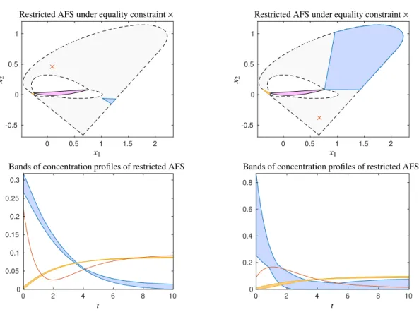
Figure 2 illustrates the AFS-restrictions by two different equality constraints for the model problem. For these two selections we observe the following:

1. An equality constraint that fixes the feasible solution with the AFS-coordinatesx=(0.086,0.458) significantly restricts the remaining ambiguity (see the two left plots). The two restricted AFS subsets are represented by a dark grey coloring. The numerical values of the ambiguity estimators areκ1 =1.046·10⁻³andκ2=0.1692.

2. Contrastingly, the feasible solutionx= (0.666,0.379) results in a weaker restriction of the AFS; see the right plots. One of the two subsets of the restricted AFS is relatively large. In other words the variability of one of the feasible concentration profiles under the given equality constraint is high. The numerical values of the estimators areκ1(x)=1.075 andκ2(x)=1.093.

It is an important fact that the ambiguity of the system under an equality constraint strongly depends on the position of the representing point of the equality constraint in the AFS. The reader can simply check and confirm these results by drawing possible Borgen triangles which include the inner polygonIS, which are also included in the outer polygon FS and for which one vertex is fixed at the point marked by anx. See [9, 10] for the geometric construction of the AFS by triangles.

2.5. Line-shaped AFS subsets and the estimatorκ1

The restrictiveness estimatorκ1(x) is computed by adding the volumes of all AFS subsets. However, a vanishing volume of an AFS subset does not guarantee the uniqueness of the associated component. Exceptions are degenerated AFS subsets, for instance line-shaped AFS subsets in the case of three-component systems or planar AFS subsets in the case of four-component systems and so on. In order to overcome the zero volume problem one might modify the estimatorκ1(x) in a way that for each subset the maximal diameter is determined and that finally all these diameters are summed up.

(5)

0 0.5 1 1.5 2 -0.5

0 0.5 1

x1

x2

Restricted AFS under equality constraint×

0 0.5 1 1.5 2

-0.5 0 0.5 1

x1

x2

Restricted AFS under equality constraint×

0 2 4 6 8 10

0 0.05

0.1 0.15 0.2 0.25 0.3

t

Bands of concentration profiles of restricted AFS

0 2 4 6 8 10

0 0.2 0.4 0.6 0.8

t

Bands of concentration profiles of restricted AFS

Figure 2: The upper row shows the AFS sets for the concentration factor of the model problem from Sec. 2.3 for the parameterγ=2000. The boundary of the original, unrestricted AFS is drawn by black broken lines. The upper left figure shows a certain fixed solution in the AFS marked by a red×symbol together with the restricted AFS (blue and ochre areas) and in the figure below the associated bounds for feasible concentration profiles. The two figures on the right show similar results for a different fixed point. The inner polygonI_S (that is uniquely determined only by the spectral mixture data matrix and does not depend on any fixed feasible solution, see [22, 26] for details on the setI_S) is drawn in light magenta in the AFS plots. The left choice of the equality constraint corresponds to a high restrictiveness (small restricted AFS), whereas the right choice results in a low restrictiveness. The areas of the bands of feasible concentration profiles determine the second estimatorκ2(x).

2.6. No quantifiable restriction for two-component systems

The application of the suggested ambiguity estimator is only useful for systems with three of more components.

The decisive point is that if for a two-component system one concentration respectively spectral profile is fixed, then this does not imply a restriction to the second concentration respectively spectral profile. (Instead, a known profile uniquely determines by duality [17, 20] a dual profile). This missing restriction can also be explained in geometrical manner. The AFS for a two-component systems consists of two intervals, one left from the origin and the other right from the origin, see [18, 22]. Then the simplex construction, which is an 1D-interval construction, satisfies forany pair of points with one pointxfrom the left interval and one pointzfrom the right interval the necessary conditions.

These conditions of the geometric AFS construction are that the interval [x,z] covers the inner polygon and that it is contained in the outer polygon.

3. Numerical results

3.1. Study of the three-component model problem

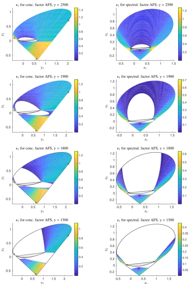
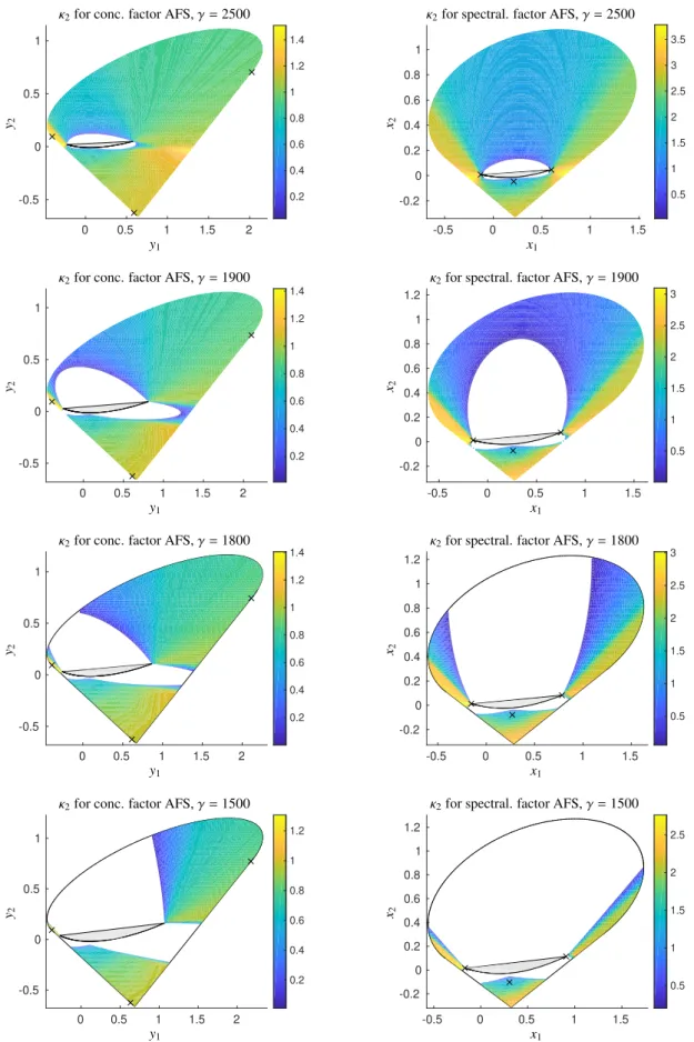
First the estimators are computed for the three-component model problem as introduced in Sec. 2.3. The concentration and spectral profiles are shown in Fig. 1 for the parameter choiceγ =2000. Next we consider the four parameter valuesγ∈ {2500,1900,1800,1500}. In the direction of fallingγwe observe a disintegration of the AFS from one connected set to three more and more isolated and smaller subsets.

Next we evaluate the ambiguity estimators not only for single points, as above, but compute the estimators for every point in the AFS. The numerical estimator values are visualized along a color coordinate. In other words, the full area of the two-dimensional AFS is colored by the values of eitherκ1orκ2. A color legend for each plot enables a size assessment of the estimator values. The resulting AFS plots have a significantly more in-depth information content compared to uniform color AFS plots. However, the computational effort is large. First, Fig. 3 shows the behavior of the AFS-volume-based ambiguity estimatorκ1for the concentration factor AFS and for the spectral factor AFS. Second, Fig. 4 shows the analogous results for the band-area-based ambiguity estimatorκ2.

(6)

0 0.5 1 1.5 2 -0.5

0 0.5 1

0.2 0.4 0.6 0.8 1 1.2 1.4

replacements

y1

y2

κ1for conc. factor AFS,γ=2500

-0.5 0 0.5 1 1.5

-0.2 0 0.2 0.4 0.6 0.8 1

0.2 0.4 0.6 0.8 1 1.2

x1

x2

κ₁for spectral. factor AFS,γ=2500

0 0.5 1 1.5 2

-0.5 0 0.5 1

0.2 0.4 0.6 0.8 1 1.2

y1

y2

-0.5 0 0.5 1 1.5

-0.2 0 0.2 0.4 0.6 0.8 1 1.2

0.1 0.2 0.3 0.4 0.5 0.6 0.7

x1

x2

κ1for spectral. factor AFS,γ=1900

0 0.5 1 1.5 2

-0.5 0 0.5 1

0.2 0.4 0.6 0.8 1 1.2

y1

y2

-0.5 0 0.5 1 1.5

-0.2 0 0.2 0.4 0.6 0.8 1 1.2

0.1 0.2 0.3 0.4 0.5 0.6

x₁ x2

0 0.5 1 1.5 2

-0.5 0 0.5 1

0.2 0.4 0.6 0.8 1

y1

y2

-0.5 0 0.5 1 1.5

-0.2 0 0.2 0.4 0.6 0.8 1 1.2

0.05 0.1 0.15 0.2 0.25 0.3 0.35 0.4

x₁ x2

Figure 3: Behavior of the AFS-volume-based ambiguity estimatorκ1for the model problem, see Sec. 3.1. Four different values of the control parameterγare used. Blue regions in these plots correspond to small values of the ambiguity estimator. Such points of the AFS are very restrictive on the remaining ambiguity if used as equality constraints. Yellow regions indicate high estimator values. The ambiguity restriction of such regions is rather low. The boundaries of the outer polygons are drawn by black lines and inner polygons are marked in a light gray; see e.g. [22, 26] for details on these polygonsF_C,F_S,I_CandI_S. The true profiles of the model problem are marked in each AFS by×symbols. The axis-scaling in the concentration factor AFS does not include the scaling by the diagonal matrixΣof singular values.

(7)

0 0.5 1 1.5 2 -0.5

0 0.5 1

0.2 0.4 0.6 0.8 1 1.2 1.4

y1

y2

-0.5 0 0.5 1 1.5

-0.2 0 0.2 0.4 0.6 0.8 1

0.5 1 1.5 2 2.5 3 3.5

x₁ x2

0 0.5 1 1.5 2

-0.5 0 0.5 1

0.2 0.4 0.6 0.8 1 1.2 1.4

y₁ y2

κ₂for conc. factor AFS,γ=1900

-0.5 0 0.5 1 1.5

-0.2 0 0.2 0.4 0.6 0.8 1 1.2

0.5 1 1.5 2 2.5 3

x1

x2

κ₂for spectral. factor AFS,γ=1900

0 0.5 1 1.5 2

-0.5 0 0.5 1

0.2 0.4 0.6 0.8 1 1.2 1.4

y₁ y2

κ₂for conc. factor AFS,γ=1800

-0.5 0 0.5 1 1.5

-0.2 0 0.2 0.4 0.6 0.8 1 1.2

0.5 1 1.5 2 2.5 3

x1

x2

0 0.5 1 1.5 2

-0.5 0 0.5 1

0.2 0.4 0.6 0.8 1 1.2

y1

y2

-0.5 0 0.5 1 1.5

-0.2 0 0.2 0.4 0.6 0.8 1 1.2

0.5 1 1.5 2 2.5

x1

x2

Figure 4: Behavior of the band-area-based ambiguity estimatorκ2for the model problem and various values of the control parameterγ. For further details and explanations on these plot see the caption of the analogous Fig. 3.

(8)

-1 -0.5 0 0.5 -0.5

0 0.5

0.1 0.2 0.3 0.4 0.5

y₁ y2

κ1for the concentration factor AFSMC

-0.5 0 0.5 1

0 0.5 1

0.2 0.4 0.6 0.8 1

x1

x2

κ₁for the spectral factor AFSM_S

-1 -0.5 0 0.5

-0.5 0 0.5

1 2 3 4

y₁ y2

κ2for the concentration factor AFSM_C

-0.5 0 0.5 1

0 0.5 1

0.5 1 1.5 2 2.5 3

x1

x2

κ₂for the spectral factor AFSM_S

Figure 5: Study of the ambiguity estimators for experimental spectral data from the hydroformylation process [12]. Upper row: The AFS-volume- based estimatorκ1for the concentration factor AFS (left) and the spectral factor AFS (right). Lower row: Behavior of the band-area estimatorκ2

for the same problem. The boundary of the outer polygons are drawn as black solid lines; all inner polygons are marked by a light gray. The six true profiles (each three concentration profiles and three spectra) are marked by×symbols.

3.2. Study of spectral data on the hydroformylation process

For this study we use experimental FT/IR spectral data gained by the rhodium catalyzed hydroformylation process;

see [12] for the experimental conditions. A number ofk=850 spectra is considered on a spectral window including absorption values forn =645 wavenumbers. Only three chemical components show a significant absorption in the selected window, namely an olefin, an acyl-complex and a hydrido-complex. The AFS for the concentration factor M_C and the AFS for the spectral factorM_S each contain three clearly separated subsets. These AFS sets together with the color coordinate on the ambiguity estimatorsκ1andκ2are plotted in Fig. 5.

3.3. Study of spectral data on a catalyst cluster formation

The chemical details on this reaction system of a rhodium catalyst cluster formation are reported in [23], wherein also a detailed chemometric analysis is presented. The data set comprisesk=290 spectra with eachn=2739 spectral channels. Three chemical components significantly absorb in the selected spectral window, namely the rhodium carbonyl clusters Rh4(CO)12 and Rh6(CO)16as well as the catalytically important species Rh(acac)(CO)2. The concentration factor AFSM_C as well as the spectral factor AFS M_S consist of three isolated subsets each. Figure 6 shows these AFS sets together with the color coordinate representation of the estimatorsκ₁andκ₂.

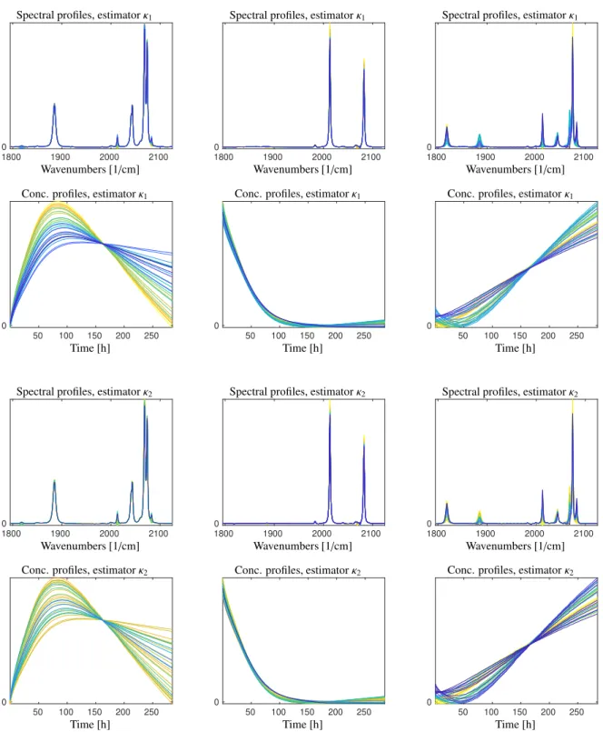
3.4. Profile-oriented visualisation of the restrictiveness

The visualization of the restrictiveness of certain profiles as illustrated by the AFS plots in Figs. 5 and 6 can be transformed to colored profiles in a band representation of the feasible bands. Next these plots are generated for the hydroformylation data and the cluster formation data. We apply the following procedure to each subset of the AFS.

First we cover the subset of the AFS with a more-or-less uniform grid. For each node of the grids we plot the feasible spectra or concentration profile in the associated color. In order to get a clear graphical presentations the number of nodes should not be to large. Maximum distinctiveness of the colored lines is achieved by using the full color spectrum with the colormap parula of Matlab. These are not exactly the same colors as in the AFS-subsets. But again, a blue profile stands for a low value of the ambiguity estimator (high restrictiveness) and a yellow profile indicates a high ambiguity estimator value (low restrictiveness). The results for hydroformylation data are shown in Fig. 7 and the results for the cluster formation data are plotted in Fig. 8.

(9)

0 1 2 3 -0.5

0 0.5

0.05 0.1 0.15 0.2 0.25 0.3

y₁ y2

κ1for the concentration factor AFSMC

0 2 4

0 0.5 1

0.1 0.2 0.3 0.4 0.5 0.6

x1

x2

κ₁for the spectral factor AFSM_S

0 1 2 3

-0.5 0 0.5

1 2 3 4

y₁ y2

κ2for the concentration factor AFSM_C

0 2 4

0 0.5 1

0.5 1 1.5 2

x1

x2

κ₂for the spectral factor AFSM_S

Figure 6: Color coordinate representation of the ambiguity estimatorsκ1 (top row) andκ2(bottom row) for the catalyst cluster formation, see Sec. 3.3. The boundaries of the outer polygons are drawn by black sold lines. The areas in light gray are the inner polygons. The chemically correct profiles are marked by×symbols. The condition numbers for the elements of the spectral AFS differ only little.

3.5. On the restrictiveness of the equality constraint and comparison of ambiguity estimation

A comparison of the numerical results for the model data and the experimental spectral data shows the following:

1. Qualitatively, the two estimatorsκ₁andκ₂produce comparable results. Regions of the AFS in which the equality constraint strongly restricts the ambiguity (this corresponds with low estimator values) are more or less the same.

This is also the case for regions with high estimator values.

This confirms the result, which is by no means self-evident, that “area” in the AFS correlates with the integral area of the feasible bands representation of rotational ambiguity. This finding underlines the close relation of the AFS approach to the feasible bands approach of Jaumot, Tauler and coworkers, see e.g. [8].

2. For the three data sets the band-area based ambiguity estimatorκ2produces results that appear to be somewhat smoother than those of the estimatorκ1. This is indicated by smoother color gradients in the estimator value plots.

3. The estimator values of eachκ1 andκ2 are monotonously decreasing on the intersection of all rays starting at the origin with the AFS. The explanation for this behavior is simple: If a feasible Borgen triangle has been constructed, then each of its vertices can be moved outwards on rays that connect the origin with the point of intersection of this ray with the boundary of the outer polygon. See also [28] for comparable ideas underlying the ray casting algorithm. Any translation of the vertex in outward direction opens additional possibilities to con- struct feasible Borgen triangles (these are triangles which include the inner polygon and which are contained in the outer polygon). The gain in feasible triangles is directly reflected by a higher rotational ambiguity (increasing estimator valueκ1) and thus also in additional feasible solutions that have the potential to broaden the feasible bands (increasing indicator valueκ2).

Conversely, equality constraints have the strongest impact on the rotational ambiguity of the restricted system if their AFS-representing points are close to the origin.

4. In general, it appears to be complex to predict the restrictiveness of an equality constraint just by knowing the boundary curves of an AFS. The ambiguity estimator values decisively depend on the form and relative orientation of the inner and outer polygons. To some extent the following holds: Equality constraints represented by points in the AFS that are close to the inner polygon along its longest main axis tend to be very restrictive on the ambiguity of the equality-restricted system - as, once again, the construction of feasible triangles is hindered by the local geometric constraints.

(10)

2000 2050 2100 0

Wavenumbers [1/cm]

Spectral profiles, estimatorκ₁

2000 2050 2100

0

Wavenumbers [1/cm]

2000 2050 2100

0

Wavenumbers [1/cm]

200 400 600 800

0

Time [min]

Conc. profiles, estimatorκ1

200 400 600 800

0

Time [min]

200 400 600 800

0

Time [min]

2000 2050 2100

0

Wavenumbers [1/cm]

Spectral profiles, estimatorκ2

2000 2050 2100

0

Wavenumbers [1/cm]

2000 2050 2100

0

Wavenumbers [1/cm]

200 400 600 800

0

Time [min]

200 400 600 800

0

Time [min]

200 400 600 800

0

Time [min]

Figure 7: Profile-oriented visualisation of the restrictiveness estimators for the hydroformylation data. The results for the ambiguity estimatorκ1

are shown in the two upper rows; the results forκ2in the two lower rows. The colors correlate with the degree of restrictiveness. The full color spectrum is used for each plot in order to attain a maximal clearness. Yellow starts with the lowest level of restrictiveness and blue ends with the highest level of restrictiveness.

(11)

1800 1900 2000 2100 0

Wavenumbers [1/cm]

1800 1900 2000 2100

0

Wavenumbers [1/cm]

1800 1900 2000 2100

0

Wavenumbers [1/cm]

50 100 150 200 250 0

Time [h]

Conc. profiles, estimatorκ₁

50 100 150 200 250

0

Time [h]

50 100 150 200 250

0

Time [h]

1800 1900 2000 2100

0

Wavenumbers [1/cm]

1800 1900 2000 2100

0

Wavenumbers [1/cm]

1800 1900 2000 2100

0

Wavenumbers [1/cm]

50 100 150 200 250 0

Time [h]

Conc. profiles, estimatorκ₂

50 100 150 200 250

0

Time [h]

50 100 150 200 250

0

Time [h]

Figure 8: Profile-oriented visualisation of the restrictiveness estimators for the cluster formation data. As in Fig. 7 the two estimatorsκ1andκ2are considered. For more details see the caption of Fig. 7.

(12)

It appears to be difficult to predict in terms of a general rule the behavior of the ambiguity estimators as shown in Figures 3 to 8. The form of the inner and outer polygons, their positions and their relative orientations are responsible for the function values of the ambiguity estimators. However, some loose rule is that all positions in the AFS that do not leave very much space for the construction of feasible triangles (including the inner polygon and being contained in the outer polygon) typically have low ambiguity estimator values. In the pure component factor construction (e.g. by the interactive tools in FACPACK) the user might start with positions with low estimator values in order to have only a low remaining ambiguity.

4. Conclusion and outlook

This paper demonstrates how an additional color coordinate can enrich the information content of AFS plots and similarly to the feasible profiles in band plots. Two estimators are studied which assign each point of the AFS a characteristic number. The estimator values can serve to measure how strongly an equality constraint fixing a point in the AFS or a profile in the bands plot can reduce the rotational ambiguity of the multivariate curve resolution (MCR) problem. We hope that this study can foster the discussion on even more general estimators of properties of the AFS and their visualization. Furthermore, we hope that the ambiguity estimators can find applications in solving practical MCR problems. The work gives some clues on how to select equality constraints so that the rotational ambiguity of the restricted system is reduced as much as possible.

In general, equality constraints are very useful for MCR computations due to their considerable impact on reducing the rotational ambiguity. In practical applications, different MCR methods have different ways to deal with equality constraints. To start with AFS-based methods, the application of an equality constraint amounts to fixing a certain point in the AFS. The impact on a reduced rotational ambiguity is geometrically understandable by the Borgen plot construction principles. Many solutions can often been ruled out as no associated Borgen triangles exist that include the inner polygon. According to our experiences such techniques work well even in the presence of a moderate level of noise since least-squares-fits typically are strong in reconstructing the major components. Sometimes data augmentation, namely an extension of the spectral mixture data by the known profile, can also be helpful. Such a procedure can (even in the case of noisy data) extend the inner polygon and simultaneously decrease the dual outer polygon (of the dual factor). These changed polygons restrict the feasible triangle constructions. Equivalently, this means that the rotational ambiguity is reduced. The process of such a data augmentation in the context of AFS constructions is for instance demonstrated in [24]. An alternative and optimization-based approach for handling equality constraints is to compute a proper matrixT for the factorsC = UΣT⁻¹ andS^T = T V^T in a way that a penalization is used for the deviation of the known profile from the factorization result. Typically this technique is effective and robust.

References

[1] H. Abdollahi and R. Tauler. Uniqueness and rotation ambiguities in multivariate curve resolution methods. Chemom. Intell. Lab. Syst., 108(2):100–111, 2011.

[2] S. Beyramysoltan, R. Rajk´o, and H. Abdollahi. Investigation of the equality constraint effect on the reduction of the rotational ambiguity in three-component system using a novel grid search method.Anal. Chim. Acta, 791(0):25–35, 2013.

[3] O.S. Borgen and B.R. Kowalski. An extension of the multivariate component-resolution method to three components. Anal. Chim. Acta, 174:1–26, 1985.

[4] P.J. Gemperline. Computation of the range of feasible solutions in self-modeling curve resolution algorithms. Anal. Chem., 71(23):5398–

5404, 1999.

[5] A. Golshan, H. Abdollahi, S. Beyramysoltan, M. Maeder, K. Neymeyr, R. Rajk´o, M. Sawall, and R. Tauler. A review of recent methods for the determination of ranges of feasible solutions resulting from soft modelling analyses of multivariate data. Anal. Chim. Acta, 911:1–13, 2016.

[6] A. Golshan, H. Abdollahi, and M. Maeder. Resolution of rotational ambiguity for three-component systems. Anal. Chem., 83(3):836–841, 2011.

[7] J. Jaumot and R. Tauler. MCR-BANDS: A user friendly MATLAB program for the evaluation of rotation ambiguities in multivariate curve resolution.Chemom. Intell. Lab. Syst., 103(2):96–107, 2010.

[8] J. Jaumot and R. Tauler. MCR-BANDS: A user friendly MATLAB program for the evaluation of rotation ambiguities in multivariate curve resolution.Chemom. Intell. Lab. Syst., 103(2):96–107, 2010.

[9] A. J ¨urß, M. Sawall, and K. Neymeyr. On generalized Borgen plots. I: From convex to affine combinations and applications to spectral data.

J. Chemom., 29(7):420–433, 2015.

[10] A. J ¨urß, M. Sawall, and K. Neymeyr. On generalized Borgen plots. II: The line-moving algorithm and its numerical implementation. J.

Chemom., 30:636–650, 2016.

[11] R. Kellner, J.-M. Mermet, M. Otto, M. Valc´arcel, and H. M. Widmer, editors.Analytical chemistry. Wiley-VCH, Weinheim, 2004.

[12] C. Kubis, M. Sawall, A. Block, K. Neymeyr, R. Ludwig, A. B¨orner, and D. Selent. An operando FTIR spectroscopic and kinetic study of carbon monoxide pressure influence on rhodium-catalyzed olefin hydroformylation. Chem.-Eur. J., 20(37):11921–11931, 2014.

[13] W.H. Lawton and E.A. Sylvestre. Self modelling curve resolution.Technometrics, 13:617–633, 1971.

[14] M. Maeder and Y.M. Neuhold.Practical data analysis in chemistry, volume 26. Elsevier, Amsterdam, 2007.

[15] E. Malinowski.Factor analysis in chemistry. Wiley, New York, 2002.

(13)

[16] K. Neymeyr, M. Sawall, and D. Hess. Pure component spectral recovery and constrained matrix factorizations: Concepts and applications.J.

Chemom., 24:67–74, 2010.

[17] R. Rajk´o. Natural duality in minimal constrained self modeling curve resolution.J. Chemom., 20(3-4):164–169, 2006.

[18] R. Rajk´o and K. Istv´an. Analytical solution for determining feasible regions of self-modeling curve resolution (SMCR) method based on computational geometry.J. Chemom., 19(8):448–463, 2005.

[19] C. Ruckebusch and L. Blanchet. Multivariate curve resolution: A review of advanced and tailored applications and challenges. Anal. Chim.

Acta, 765:28–36, 2013.

[20] M. Sawall, C. Fischer, D. Heller, and K. Neymeyr. Reduction of the rotational ambiguity of curve resolution techniques under partial knowledge of the factors. Complementarity and coupling theorems.J. Chemom., 26:526–537, 2012.

[21] M. Sawall, A. J ¨urß, H. Schr¨oder, and K. Neymeyr.On the analysis and computation of the area of feasible solutions for two-, three- and four- component systems, volume 30 of Data Handling in Science and Technology, “Resolving Spectral Mixtures”, Ed. C. Ruckebusch, chapter 5, pages 135–184. Elsevier, Cambridge, 2016.

[22] M. Sawall, A. J ¨urß, H. Schr¨oder, and K. Neymeyr. Simultaneous construction of dual Borgen plots. I: The case of noise-free data.J. Chemom., 31:e2954, 2017.

[23] M. Sawall, C. Kubis, E. Barsch, D. Selent, A. B¨orner, and K. Neymeyr. Peak group analysis for the extraction of pure component spectra.J.

Iran. Chem. Soc., 13(2):191–205, 2016.

[24] M. Sawall, C. Kubis, H. Schröder, D. Meinhardt, D. Selent, R. Franke, A. Brächer, A. Börner, and K. Neymeyr. Multivariate curve resolutions methods and the design of experiments.J. Chemom., 2019. Accepted for publication.

[25] M. Sawall, C. Kubis, D. Selent, A. B¨orner, and K. Neymeyr. A fast polygon inflation algorithm to compute the area of feasible solutions for three-component systems. I: Concepts and applications.J. Chemom., 27:106–116, 2013.

[26] M. Sawall, A. Moog, C. Kubis, H. Schröder, D. Selent, R. Franke, A. Brächer, A. Börner, and K. Neymeyr. Simultaneous construction of dual Borgen plots. II: Algorithmic enhancement for applications to noisy spectral data.J. Chemom., 32:e3012, 2018.

[27] M. Sawall and K. Neymeyr. A fast polygon inflation algorithm to compute the area of feasible solutions for three-component systems. II:

Theoretical foundation, inverse polygon inflation, and FAC-PACK implementation.J. Chemom., 28:633–644, 2014.

[28] M. Sawall and K. Neymeyr. A ray casting method for the computation of the area of feasible solutions for multicomponent systems: Theory, applications and FACPACK-implementation. Anal. Chim. Acta, 960:40–52, 2017.

[29] R. Tauler. Calculation of maximum and minimum band boundaries of feasible solutions for species profiles obtained by multivariate curve resolution.J. Chemom., 15(8):627–646, 2001.

[30] M. Vosough, C. Mason, R. Tauler, M. Jalali-Heravi, and M. Maeder. On rotational ambiguity in model-free analyses of multivariate data.J.

Chemom., 20(6-7):302–310, 2006.