How can we understand the global distribution of the solar cycle signal on the Earth’s surface?

(1)

www.atmos-chem-phys.net/16/12925/2016/

doi:10.5194/acp-16-12925-2016

How can we understand the global distribution of the solar cycle signal on the Earth’s surface?

Kunihiko Kodera¹, Rémi Thiéblemont², Seiji Yukimoto³, and Katja Matthes^4,5

1Institute for Space-Earth Environmental Research, Nagoya University, Nagoya, 464-8601, Japan

2Laboratoire Atmosphères Milieux Observations Spatiales, 78280 Guyancourt, France

3Meteorological Research Institute, Tsukuba, 305-0052, Japan

4Research Division Ocean Circulation and Climate, GEOMAR Helmholtz Centre for Ocean Research, 24105 Kiel, Germany

5Christian-Albrechts Universität zu Kiel, 24105 Kiel, Germany Correspondence to:Kunihiko Kodera (kodera@isee.nagoya-u.ac.jp)

Received: 13 February 2016 – Published in Atmos. Chem. Phys. Discuss.: 25 February 2016 Revised: 12 September 2016 – Accepted: 28 September 2016 – Published: 19 October 2016

Abstract. To understand solar cycle signals on the Earth’s surface and identify the physical mechanisms responsible, surface temperature variations from observations as well as climate model data are analysed to characterize their spatial structure. The solar signal in the annual mean surface temperature is characterized by (i) mid-latitude warming and (ii) no overall tropical warming. The mid-latitude warming during solar maxima in both hemispheres is associated with a downward penetration of zonal mean zonal wind anomalies from the upper stratosphere during late winter. During the Northern Hemisphere winter this is manifested by a modulation of the polar-night jet, whereas in the Southern Hemi- sphere, the upper stratospheric subtropical jet plays the ma- jor role. Warming signals are particularly apparent over the Eurasian continent and ocean frontal zones, including a previously reported lagged response over the North Atlantic. In the tropics, local warming occurs over the Indian and central Pacific oceans during high solar activity. However, this warming is counterbalanced by cooling over the cold tongue sectors in the southeastern Pacific and the South Atlantic, and results in a very weak zonally averaged tropical mean signal.

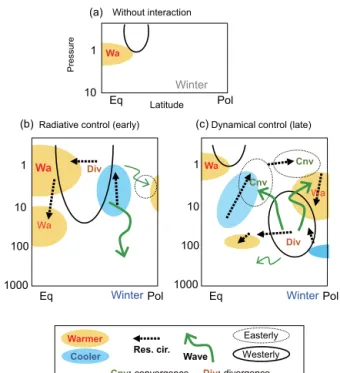
The cooling in the ocean basins is associated with stronger cross-equatorial winds resulting from a northward shift of the ascending branch of the Hadley circulation during solar maxima. To understand the complex processes involved in the solar signal transfer, results of an idealized middle atmosphere–ocean coupled model experiment on the impact of stratospheric zonal wind changes are compared with solar signals in observations. Model integration of 100 years of

strong or weak stratospheric westerly jet condition in winter may exaggerate long-term ocean feedback. However, the role of ocean in the solar influence on the Earth’s surface can be better seen. Although the momentum forcing differs from that of solar radiative forcing, the model results suggest that stratospheric changes can influence the troposphere, not only in the extratropics but also in the tropics through (i) a downward migration of wave–zonal mean flow interactions and (ii) changes in the stratospheric mean meridional circulation.

These experiments support earlier evidence of an indirect solar influence from the stratosphere.

1 Introduction

The influence of solar activity on the Earth’s surface, espe- cially that of the 11-year solar cycle, has been debated for a long time (e.g. Pittock, 1978; Legras, 2010). The climate impact of solar influence is generally assessed in terms of the radiative forcing (e.g. IPCC, 2013). Recent direct measure- ments from space reveal that changes in the total solar irradiance (TSI) associated with the 11-year solar cycle are about 0.1 % (1.3 W m⁻²)(Kopp and Lean, 2011). Such small variations are not expected to have a significant impact on surface climate, and so several mechanisms have been proposed that act to amplify the initially small solar effects. One amplification mechanism is the enhancement of the direct TSI effect at the ocean surface due to a feedback of water vapour transport in the tropical Pacific (Meehl et al., 2008, 2009). Another

(2)

possible amplification mechanism works through a change in the solar spectrum, in particular in the ultraviolet (UV) range, directly affecting the stratopause region and enhanc- ing temperatures and ozone concentrations during the solar cycle. The amplification and the downward penetration of the small initial solar signal occur through stratospheric dynamical processes (e.g. Kodera and Kuroda, 2002). The impact of cosmic rays on surface temperature through changes in cloud cover has also been proposed (Svensmark and Friis- Christensen, 1997).

Besides an apparently small direct solar effect, another problem of explaining solar influence on climate is the rather unstable relationship between the 11-year solar cycle and the Earth’s global mean surface temperature, as a break- down or even the reversal of the relationship occurs during different time periods (e.g. Nitta and Yoshimura, 1993;

Georgieva et al., 2007; Souza-Echer, 2012). However, Zhou and Tung (2010) extracted a global spatial pattern of sea surface temperature (SST) variations associated with the solar cycle by applying a composite mean difference (CMD) pro- jection method, particularly relevant to estimate the robust- ness of a global spatial signal. This method segregates data into groups of high and low solar activity during the 11-year cycle. A global spatial pattern is then obtained from the composite mean difference between the high and low solar group.

Finally, the original data are projected onto this CMD spatial pattern, resulting in a time series. The method is successful when the correlation between the resulting time series and the solar forcing is high. They demonstrated that the coefficients of this CMD pattern projected onto the global SST field show a steady and highly robust relationship with the solar activity over more than 10 solar cycles (represented by the TSI for the past 153 years reconstructed by Y.-M.

Wang et al., 2005). This indicates that a global spatial pattern, rather than a globally averaged temperature, is crucial to understanding solar influences at the surface.

Various studies of the solar influence on weather and climate were reviewed by Gray et al. (2010). Here, we do not attempt to extensively review previous works, but rather look for consistent aspects of the solar signals reported in many independent studies. The surface response to solar forcing is regionally distributed; that means that the solar signal is influenced by the internal dynamics of the climate system.

Our paper aims to suggest supplementary physical processes that may help to better understand the global distribution of the solar signal. In the following, we will particularly show that the atmosphere–ocean interactions may play an important role in determining surface solar signal over baroclinic zones and tropical cold tongue regions.

Surface temperature and pressure have been measured for more than 100 years. Thus, the relationship between surface temperature variations and solar activity can be investigated using a global historical dataset. Because sea surface temperature (SST) is more persistent than the sea-level pressure, long-term variations can be more easily detected in the tem-

perature field. Therefore, we investigate mainly surface temperature variation from the historical data, complemented by pressure or geopotential height fields with a modern dataset.

Direct measurement of the solar UV is only recent, but a record of the sunspot number, which is a proxy of the solar extreme ultraviolet (EUV), is available from the 18th century. The solar EUV produces the ionization in the Earth’s upper atmosphere. Therefore, change in the solar EUV radiation is felt on the Earth’s surface as change in geomagnetic field induced by the electric current in the ionosphere. It is, thus, possible to associate the variation of sunspot number with the solar EUV activity. Comparison of the variation calculated from Earth’s magnetic field demonstrates excellent agreement between the 10.7 cm solar radio flux (F10.7) and the sunspot number (Svalgaard, 2007). Therefore, both can be used as a proxy of the solar irradiance variation.

Annual mean surface temperature anomalies related to the solar cycle have been studied using various methods and different historical global datasets covering between 120 and 150 years. Lohmann et al. (2004) calculated the correlation coefficient between the proxy solar irradiance from Lean et al. (1995) and band-pass (between 9- and 5-year period) filtered SSTs reconstructed by Kaplan et al. (1998) from 1856 to 2000. Lean and Rind (2008) extracted solar signals by applying a multiple linear regression analysis to surface temperatures reconstructed by the University of East Anglia Climatic Research Unit F (Brohan et al., 2006) for the period 1889–2006. A similar multiple linear regression analysis was conducted by Tung and Zhou (2010), who compared the regression analysis of two different historical datasets, namely NOAA’s Extended Reconstructed Sea Sur- face Temperatures (ERSST) and the Hadley Centre Sea Ice and Sea Surface Temperature (HadISST) dataset (Rayner et al., 2003), to confirm consistent features of the solar signal.

Gray et al. (2013) performed a lagged multiple linear regression analysis to investigate delayed components in the solar signal using the HadISST dataset. Despite different recon- structions and analysis methods, common features are seen during high solar activity in the surface temperatures: a mid- latitude warming, and a tropical cooling in the southeastern Pacific and the South Atlantic. Note that this cooling is different from the La Niña-like pattern previously reported (van Loon et al., 2007; Meehl et al., 2008, 2009) and will be discussed in more detail below.

We first compare the analysis results of a historical surface temperature dataset with those of a modern dataset to identify the fundamental global features of surface temperature variations related to the solar cycle, i.e. the observed surface solar signals. Next, we study the vertical structure of the solar signal with recent data to identify possible physical mechanisms producing the surface solar signals. Identi- fication of the causes and characteristics of solar signals is particularly difficult for decadal-scale periodic variations because strong feedbacks exist on these timescales in the climate system. To better understand the mechanisms produc-

(3)

ing the surface solar signal, we revisit results from an idealized middle atmosphere–ocean coupled general circulation experiment where a momentum forcing has been applied in the stratosphere (Yukimoto and Kodera, 2007).

The remainder of this paper is organized as follows. After describing the data and method of analysis in Sect. 2, characteristics of the solar signal in atmospheric as well as oceanic variables are described in Sect. 3. To understand the complex processes for the solar signal transfer involving stratosphere–

troposphere–ocean coupling, results of an idealized numeri- cal experiment are compared with observed solar signals in Sect. 4. To get insight into a centennial solar variation such as the Maunder Minimum, the effect of centennial-scale stratospheric circulation changes on the troposphere is briefly studied in Sect. 5. Finally, discussions and a summary about the possible mechanisms producing the solar influence on the Earth’s surface are given in Sect. 5.

2 Data and analysis 2.1 Data

This study combines the analysis of a historical SST dataset to characterize the surface response to the 11-year solar cycle, with a modern reanalysis dataset to investigate the underlying dynamical processes. For the historical dataset, we use the NOAA Extended Reconstructed SST v3b (ERSST), described by Smith et al. (2008) and available at http://www.esrl.noaa.gov/psd/data/gridded/data.noaa.

ersst.html. The ERSST dataset spans more than 160 years from 1854 to the present, with monthly resolution, and a spatial resolution of 2^◦ longitude×2^◦ latitude from 88^◦N to 88^◦S and 0 to 358^◦E. Given the sparsity of observations before 1880 (Smith and Reynolds, 2003), we limited the present study to the period 1880–2010. To examine the tropospheric and stratospheric dynamical response to the solar cycle, we use the ERA-Interim atmospheric reanalysis produced by the European Centre for Medium-Range Weather Forecasts (ECMWF) (Dee et al., 2011). We used the ERA- Interim (ERA-I) dataset from 1 January 1979 to 2010. In this study, we used monthly mean data, provided on 23 pressure levels from 1000 to 1 hPa with a spatial resolution of 2.5^◦ longitude×2.5^◦latitude.

2.2 Multiple linear regression model

Following numerous earlier studies (e.g. Lean and Rind, 2008; Frame and Gray, 2010; Chiodo et al., 2014; Mitchell et al., 2015a, b), the ocean and atmosphere responses to solar variations are examined using a multiple linear regression (MLR) model. This technique can isolate the effects of different forcings, represented by explanatory variables (or regressors), on the variance of a time-dependent variable (or predictand). Annual signals are extracted by applying the MLR to continuous monthly resolved time series. Monthly or sea-

sonal signals (2 to 3 consecutive months) are diagnosed by applying the MLR to time series of the individual month or season (i.e., the seasonal average is performed prior to the MLR), respectively. All data time series have the seasonal cycle removed before the MLR, as well as before any seasonal- average calculations.

The MLR model is applied at each location and is given by

X (t )=A·CO2(t )+B·N3.4(t )+C·F10.7(t−1t ) +D·AOD(t )+E·QBOa(t )+F·QBOb(t )+(t ), (1)

whereX(t) is the time-dependent variable, the first six terms on the right-hand side of the equation correspond to the prod- uct of one time-dependent explanatory variable (e.g. CO2(t )) and its regression coefficient (e.g.A) and the last termε(t )is the residual error.

The explanatory variables considered for the MLR de- scribe variability sources that are demonstrated to have a significant impact on the surface, troposphere and middle atmosphere dynamics, and have been broadly used in solar- climate studies based on model and reanalysis (e.g. Chiodo et al., 2014; Mitchell et al., 2015a, b). The explanatory variables are defined as follows: the CO₂concentration (Meinshausen et al., 2011) (available at http://climate.uvic.ca/EMICAR5/

forcing_data/RCP85_MIDYR_CONC.DAT) to account for the increase in anthropogenic forcing; the Niño 3.4 index derived from the ERSST v3b dataset; the F10.7 cm solar radio flux index (available at http://lasp.colorado.edu/lisird/tss/

noaa_radio_flux.html); and the global aerosol optical depth (AOD) at 550 nm updated from Sato et al. (1993) to represent volcanic effects and two stratospheric quasi-biennial oscillation (QBO) orthogonal indices (QBOa and QBOb), defined as the first two principal components of the ERA-I zonal mean zonal wind in the latitude interval (10^◦S, 10^◦N) and pressure–height interval (70–5) hPa, respectively.

QBO regressors and F10.7 index are only available from the mid-20th century, so that QBO regressors are not in- cluded in the MLR and the F10.7 index is replaced by the sunspot numbers when the long-term historical SST dataset is analysed. Sensitivity tests of the MLR model revealed that including or removing the stratospheric QBO regressors for the period 1979–2010 negligibly affects the solar regression coefficients and their statistical significance, in particular in the troposphere. Although the F10.7 cm index more directly represents the irradiance variability in the UV band than the sunspot number (Tapping, 2013), both indices concur at annual timescales: a correlation coefficient of 0.997 between the annually averaged F10.7 and sunspot number time series is found for the period 1965–2012. The solar regression coefficient used in our study assumes that a difference of 130 solar flux units (1 sfu=10⁻²²W m⁻²Hz⁻¹)or 100 sunspots represents the difference between the 11-year solar cycle maximum and minimum.

(4)

To investigate the effect of the ocean memory on the surface response to solar variability (e.g. Gray et al., 2013;

Thiéblemont et al., 2015), we calculated the MLR at different time lags (1tin months or years) with respect to the solar regressor. The Arctic Oscillation (AO) or the North Atlantic Oscillation (NAO) is a climate mode of variability, which is partly driven by solar variability as will be shown later.

Hence, it is not appropriate to include its index in an MLR model, which aims to examine the solar cycle effect on surface climate.

When applying regression techniques, it is essential to carefully consider possible autocorrelation in the residual to assess statistical significance of the regression coefficients.

Autocorrelation in the residual leads to an underestimation of the regression coefficient uncertainties, and thus a nar- rowing of the confidence intervals. A common method em- ployed to circumvent the residual autocorrelation problem is to treat the residual term as an autoregressive process (Tiao et al., 1990). The first step of the procedure, also called prewhitening, consists of correcting both the predictors and the predictand (X)with the autocorrelation coefficient of the residual term estimated from a first application of the regression model. The prewhitening procedure is then repeated on the modified predictors and predictand until the residual is no longer significantly autocorrelated. The statistical significance of the autocorrelation is assessed with a Durbin–

Watson test. The application of the Tiao et al. method can be found in several papers examining the solar signal (e.g.

Austin et al., 2008; Mitchell et al., 2015b). We generally found that a single application of the prewhitening procedure was sufficient to remove the residual autocorrelation al- most completely (more than 95 % of the grid points). Once the prewhitening step has been performed, the statistical significance of the regression coefficients is calculated using a two-tailed Student’sttest.

The use of the MLR approach to separate the contribu- tion of different factors to climate variability has inherent limitations that should be kept in mind when analysing the results. The MLR particularly relies on several assumptions that may not be valid in all cases. However, composite analysis of the monthly mean data based on high and low levels of solar activity (e.g. Kuroda and Kodera, 2002; Lu et al., 2011) also produces similar solar signals as those obtained from the MLR method (Figs. 6, 7). Therefore, in spite of the limitations, the MLR method may be useful to get approxi- mate solar signals (Kuchar et al., 2015). We note that highly non-linear responses can be produced through the interaction between different forcings: for example, between El Niño–

Southern Oscillation (ENSO) and solar signals (Marsh and Garcia, 2007), solar and QBO signals (Matthes et al., 2013), as well as volcanic and solar signals (Chiodo et al., 2014).

Usually this kind of interaction occurs at a specific location and time, which needs to be investigated in separate studies.

Sophisticated attribution methods that can account for non- linearity have been used, such as machine learning methods

(Blume et al., 2012) or optimal detection (Stott et al., 2003;

Mitchell, 2016). Although these methods use advanced statistical techniques, it is difficult to relate the conclusions to specific physical mechanisms.

3 Solar signal

3.1 Surface temperature signal

As mentioned in the Introduction, Zhou and Tung (2010;

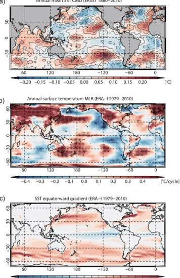
hereafter ZT2010) calculated CMDs between high- and low- activity periods of the 11-year solar cycle using the ERSST dataset. In their analysis, data near the World War II period (1942–1950) were excluded. We performed the same CMD analysis using the same dataset as ZT2010, but starting in 1880 instead of 1854. We confirm the results of ZT2010 in Fig. 1a. The correlation coefficient between the expansion coefficients of the extracted pattern and the solar index shows a similar high correlation (0.69).

To assess the stability of the relationship between SSTs and the solar cycle, the use of a long dataset is crucial. How- ever, historical datasets have problems with spatial cover- age and inhomogeneity of the observing systems. This draw- back may be compensated by a comparison with a recent global dataset assimilating satellite observations. Figure 1b shows the surface solar signal extracted by MLR using the ERA-I and F10.7 cm radio flux time series (solar index) as one of the explanatory variables for the period from 1979 to 2010. Despite the short time period of only three solar cycles, the results show a similar pattern in surface temperature to those obtained from longer historical datasets. Common features in the spatial structure of the solar signal in surface temperatures include (i) (subpolar regions): warming around 45–60^◦N over the Eurasian continent and cooling over the west of Greenland; (ii) (mid-latitudes): warming over the ocean basins around 30–45^◦latitudes in the Northern Hemi- sphere (NH) as well as in the Southern Hemisphere (SH);

(iii) (tropics): warming over the Indian Ocean and the central Pacific, and cooling in the eastern Pacific and the Atlantic, particularly in the SH. These characteristics are also found in a number of other studies, cited in the Introduction, that use different analysis techniques. In spite of overall similari- ties, large differences can be found in some regions, such as over the subtropical eastern Pacific, east of Hawaii. It shows large warming in the historical data (Fig. 1a), but cooling in the modern era data (Fig. 1b). It is, however, difficult to identify whether the difference in short-term data is merely due to statistical fluctuations, or related to a change in basic climatological states caused by other factors, such as global warming or ocean circulation change. Here, we concentrate on the stable solar response to first understand how it is produced at the Earth’s surface. To investigate the solar signals over the ocean basins specifically, equatorward gradients of climatological SSTs are shown in Fig. 1c. The regions where warming during solar maxima occurs roughly correspond to

(5)

60 120 180 −120 −60 0

−60−3003060

−0.4 −0.3 −0.2 −0.1 0.0 0.1 0.2 0.3 0.4 [^OC/cycle]

Annual surface temperature MLR (ERA−I 1979−2010)

60 120 180 −120 −60 0

−60−3003060

−0.4 −0.3 −0.2 −0.1 0.0 0.1 0.2 0.3 0.4 [^OC/100 km]

SST equatorward gradient (ERA−I 1979−2010)

c ( ) (b) (a)

−0.20 −0.15 −0.10 −0.05 0.00 0.05 0.10 0.15 0.20 [^OC]

Annual mean SST CMD (ERSST 1880−2010)

60 120 180 −120 −60 0

−30030

Figure 1.T (a)Annual mean SST anomaly extracted by the same CMD analysis as in Zhou and Tung (2010) for the period 1880–

2010.(b)Annual solar index regression coefficient of the surface temperature derived by applying the MLR model to ERA-I data for the period 1979–2010. Stippled areas indicate statistical significance at the 95 % level.(c)Equatorward gradient of annual mean climatological SST.

regions of strong meridional SST temperature gradients. The case of solar signals over the North Atlantic frontal zone is more complicated (see Fig. 1a), and in fact solar signals over the North Atlantic are delayed by about 3 years (Gray et al., 2013; Scaife et al., 2013; Andrews et al., 2015; Thiéblemont et al., 2015), and will be discussed later. Note also that regions with cool solar signals in the tropics coincide with sectors of the cold tongue over the equatorial eastern Pacific and the Atlantic. This kind of temperature pattern is quite different from the expected impact of TSI variations from an energy balance model. Stevens and North (1996) estimated a warming in the tropics from such a model, in particular over the continents.

To identify the physical mechanisms responsible for the surface solar signals, a comparison of the surface temper-

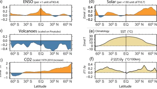
ature pattern associated with other forcings has been performed similarly to Lean and Rind (2008). The zonal mean surface temperature pattern extracted by an MLR is shown in Fig. 2. In the MLR model of Lean and Rind (2008), who used historical data, anthropogenic forcing combines anthropogenic aerosol and greenhouse gases effects. Although their anthropogenic signal shows a rather uniform warming latitu- dinally that differs from that of the present study, the other signals (i.e. ENSO, volcanic and solar) are similar. ENSO- related temperature variations (Fig. 2a) are confined to the tropics. The response to volcanic aerosol (Fig. 2b) is a global cooling, whereas the response to anthropogenic greenhouse gas forcing (Fig. 2c) is characterized by a large warming in the polar region of the NH. A cooling trend is also found in the Southern Ocean around 60^◦S. However, it could also re- sult from ozone depletion (Thompson et al., 2011) because trends in CO₂and ozone concentration cannot be well sepa- rated due to the short analysis period. The solar signal is large in mid-latitudes in both hemispheres (Fig. 2d) as already reported in Lean and Rind (2008). The reason for such a latitudinal distribution has not been addressed, however. If the surface solar signal originates from the absorption of the solar energy at the Earth’s surface, we should expect a higher solar signal in the tropics similar to the climatological SST distribution (Fig. 2e). However, a large solar signal is observed in the frontal zones where the meridional gradient of surface temperature is the largest (Fig. 2f) and where the interaction between the atmosphere and the ocean is particularly strong (Nakamura et al., 2008). This suggests, thus, a possible role of atmosphere–ocean interaction in the baroclinic zone in the modulation and amplification of the solar signal.

To explain solar signals at the surface in high latitudes, the role of the annular mode (AM) (Thompson and Wallace, 2000) in the NH (NAM) in mediating tropospheric solar signals has been suggested (e.g. Baldwin and Dunkerton, 2005).

The AM in the SH is called the SAM. However, in the SH, Lu et al. (2011) found little relationship between the solar cycle and the SAM on the surface. The surface signal of NAM and SAM are also called Arctic Oscillation (AO) and Antarc- tic Oscillation (AAO), respectively. The question we address here is the role of AM in a global perspective: how does the solar signal comparatively manifest in the SH and in the NH?

Figure 3 compares solar signals with annular modes in the two hemispheres. In NH winter (DJF), solar signals exhibit a similar pattern to the NAM: a warming over the Eurasian continent and the ocean basins along 30–45^◦N latitudes, and a cooling west of Greenland. Stronger westerly winds associated with the NAM and surface solar signals occur at lower latitudes over the American continent than over the Eurasian continent. This means that the NAM is not strictly annular, but also contains a stationary planetary wave structure. It should be noted that the spatial pattern of the solar signal is similar to that of the NAM. In SH spring (SON), solar signals are characterized by a warming in mid-latitudes associated with anomalous westerlies around 40–50^◦S. However, the

(6)

−0.2 0.0 0.2 0.4

Solar (per +130 unit of f10.7)

−0.4

−0.2 0.0 0.2

Volcanoes (scaled on Pinatubo)

−0.2 0.0 0.2 0.4

ENSO (per +1 unit of N3.4)

−1 0 1 2

CO2 (scaled 1979-2010 increase)

−10100 20 30

SST (°C)

−0.2 0.0 0.2 0.4

∂ SST/∂y (°C/100km)

Latitude Latitude

Zonal ΔTZonal T∂T/∂y Zonal ΔTZonal ΔTZonal ΔT

(d)

(c) (b) (a)

(e)

(f)

Zonal mean surface temperature (1979–2010)

Climatology

60º S 30º S EQ 30º N 60º N

Figure 2.MLR analysis of the annual zonal mean surface temperature from ERA-I, calculated for the period 1979–2010, for(a)ENSO, (b)volcanic activity and(c)CO₂concentration, and(d)solar activity. Climatological zonal mean SSTs and their equatorward meridional gradient are also shown in(e)and(f), respectively.

60 120 180 −120 −60 0

3040506070

−0.8 −0.6 −0.4 −0.2 0.0 0.2 0.4 0.6 0.8 (f) AO T1000

60 120 180 −120 −60 0

3040506070

−0.8 −0.6 −0.4 −0.2 0.0 0.2 0.4 0.6 0.8 (e) AO U500

60 120 180 −120 −60 0

−70−60−50−40−30

−0.8 −0.6 −0.4 −0.2 0.0 0.2 0.4 0.6 0.8 (g) AAO U500

60 120 180 −120 −60 0

−70−60−50−40−30

−0.8 −0.6 −0.4 −0.2 0.0 0.2 0.4 0.6 0.8 (h) AAO T1000

Solar cycle ^1979–2010 Annular modes

SH (SON) NH (DJF)

60 120 180 −120 −60 0

3040506070

−2.4 −1.8 −1.2 −0.6 0.0 0.6 1.2 1.8 2.4 [ms⁻¹/cycle]

60 120 180 −120 −60 0

3040506070

−1.6 −1.2 −0.8 −0.4 0.0 0.4 0.8 1.2 1.6 [^OC/cycle]

60 120 180 −120 −60 0

−70−60−50−40−30

−0.8 −0.6 −0.4 −0.2 0.0 0.2 0.4 0.6 0.8 [^OC/cycle]

60 120 180 −120 −60 0

−70−60−50−40−30

−2.4 −1.8 −1.2 −0.6 0.0 0.6 1.2 1.8 2.4 [ms⁻¹/cycle]

(c) Solar U500

(d) Solar T1000 (a) Solar U500

(b) Solar T1000

Figure 3.Solar regression coefficient extracted by the MLR technique for the DJF mean NH(a)500 hPa zonal mean wind, and(b)surface temperature. Panels (candd): same as (aandb), but for the SON mean in the SH. Panels (eand f): same as (aandb), except for the correlation with surface NAM index. Panels (gandh): same as (candd), except for the surface SAM index. The period of analysis is 1979–2010. Stippled regions with black and white dots indicate statistical significance at the 90 and 95 % level, respectively.

(7)

100 10 1

−80 −70 −60 −50 −40 −30 −20

100 10 1

Latitude [ N]^O

Pressure [hPa]

100 10 1

20 30 40 50 60 70 80

100 10 1

Latitude [ N]^O

Pressure [hPa]

(a) June SH (b) December NH

−0.4 −0.3 −0.2 −0.1 0.0 0.1 0.2 0.3 0.4 [ K 100 km ]⁻¹

Figure 4.Meridional sections of the climatological poleward temperature gradient around the winter solstice:(a)SH June,(b)NH December.

SAM pattern typically involves a strong warming around the Antarctic Peninsula and the southern tip of the South Amer- ican continent (Thompson and Wallace, 2000; Gillett et al., 2006) in association with anomalous westerlies near the polar region around 55–65^◦S. This is the reason why solar signals are not projected to the SAM in the SH, unlike to the NH.

3.2 Zonal mean vertical structure

Since the surface solar signals during the recent (1979–2010) period is very similar to that of the longer historical period (1880–2010) (Fig. 1), we may gain further insight into the processes responsible for the solar signal transfer from the stratosphere to the troposphere and the ocean by analysing the modern dataset in more detail. First of all, it should be noted that there are two kinds of westerly jets in the middle atmosphere. Climatological poleward temperature gradient during winter solstice (June in the SH, and December in the NH) is displayed in Fig. 4. The meridional temperature gradient is large in the subtropics of the upper stratosphere due to solar UV heating, while in the lower stratosphere, the gradient is strong around the polar-night region due to longwave cooling. They are respectively connected to the subtropical and polar-night jet. From this, we can expect that the variation in the solar UV heating first manifests in the subtropics of the stratopause region.

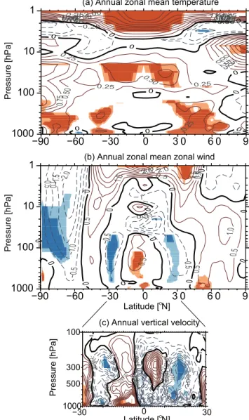
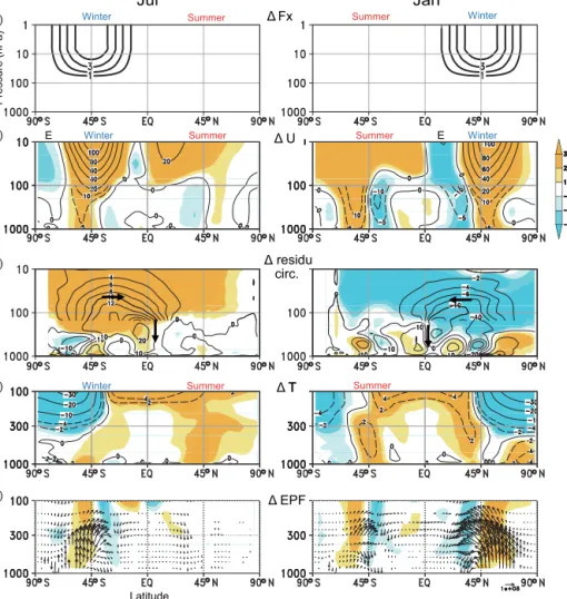
Figure 5 shows solar signals in the annual mean (a) zonal mean zonal wind, (b) zonal mean air temperature and (c) pressure coordinate vertical velocity in the tropical troposphere using the same MLR analysis as in Fig. 1b. The results of similar MLR analyses using meteorological reanalysis data have also been published (e.g. Frame and Gray, 2010;

Chiodo et al., 2014; Mitchell et al., 2015a). During periods of high solar activity, warming signals appear at three levels: the upper stratosphere–stratopause (5–1 hPa), the lower to middle stratosphere (100–20 hPa) and the troposphere (1000–

300 hPa) (Fig. 5a). The warming around the stratopause ex- tends globally from the tropics to the polar regions, while the warming in the lower stratosphere is confined to the trop-

0.25 0.25

0.25

0.25 0.25

0.25

0.50 0.50

0.50

0.50 0.50

0.75 0.75

0.75

1.00

1.00 1.25

1.251.75 2.002.251.50 1.501.752.002.25

−0.50

−0.25

−0.25 0

0 0

0

0 0 0

0

1000 100 10 1

−90 −60 −30 0 3 0 6 0 9 0

0.5

0.5 0.5

0.5

0.5 1.0 1.0

1.0

2.0 1.5

2.53.0

−1.5 −2.0

−1.0

−0.5

0 0

0

0 0

0 0 0

0

0 0

0

1000 100 10 1

−90 −60 −30 0 3 0 6 0 9 0

1.50•10−4

1.50•10

−4

3.00•10⁻⁴ 3.00•10

−4

3.00•10

−4 −9

.00•10

−4−9.00•10

−4 −7.50•10

−4

−7.50•10

−4

−6.00•10

−4−6.00•10

−4−4.50•10−4 −4.50•10

−4

−3.00•1 0

−4

−3.00•10−4

−3.00•10

−4

−1.50•10

−4

−1.50•

−410

−1.50•10

−4

−1.50•10

−4

0

00 0

0 0 0

0

1000 500 300 100

−30 30

(a) Annual zonal mean temperature

(b) Annual zonal mean zonal wind

O

(c) Annual vertical velocity Pressure [hPa]Pressure [hPa] Pressure [hPa]

Latitude [ N]^O

Latitude [ N]0 ^O

Figure 5.Solar regression coefficients of the annual zonal mean (a)air temperature,(b)zonal wind and(c)vertical velocity in the tropical troposphere. Solid (dashed) contours indicate positive (negative) values and are drawn every(a)0.25 K, (b) 0.5 m s⁻¹ and (c)5 m day⁻¹. Areas of 90 and 95 % statistical significance are shown by light and dark shading, respectively, in red (positive) and blue (negative).

ics. The associated stronger meridional temperature gradient in the subtropical upper stratosphere is connected, by the thermal–wind relationship, to enhanced subtropical jets around 30–40^◦ latitude in both hemispheres in the upper stratosphere (Fig. 5b). Stronger subtropical jets extend far- ther to lower altitudes in association with a warming in the tropical lower stratosphere. The narrow latitudinal extent of the zonal mean zonal wind anomalies at mid-latitudes of the middle–lower stratosphere in Fig. 5 is difficult to explain only from a radiative heating change. The differences in the latitudinal structure of the warming suggest that the warming in the stratopause–upper stratosphere has a radiative origin,

(8)

−2

−1

1 1 246 108

0 0

0

1 10 100 1000

Pressure (hPa)

Jul

−4−2−1

1 246 0 8

0 0

0 0 1

10 100 1000

Pressure (hPa)

Aug

−4

−1−2 −1 −1 12

0 ₀

1 10 100 1000

Pressure (hPa)

Sep

−2 −4

−1

0 0

1 10 100 1000

Pressure (hPa)

Latitude

Oct

1 1 2 2 4 6

0 0

Nov

−4−2−1

1 1 24

6 0

0 0

Dec

12

4

0

0 0

0 Jan

−8−6

−4

−2

−1 −1

1

1 1 0

0 0

Latitude

Feb

SH NH

90º N

^{60º N} ^{30º N} ^EQ ^{90º N} ^{60º N} ^{30º N} ^EQ

Figure 6.Monthly solar regression coefficient of zonal mean zonal winds in (left) July, August, September and October in the SH, and (right) November, December, January and February in the NH.

Solid (dashed) contours indicate positive (negative) values and are drawn every 1 m s⁻¹. Areas of 90 and 95 % statistical significance are shown by light and dark shading, respectively, in red (positive) and blue (negative).

while for the second warming in the middle to lower tropical stratosphere, dynamical process plays an important role as suggested in previous studies (e.g. Kodera and Kuroda, 2002; Hood and Soukharev, 2012).

In the troposphere, a statistically significant warming occurs in the extratropics around 40–45^◦latitude in both hemispheres (Fig. 5a), similar to that of the surface temperature anomalies in Fig. 1. Warming also occurs over Antarctica in association with a weakening of the high-latitude westerly flow. Note that there is practically no warming in the en- tire tropical troposphere from the surface to the tropopause.

This does not mean that there is no solar influence in this region, but temperature variations in the tropical troposphere are generally small due to feedback with convective activity (Eguchi et al., 2015). Therefore, the response in vertical velocity is crucial in the tropical troposphere, although it is not directly measured. Solar signals in the vertical velocity are generally downward around the equator, but upward in off-equatorial regions around 15–20^◦latitude (Fig. 5c). Note also that solar signals in the zonal mean zonal wind are sym- metric around the equator in the upper stratosphere (Fig. 5b).

0.5 0.5

0.5 0.5 1.0 1.0 1.0

2.0 0

0

0 0

1 10 100 1000

Sep

0.5

0.5 1.0

1.02.0 3.02.0

0

0 0

0

1 10 100 1000

Oct

−1.0−2.0

−0.5−1.0

−0.5 0.5 0.5

0.5

1.0 0 ⁰

0

0 0

Jan

−0.5

0.51.0 2.04.05.06.07.03.08.0 0

0 0

0 0 0

Feb

SH NH

−2.0

−1.0

−0.5 0.5

0.5 0.5

0.5 1.0

1.0 1.0 0

0 0

0 0 0

0 0

2 2 2

2 1

10 100 1000

Pressure (hPa)

Jul–Aug

−2.0

−1.0

−1.0 −0.5

−0.5 0.5

0.5 1.02.0 1.00

0

0 0

0 0 0

0

2 2

2

Nov–Dec

SH NH

Latitude Latitude

Pressure (hPa)Pressure (hPa)

(a)

(c) (b)

90º S 60º S 30º S EQ 30º N 30º S EQ 30º N 60º N 90º N

Figure 7. (a)Same as Fig. 6, except for 2-month mean air temperature, July–August in the SH (left), and November–December in the NH (right). Green lines indicate 2 m s⁻¹contours of the correspond- ing zonal mean zonal wind.(b) Same as(a), except for monthly mean temperature in September (left) and January (right).(c)Same as(b), except for October (left) and February (right). The contour interval for temperature is 0.5 K.

However, in polar regions, the zonal mean winds in the lower stratosphere differ markedly between the NH and SH. This can be seen more clearly as differences in the seasonal march in Fig. 6 for monthly solar signals in zonal mean winds during SH and NH winter. In early winter, the subtropical jet develops in the upper stratosphere in both hemispheres. In the NH, anomalous westerlies shift poleward and downward to the troposphere, and the stratospheric polar-night jet weakens significantly in February. In the SH, however, the poleward shift is small and the strong anomalous westerlies descend in the mid-latitude troposphere, forming a pair of westerly and easterly zonal mean wind anomalies at high latitudes in September.

Solar signals in zonal mean temperature and extracted by the MLR are shown in Fig. 7 (zonal mean zonal winds are also plotted in Fig. 7a with green lines). The lower stratospheric tropical warming occurs during a period when the stratospheric subtropical westerly winds develop, in July–

August in the SH and in November–December in the NH. A tropospheric warming in mid-latitudes occurs in September–

October in the SH and in January–February in the NH, and is associated with the downward penetration of westerly zonal mean zonal wind anomalies from the stratosphere (Fig. 6).

The differences in the latitudinal structure of surface solar signals in Fig. 3 are consistent with the differences in the

(9)

45 N60 N30 N45 N60 N30 N

−1.6 −1.2 −0.8 −0.4 0.0 0.4 0.8 1.2 1.6 [^OC/cycle]

90 180 −90 0

5 5

5

5 5

55

5

7 7

7

7 7

7

99 9 9

9

9 9 99

9

9 9

9

11 11 11

11

11 11 1111

11

11 13

13 13

13

13 13 13

13

13 15

15 15

15

15 15

15

90 180 −90 0

5.0 10.0 15.0 20.0 [^OC]

(c) SST climatology(MAM)

45 N60 N30 N

(a) Solar coefficient T1000 (DJF)

(b) Solar coefficient T1000(MAM)

90 180 −90 0

9

11 13 15

OOOOOOOOO

Figure 8.(aandb) Solar regression coefficient of the surface temperature (at 1000 hPa) over the NH mid-latitudes for(a)DJF and (b)MAM. Isothermal lines over oceans in(b)represent climatological SSTs displayed in the bottom panel.(c)Climatological mean SST in spring (MAM). Stippled areas with black and white dots indicate statistical significance at the 90 and 95 % level, respectively.

downward penetration in the two hemispheres: downward penetration occurs through a modulation of the polar-night jet in the NH that projects onto the NAM, but a modulation of the subtropical jet in the SH does not project onto the SAM.

3.3 Interactions with the ocean

The role of the ocean as heat storage can be seen as persistent surface temperature anomalies from winter to spring. In addition, ocean currents advect SST anomalies to higher latitudes, which may introduce further delayed response. The evolution from winter to spring of the solar signals in surface temperatures in the mid-latitudes of the NH is illustrated in Fig. 8a and b, respectively. In winter, stratospheric zonal mean zonal wind anomalies extend from the stratosphere to the troposphere, and lead to a seesaw pattern between the polar region and mid-latitudes, similar to the NAM as shown in Fig. 3. In spring, stratospheric circulation anomalies associated with the polar-night jet start vanishing. This coin- cides with a weakening of the temperature anomalies over the continents. Conversely, temperature anomalies over the ocean basins east of the continents not only persist from winter, but also continue to develop. The positive temperature anomalies over the North Pacific, east of Japan, extend along 40^◦N. In the Atlantic sector, positive temperature anoma-

Solar coefficient ERSST (DJF)

−0.4 −0.3 −0.2 −0.1 0.0 0.1 0.2 0.3 0.4 [^OC/cycle]

Lag: +3 Lag: +2

Lag: +1 Lag: 0

45 N60 N30 N

(a) 1979–2010

(b) 1880–2010

Lag: +3 Lag: +2

Lag: +1 Lag: 0

45 N60 N30 NOOOOOO

Figure 9.Solar regression coefficients of winter mean SST in the North Atlantic sector extracted from ERSST at lag times of 0, 1, 2 and 3 years, for(a)1979 to 2010 and(b)1880 to 2010. Stippled areas indicate statistical significance at the 90 % level.

lies are located at lower latitudes along the southeastern US coastal region. A similar SST response in spring has been confirmed with a longer historical SST dataset from 1882 to 2008 (see Fig. 4 of Tung and Zhou, 2010). Note that temperature anomalies in the Pacific sector are found around ocean frontal zones, where meridional temperature gradients are strong (Fig. 8c), but in the Atlantic sector, temperature anomalies are located at lower latitudes.

As noted by Zhou and Tang (2010), mid-latitudes of the Northwestern Atlantic are cold during periods of high solar activity. However, positive SST anomalies located in the subtropics of the Atlantic sector in the eastern America shift gradually northward with time. Lagged solar signals in the SSTs are show in Fig. 9 for (a) modern and (b) historical periods. In both cases, when SST anomalies reach the sub-Arctic frontal zone (around 45^◦N) with a 2–3-year lag, a meridional dipole pattern similar to the NAO develops (Gray et al., 2013; Scaife et al., 2013; Andrews et al., 2015; Thiéblemont et al., 2015). Although the cooling at mid-latitudes appears less pronounced in the modern era, the northward shift of positive anomalies associated with the solar cycle over the North Atlantic remains unchanged.

3.4 Tropical solar signals

Figure 10 shows the tropical part of the solar signal in SSTs extracted from the global picture in Fig. 1a. As mentioned previously, this pattern is characterized by a cooling over the eastern Pacific and the Atlantic in the SH and a warming in the central Pacific. To identify the characteristics of the spatial structure of these variations, an empirical orthogonal function (EOF) analysis is conducted on the SSTs over

(10)

2626 26 26

26 26

26

27 27 27 27

27 27

27

27 27

28

28 28 28

28 28

28

29

29 29

135 180 −135 −90 −45

−20020

−0.05

−0.05 0.05

0.05

0.05 0.05

0.05

0.05 0.10 0.10

0.15 0

0

0 0 0 0

0

0 0 0 0

0

0 0

0

135 180 −135 −90 −45

−20020 −20020

(b) EOF 3 , Sep−Feb

−0.20 −0.15 −0.10 −0.05 0.00 0.05 0.10 0.15 0.20 [^OC]

(a) Annual mean SST CMD

−0.24 −0.18 −0.12 −0.06 −0.00 0.06 0.12 0.18 0.24 [^OC]

0

−20020

Figure 10. (a)Same as Fig. 1a, except for the tropical Pacific and Atlantic sectors only (30^◦S–30^◦N, 120–20^◦E).(b) SST spatial structure of the third EOF in September–February for the period 1880–2010 (colour shading). Contours indicate climatological SST.

the tropical Pacific and the Atlantic sectors during Septem- ber through February when ENSO shows the greatest persis- tence (Wolter and Timlin, 2011). The leading and the second EOFs represent canonical ENSO and secular trends, respectively. The third EOF shows decadal variations, and its spatial pattern is illustrated in Fig. 10b. The solar signal (Fig. 10a) agrees well with the spatial structure of EOF3, which is characterized by a cooling over the cold tongue regions and a warming over the warm pool region in the central Pacific.

This pattern of tropical SSTs, known as El Niño Modoki, has been extracted as EOF2 with a shorter dataset from 1979 through 2004 (Fig. 2b in Ashok et al., 2007). Unlike a canonical ENSO, there is a substantial meridional asymmetry in the SST field such that there is warming in the NH and cooling in the SH in EOF3 as well as in the solar signal. Note that the solar signal has greater spatial extent, from the Pacific to Atlantic sectors, while that of EOF3 is confined mainly to the Pacific sector.

Cold tongues in tropical SSTs develop during boreal summer due to the Asian monsoon circulation (Wang, 1994).

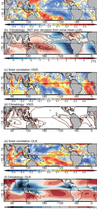
Therefore, the solar influence in the tropics is investigated for this season. Figure 11 shows correlation coefficients for boreal summer (JJA) between the solar index and (a) SSTs, (c) meridional wind velocity at 925 hPa and (e) outgo- ing longwave radiation (OLR). Summertime climatologies are also displayed below the respective correlation plots;

Fig. 11b depicts climatological SSTs (contours) and their deviation from the zonal mean SST (colour shading). The climatological northward component of the wind velocity at 925 hPa is displayed with 2 m s⁻¹contours (Fig. 11d). Figure 11e shows climatological OLR (colour shading). Regions of negative solar SST signals (Fig. 11a) roughly coincide with

0 0 0 0 0 0

0 0 0

0 0

0

0 0

0 0 0

0

0 0

60 120 180 −120 −60 0

−15015

−0.4 −0.3 −0.2 −0.1 0.0 0.1 0.2 0.3 0.4

(a) Solar correlation: SST

27 27

27

27 28

28 28

28

29 29

60 120 180 −120 −60 0

−15015

−4 −3 −2 −1 0 1 2 3 4 [^OC]

(b) Climatology: SST and deviation from zonal mean (JJA)

0 0

00 0 0

0 0 0

0

0 0 0

0 0

00 0 0 0

0

0 0

0

60 120 180 −120 −60 0

−15015

−0.4 −0.3 −0.2 −0.1 0.0 0.1 0.2 0.3 0.4

(c) Solar correlation: V925

2

2 2 2

2

2 2 2

2

2 2 2

2

2 4

4 4 4

4 4

4

4 4

6 6

60 120 180 −120 −60 0

−15015

(d) Climatology: V925

0 0 0 0

0 0

0 0 0

0

0 0 0

0

0 0 0 0

0

0 0 0 0

0

60 120 180 −120 −60 0

−15015

−0.4 −0.3 −0.2 −0.1 0.0 0.1 0.2 0.3 0.4

(e) Solar correlation: OLR

60 120 180 −120 −60 0

−15015

220 240 260 280 OLR [W m ]^-2

(f) Climatology: OLR

JJA mean

Figure 11.Boreal summer (JJA) solar signal in(a)SST,(c)meridional winds at 925 hPa and(e)OLR, presented as correlations with the solar index for the period 1979–2010.(b)JJA mean climatological SST, with contours for 27, 28 and 29^◦C, and colour shading denoting the deviation from the latitudinal mean SST.(d)Climato- logical JJA northward wind component at 925 hPa (contours every 2 m s⁻¹).(f)Climatological JJA OLR (colour shading).

regions of low climatological SST with respect to the zonal mean, such as in the southeastern Pacific, the South Atlantic and the coastal Arabian Sea. These sectors are also characterized by strong cross-equatorial winds along the conti-