Peak group analysis for the extraction of pure component spectra. Mathias Sawall

(1)

Peak group analysis for the extraction of pure component spectra.

Mathias Sawallâ, Christoph Kubis^b, Enrico Barsch^b, Detlef Selent^b, Armin Börner^b, Klaus Neymeyrâ,b

aUniversit¨at Rostock, Institut f¨ur Mathematik, Ulmenstrasse 69, 18057 Rostock, Germany

bLeibniz-Institut f¨ur Katalyse e.V. an der Universit¨at Rostock, Albert-Einstein-Strasse 29a, 18059 Rostock, Germany.

Abstract

Structure elucidation for the reactive or catalytic species of a chemical reaction system can significantly be supported by spectroscopic measurements. If the spectroscopic data contains isolated signals or groups of partially separated peaks, then the identification of correlations between these peaks can help to determine the pure components by their functional groups.

A computational method is presented which constructs from a certain frequency window, which contains a single peak or a peak group, an associated pure component spectrum on the full frequency range. This global spectrum reproduces the spectrum in the local frequency window or, at least, reproduces the contribution from the dominant component in the local window. The method is called the Peak Group Analysis (PGA). The methodological background of the PGA are a multivariate curve resolution method and the solution of a minimization problem with weighted soft constraints. The method is tested for two experimental FT-IR data sets from investigations into equilibria of hydroformylation catalysts based on rhodium and iridium. An implementation of the PGA is presented as a part of the FACPACK software.

Key words: factor analysis, pure component decomposition, nonnegative matrix factorization, spectral recovery.

1. Introduction

Spectroscopic methods in combination with chemometric techniques are key tools for the determination of unknown chemical species in a reaction system. Here we consider a situation in which the course of a chemical reaction is recorded spectroscopically. If a series of k spectra is taken and each spectrum is a vector of n absorbance values, then the spectral data can be stored row-wise in a k-times-n matrix D. The Lambert-Beer law in matrix form D=CA says that D can be factored in a product of two nonnegative matrices, namely in a concentration factor C and a spectral factor A. In the case of slightly perturbed, experimental data the aim is to determine at least an approximate factorization. If the reaction system contains a number of s independent components, then C ∈ R^k×s contains columnwise the concentration profiles in time of the s pure components.

The spectral factor A∈R^s×ncontains row-wise the pure component spectra. Such a factorization of D has first been conducted for a two-component system by Lawton and Sylvestre [1]. A fundamental problem of such factorizations is that the matrix factors are not unique due to the so-called rotational ambiguity [2, 3].

The four volumes of the book series Comprehensive

Chemometrics [4] give a detailed overview on the wide range of chemometric methods and its mathematical analysis. Without claiming any completeness we would like to mention the evolving factor analysis [5], the window factor analysis [6], which each can be combined with Manne’s theorems [7], as well as the target factor analysis [8] and, last but not least, the class of Multi- variate Curve Resolution (MCR) methods with hard and soft constraints [9, 10].

1.1. The idea underlying the peak group analysis In the present paper our objective is a bit different.

We do not directly seek to compute a nonnegative fac- torization D = CA, but we try to extract single spec- tra and to identify related peak groups in order to determine some of the species by their functional groups.

Our approach is driven by practical needs of the chemist who has some presumptions and assumptions on the species which might be found in the chemical reaction system. For instance in organo-metallic/catalytic chem- istry the (IR-)spectra of the reactants and the spectra of the main reaction products are known, but the catalytic active species and the catalyst preformation process is sometimes unknown [11]. However, reasonable

July 30, 2015

(2)

assumptions on the catalytic active species can be made.

Together with the molecular point group of the catalyst or its precursor, the character table provides insight into active and characteristic vibrations. Alternatively one can compute reliable approximations of the absorption spectrum by quantum mechanical SCF computations or DFT calculations. For these reasons that the chemist, after having identified a certain signal (like stretching vibrations of terminal carbonyl ligands in rhodium carbonyl complexes), would like to know if this signal is part of a pure component spectrum which also includes a characteristic signal that is associated with a further functional group [12, 13]. In this paper we present a numerical algorithm, called Peak Group Analysis (PGA), which aims at finding correlations between peaks and peak groups which are associated with the same pure component. Mathematically, the algorithm uses a spe- cific target function which includes a weighted combination of soft constraints. The approach is based on a local rank-one reconstruction; its application to spectroscopic data with narrow and partially isolated peaks, which can typically be found in IR spectroscopic data, works very well.

1.2. Overview

In Section 2 a short introduction to the basics of multivariate curve resolution techniques is given and the idea of the PGA is explained. Section 3 presents the mathematical foundation of the PGA and its target function. Further the soft constraint functions are introduced. Some mathematical theorems on the construction of the concentration profiles are contained in Sec- tion 4. Section 6 refers to the FACPACK implementation of the PGA [14, 15]. Finally, the application of the PGA to experimental FT-IR data sets is discussed in Section 8.

2. Peak group analysis (PGA) 2.1. Aim of the PGA

The aim of the PGA is to identify those peaks or peak groups in a series of spectra taken from a chemical mixture which can be assigned to the same pure component. The starting point is the specification of a frequency window which contains a certain peak or peak group. Then the PGA intends to provide a pure component spectrum which in the given frequency window more or less reproduces the original signal. The PGA can be applied repeatedly in order to find all pure component spectra step-by-step.

2.2. The general MCR approach

The general approach to reconstruct the pure com- ponent factors C and A is based on the singular value decomposition (SVD) of D [1]. Let U ∈R^k×k,Σ∈R^k×n and V ∈ R^n×n be the factors of the SVD, so that D = UΣV^T [16]. Furthermore let s be the number of inde- pendent components underlying the data D; for noise- free data the number s equals the rank of D. Then C and A can be reconstructed only by using the first s left- and right singular vectors [6, 8].

In the case of noisy data it is often advantageous to work with a number of z ≥ s singular vectors for the reconstruction of C and A [10]. Then the mathematical formulation reads

C=UΣT⁺, A=T V^T (1)

with U, Σ and V^T containing the first z singular vec- tors and singular values. The associated transformation T ∈R^s×zis a rectangular matrix. Further T⁺ ∈R^z×sis the so-called Moore-Penrose pseudoinverse of T . This SVD based reconstruction approach reduces the number of degrees of freedom of the factorization problem to sz which is the number of matrix elements of T . Finally, the determination of feasible and chemically meaning- ful matrix factors C and A amounts to the computation of a proper matrix T ∈R^s×z.

2.3. Construction of a single pure component spectrum Equation (1) is a construction for the simultaneous formation of the spectra and concentration profiles for all factors. In contrast to this the PGA determines the pure component spectra, which are the rows of A, step- by-step. Mathematically a pure component spectrum a ∈ R^1×n is a linear combination of the z right singu- lar vectors which belong to the z largest singular vec- tors. The spectra are written as row vectors so that a has the form a = t V(:,1 : z)^T. Our task is to de- termine the vector t ∈ R^1×z of expansion coefficients.

These z degrees of freedom can be reduced to z −1 since any nonzero scaling of the spectrum is without relevance. The Perron-Frobenius theory on the spectrum of a nonnegative matrix [17] provides under mild assumptions on the spectral data matrix D, see Theo- rem 2.2 in [15], that the first coefficient t1is never equal to zero. The mathematical argumentation is as follows:

the Perron-Frobenius theory guarantees that V(:,1) is a sign-constant vector. Without loss of generality it can be assumed as a component-wise nonnegative vector. Or- thogonality of this vector to any linear combination of the remaining singular vectors V(:,2), . . . ,V(:,n) proves 2

(3)

that this linear combination must have positive and neg- ative components. Since a feasible spectrum must have only nonnegative components, any feasible spectrum must have a contribution from V(:,1).

All this justifies to use a scaling so that t₁=1, which for instance has been used in [18, 19, 14] and for the re- solving factor analysis (RFA) [8]. Thus t can be written in the form t = t1(1,w) with w ∈ R^1×z−1 and t1 > 0.

Thus we get a=t1(1,w)V^T.

2.4. Window selection and normalization

The starting point of the PGA is the selection of a channel window [ν_ℓ, ν_r] along the wavenumber/frequency axis. This window should contain a single peak or group of peaks whose affiliation to other peaks or peak groups of the same pure component within the series of spectra is to be analyzed. The channel window [νℓ, νr] contains the discrete wavenumber values νi with respect to the given grid. The set I⊂ {1, . . . ,n}is the maximal set of indices so that

νℓ ≤νi≤νr, for all i∈I.

For the following construction of a pure component spectrum a, which reproduces more or less the selected signal in the window [νℓ, νr], it is useful to normalize a∈Rⁿin I in a way that

maxi∈I ai=1. (2)

Together with the non-normalized representation a = t1(1,w)V^Tand ai=t1(1,w)V(i,:)^Twe prefer to work in the following with the normalized form

a=a[w] := (1,w) V^T

maxi∈I((1,w) V(i,:)^T). (3) 2.5. Stepwise extraction of the pure component spectra The PGA can be applied repeatedly to a given series of spectra. In each cycle the spectrum of a single component can be extracted. The method works very well especially for IR spectroscopic data with its typically narrow and isolated peaks, see Section 8. If for a cer- tain component the spectrum a (row vector) has been extracted and if for this component the concentration profile c (column vector) is accessible, then the contri- bution of this component to the spectral data matrix D can be removed by subtracting a proper multiple of the rank-1-matrix ca∈R^k×nfrom D. The principles of such a rank-1-downdate of a nonnegative matrix in order to construct in the end a complete nonnegative matrix factorization has been analyzed in [20]. In every step the

contribution of one component is removed from D and finally and ideally only the noise remains. The expla- nation is simple, but in practice such an approach has severe disadvantages due to the influence of noise. The decisive point is that such a stepwise rank-1-downdate of D is very sensible with respect to noise, since the errors of all previous rank-1-downdates accumulate in D. For instance the subtraction of a rank-1-matrix may result in small negative components in D or the subtrac- tion of a certain peak of a slightly perturbed amplitude or frequency position could result in a small remaining peak with a somewhat shifted frequency position.

All this adversely affects the accuracy of the subsequent rank-1-downdates.

Alternatively one can always work with the original spectral data matrix D without subtracting rank-1 ma- trices [21]. This reduces the impact of noise. If finally a series of s independent pure component spectra has been determined, then the associated concentration fac- tor C can be computed by a “global” least-squares com- putation. Such a procedure appears to be more stable.

2.6. Application to IR data

By construction the PGA can be applied to spectral data which contains several narrow peaks and which also includes, at least for some time intervals, frequency ranges in which no absorption is observed. If, contrary to the foregoing, all pure component spectra show an absorption on the whole frequency range, then it would be difficult for the PGA to extract the contribution from a single component.

In particular the IR or Raman spectroscopy provide data with narrow peaks and several non-absorbing frequency ranges. Then a step-by-step extraction approach could successfully be applied; this has clearly been demonstrated by the BTEM software by Garland and his group [21]. A further technique which is based on a local analysis is SIMPLISMA [22, 23] which has been successfully applied to IR spectral data. In contrast to this the UV/Vis spectroscopy results in spectra which are rather unsuitable for an application of the PGA. Fi- nally, the PGA can principally be applied to NMR data [24]; however the occurrence of the nuclear magnetic resonance chemical shifts necessitates a proper data pre- processing.

2.7. Relations to EFA, WFA and TFA techniques The evolving factor analysis (EFA) [5] and the window factor analysis (WFA) [6] are powerful techniques for the analysis of spectroscopic data. EFA analyzes 3

(4)

the evolution of the rank of a series of growing sub- matrices of D. WFA computes the concentration pro- file of a certain component by using submatrices along the time axis for an evolutionary process; together with Manne’s theorem pure component information can be extracted. There are some similarities between the WFA and the PGA, but there are also two differences. First, PGA uses windows along the frequency axis. Second, WFA and EFA are rather fixed computational procedures, whereas the PGA is based on an optimization process with a target function which includes several regularization terms, see Section 3.

Finally, the PGA is very different from the target factor analysis (TFA) [8] where a given factor (spectrum) is tested, whether it contributes to the spectral measure- ment or not. For the PGA no spectrum has to be known initially.

3. The target function for the PGA

Equation (3) shows the way how to compute a single pure component spectrum a by means of a row vector w ∈ R^z−1. Next w is determined by the solution of a minimization problem for a target function which includes several weighted constraints. The choice of the constraint functions and their weight factors is a crucial step. Their suitable selection depends on the type of the spectroscopic data. The solution of constrained minimization problems for the computation of nonnegative matrix factorizations is a standard procedure in chemometrics, see e.g. [25, 26, 27, 21, 9, 2, 28, 10].

The PGA target function f is formed by a weighted mean of two functions f1and f2which is combined with several weighted soft constraints

f (w)=ω1f1(a[w])+ω2f2(a[w])+ Xq

i=1

γ²_igi(a[w]) (4) with a[w] by (3); in the following we simply write a for a[w]. Thereinωi≥0 andγi≥0 are the weight factors.

The functions f1and f2are:

1. Norm of the spectrum:

f1= Xn

j=1

a²_j.

A spectrum with a small integral and narrow peaks is favored.

2. Norm of the discrete second derivative of the spectrum:

f2= Xn−1

j=2

aj−1−2aj+aj+1

(∆ν)²

!2

with ∆ν being the wavenumber increment along the equidistant wavenumber grid. The function f2

is the sum of squares of the discrete second deriva- tive of the spectrum a with respect to equidistant grid of wavenumber values. By f2 a smooth spectrum is favored.

The constraint functions are introduced in Section 3.1.

3.1. Constraint functions

The construction of the soft constraints, also called regularization functions, and their weighting is decisive for the computation of meaningful pure component spectra. In order to construct a flexible curve resolution method, which can be applied to several series of spectra from different types of spectroscopic techniques with their different typical shapes, it is useful to have a stock of various regularization functions, see [21, 9, 10]

for diverse examples.

For the PGA the following soft constraints are available (and can or cannot be used depending on the present conditions that, e.g., certain spectra are known or are not known):

- Nonnegativity.

- Local reconstruction error,

- Distance (by the sum of squares) to a given pure component spectrum. This constraint is similar to the target factor analysis [8],

- Correlation with other pure component spectra.

All these constraint functions have been written in a functional form depending on a. By (3) a depends on w so that these functions essentially depend on the z−1 components of w.

Within each step of the optimization the current ap- proximation of a spectrum a can be used in order to compute a temporary concentration profile c with re- spect to the channel window I according to

c=UΣυ^∗ with υ^∗=V(I,:)^Ta(I)^T

ka(I)k²₂ . (5) The resulting pair a and c allows an optimal reconstruc- tion of D in the channel window I; see Section 4 for the mathematical analysis. It is important to note that c and a are only temporary approximations which are changed within each step of the optimization procedure. A fur- ther important point is that a ≥0 and D≥0 imply that 4

(5)

c≥0; a proof of this fact is given in Corollary 4.2. The result that c ≥0 shows that no further constraint func- tion has to be added to f in order to guarantee the non- negativity of c. At the end of the iterative minimization, Equation (5) can also be used to compute from the final spectrum a a final approximation of the concentration profile c.

The constraint functions g_i : Rⁿ → R+read as follows:

1. Nonnegativity: The constraint function which is used to favor an almost nonnegative solution a is

g1= Xn

j=1

min aj

kak∞

+ε,0

!2

.

Thereink · k∞ denotes the maximum norm which is maximum of the absolute values of the components. A small value ε ≥ 0 is used to al- low slightly negative components for which the ra- tio min aj/kak∞ is larger than−ε; accepting such small negative entries can be very helpful for finding a solution in the case of noisy data. In Corol- lary 4.2 it is shown that the associated concentra- tion profile c is nonnegative, if a and D are non- negative. Hence a constraint function on the non- negativity of c is not needed.

2. Local reconstruction: Withυ^∗by (5) and c=UΣυ^∗ the local reconstruction error is

g2= Σ



V(I,:)^T−V(I,:)^Ta(I)^Ta(I) ka(I)k²₂





2

F

.

Therein a(I) and V(I,:) are the vector resp. matrix which are reduced to the indices contained in the index set I. Furtherk · kF is the Frobenius norm, which is the square root of the sum of squares of its argument.

3. Distance to a given spectrum ˆa∈R^1×n: This constraint function measures the distance of the opti- mally scaled ˆa to a

g3 = Xn

j=1

(αâj−aj)² with α= âa^T kâk²₂

=kak²− ˆaa^T kˆak².

4. Correlation with other spectra: This constraint function favors a solution with a small correla- tion with other pure component spectra A(i,:), i=

1, . . . ,s0,

g4=

s₀

X

i=1

Xn

j=1

(A(i,j) aj)².

3.2. Numerical solution of the minimization problem The target function f in (4) defines a nonlinear least squares problem with z−1 free variables. In our FAC- PACK implementation of the PGA, see Section 6 we use a combination of genetic algorithm and of the ACM software NL2SOL [29] written in FORTRAN.

A careful choice of the weight parameters, especially the choice ofω1andω2, is very important for computing reliable and meaningful spectra. If a channel window is selected which contains peaks originating from more than one component, then the local reconstruction cannot be successful andγ2should be relatively small.

4. Concentration profiles by local reconstruction A well-known approach to construct the concentra- tion profile c which fits bests to a certain pure compo- nent spectrum a is to compute

c=Da⁺

with the pseudo-inverse a⁺of a, see e.g. Equation (5) of [21]. With the representation a=tV^T of a it holds that

c=Da⁺=UΣV^TVt⁺=UΣt⁺. The pseudo-inverse of t reads

t⁺= t^T

ktk²₂ = V^Ta^T

kaVk²₂ = V^Ta^T kak²₂

so that

c=UΣυ withυ=V^Ta^T

kak²₂ . (6) This representation of c is similar to the “windowed”

representation by Equation (5) which has the form c=UΣυ^∗ withυ^∗= V(I,:)^Ta(I)^T

ka(I)k²₂ . (7) In this section a proof is given that the windowed representation (7) is a suitable generalization of (6) which has optimal reconstruction properties with respect to the channel window I.

The central ideas for the reconstruction of c are as follows: A single spectrum a ∈ R^1×n should be asso- ciated with a single concentration profile c ∈ R^k×1 so 5

(6)

that the rank-1 matrix ca is a best approximation of the spectral data D within the channel window which is de- termined by the index set I. The restriction D|_I of D to the channel window I is given by

D_I =UΣV(I,:)^T and the rank-1 matrix ca with a=tV^Treads

ca= UΣυ

|{z}

c

tV^T

|{z}

a

.

The restriction of ca to the channel window I is ca_I =UΣυtV(I,:)^T.

Under the assumption that the spectral signal in the channel window I is determined only by a single com- ponent, the difference function

f (υ)=D_I−ca_I²_F =UΣV(I,:)^T−UΣυtV(I,:)^T²_F is to be minimized.

In Theorem 4.1 and in Corollary 4.2 a minimizerυ^∗ is determined. It is shown that the concentration profile c = UΣυ^∗is nonnegative if a and D(:,I) are nonneg- ative. Finally, Lemma 4.3 presents an error estimation for C(:,i)−c.

Theorem 4.1. Let D∈R^k×nwith rank(D)≥z be given and let U∈R^k×z,Σ∈R^z×zand V∈R^n×zbe the factors of a truncated singular value decomposition of D. Fur- thermore let I⊂ {1, . . . ,n}be the index set of the chan- nel window. The vector t ∈R^1×zdetermines a nonzero spectrum a=tV^T and it is assumed that the restriction of a to I, which is denoted by a_I =: a(I) does not vanish, i.e.ka(I)k>0.

Then the local reconstruction error

f (υ)=UΣV(I,:)^T−UΣυtV(I,:)^T²_F (8) attains its minimum inυ^∗∈R^1×zwith

υ^∗=V(I,:)^TV(I,:) t^T

kV(I,:) t^Tk²₂ =V(I,:)^Ta(I)^T

ka(I)k²₂ . (9) With the associated optimal concentration profile c= UΣυ^∗ the rank-1 reconstruction ca results in a rank-1 downgrade of D

rank(D−ca)=rank(D)−1. (10)

Proof. Due to the orthogonal invariance of the Frobenius-norm [16] the distance f (υ) can be simplified

f (υ)=ΣV(I,:)^T−ΣυtV(I,:)^T²_F

= Xz

j=1

X

i∈I

σ²_jV_{i j}²−2 Xz

j=1

σ²_jυj

X

i∈I

Vi j

Xz

l=1

tlVil

+ Xz

j=1

σ²_jυ²_jX

i∈I





Xz

l=1

t_lV_il





2

.

The gradient vector has the form

∇f (υ)=0−2Σ²V(I,:)^TV(I,:) t^T+2kV(I,:) t^Tk²₂Σ²υ and ∇f (υ^∗) = 0 as a necessary condition for an ex- tremum results in (7). The Hessian of f (υ) reads

Hf(υ)=2kV(I,:) t^Tk2Σ²=2ka(I)k2Σ². Since rank(D) ≥z the truncated matrixΣhas the maximal rank and together with ka(I)k > 0 the Hessian Hf(υ^∗) is a positive definite matrix. Hence f attains its minimum inυ^∗.

In order to prove (10) we need the following relation for the n×n identity matrix I and column vectors a,b∈ Rⁿ: The matrix I−ab^Tis regular if and only if a^Tb,1.

This relation follows from the more general Sherman- Morrison-Woodbury formula [16]. For the given special case the proof is simple. If I−ab^T is regular, then (I− ab^T)a = a−a(b^Ta) , 0 only if b^Ta , 1. To prove the other direction one has to check that the inverse of I−ab^Tis (I+ab^T/(1−b^a)).

For t andυ^∗it holds that

tυ^∗= t V(I,:)^TV(I,:) t^T kV(I,:) t^Tk²₂ =1 so that

D−ca=D−UΣυ^∗tV^T =UΣ(I−υ^∗t)V^T. Since I−υ^∗t is a singular matrix with the rank z−1 the same holds for D−ca.

The concentration profile c by Theorem 4.1 is non- negative if D and a are nonnegative. This is proved next.

Corollary 4.2. Let the assumptions of Theorem 4.1 be satisfied and let D(:,I)≥0 as well as a=tV^T ≥0.

Then the associated concentration c =UΣυ^∗is also nonnegative.

6

(7)

Proof. Since D(:,I)≥0 and a(I)≥0, it holds that c=UΣυ^∗=UΣV^T(I,:) a(I)

ka(I)k²₂ = D(:,I) a(I)^T ka(I)k²₂ ≥0.

(11)

The factors a and c arise by construction from a local factorization within the channel window I. If D=CA is the correct global factorization of D, then a and c should be (aside from scaling) recoverable as a certain row of A and as the associated column of C so that a =A(i,:) and c=C(:,i) for a suitable index i.

The difference between c (by the local construction) and the associated column C(:,i) (as determined by the global factorization) depends on the computed a and on the absorption by the other species in the window I. An error-estimation for c−C(:,i) is given in the following lemma.

Lemma 4.3. Let the assumptions of Theorem 4.1 be sat- isfied, let m be the number of channel indices in I and let a(I) = tV(I,:)^T and c as given in (7). Further let D=CA be a feasible nonnegative factorization so that a equals A(1,:) on the interval I, which is a(I)=A(1,I).

Finally let

E = Xs

i=2

C(:,i)A(i,I)

be the sum of all absorptions by all other components in the channel window I.

Then the errorkc−C(:,1)k2 is bounded from above as

kc−C(:,1)k₂≤ kEk2

kA(1,:)k2

.

ThereinkEk2 =maxa,0kEak2/kak2is the spectral oper- ator norm.

Proof. With c=D(:,I) a(I)^T/ka(I)k²₂by (11) and a(I)= A(1 :,I) it holds that

c=





Xs

i=1

C(:,i) A(i,I)



 a(I)^T ka(I)k²₂

=C(:,1)+E a(I)^T ka(I)k²₂.

With respect to the Euclidean norm and the associated spectral norm one gets

kc−C(:,1)k₂= kE a(I)^Tk2

ka(I)k²₂ ≤ kEk2

ka(I)k2

. (12)

A useful consequence of (12) is the following: If the inner products of a with all other pure component spectra within the window I are equal to zero, then c =C(:,1) and the pure component concentration profile is reproduced exactly.

In Remark 4.4 an estimate for the error c−C(:,1) for the case that c is constructed by the non-windowed pseudo-inverse of t in the form c=UΣt⁺. According to our experience the windowed reconstruction of c by 4.1 provides the better results for the concentration profiles compared to the construction with the pseudo-inverse of t. The different approaches are compared in Section 8.2 for experimental data.

Remark 4.4. Let the assumptions of Lemma 4.3 be sat- isfied. If the concentration profile c is computed by c =UΣt⁺with the pseudo-inverse t⁺of t and A(1,:) = a=tV^T, then the error vector c−C(:,1) reads

c−C(:,1)= 1 kA(1,:)k²₂

Xs

i=2

C(:,i)A(i,:)A(1,:)^T. (13) Its Euclidean norm is bounded from below and above in the form

α≤ kc−C(:,1)k2≤β with

α=maxi=2,...,skC(:,i)k2A(i,:)A(1,:)^T

kA(1,:)k² , (14) β=

Ps

i=2kC(:,i)k₂A(i,:)A(1,:)^T

kA(1,:)k² . (15) Proof. With a=A(1,:)=tV^T and a⁺=(tV^T)^T/ktV^Tk²₂ it holds that

c=UΣt⁺=UΣt^T/ktk²₂ =UΣV^TVt^T/ktV^Tk²₂

=D(tV^T)⁺=Da⁺=DA(1,:)⁺

=





Xs

i=1

C(:,i)A(i,:)



A(1,:)⁺

=C(:,1)+





Xs

i=2

C(:,i)A(i,:)



A(1,:)⁺.

This together with A(1,:)⁺ =A(1,:)^T/kA(1,:)k²₂results in (13). The bounds (14) and (15) can easily be proved.

The difference (13) vanishes if and only if A(i,:)A(1,: )^T = 0 for all spectra i = 2, . . . ,s. This condition is more restrictive compared to (12) where only a local condition with respect to the channel window I has to hold. Thus the error for c−C(:,1) is expected to be larger compared to the estimate from Lemma 4.3.

7

(8)

5. Delimitation to alternative MCR methods The PGA method is one among many alternative and well-established MCR methods. Explicitly we would like to mention the famous MCR-ALS toolbox [9], the resolving factor analysis (RFA) [30], the SIMPLISMA algorithm [22], the band target entropy minimization (BTEM) [21] and the pure component decomposition (PCD) [10].

All these methods focus on the computation of a sin- gle nonnegative factorization D = CA. However, due to the rotational ambiguity there are nearly always con- tinua of nonnegative factorizations which can be computed by global MCR-methods and which can be rep- resented by the so-called Area of Feasible Solutions (AFS). Computationally the AFS can be determined, e.g., by the FACPACK software [31, 32]. The strategy of the first-mentioned MCR methods is to filter out only a single factorization by means of soft constraints. A reliable MCR method should provide a good approximation of the chemically correct solution. The general approach of all these MCR-methods is to construct a cost function which depends on the transformation ma- trix T , see (1), and whose feasible matrix elements are associated with the AFS. However, the minimization of the soft-constrained cost function results in the desired matrix factors C and A. With this approach the com- puted solution strongly depends on the choice of the constraints. The numerical computation of the global minimum of the cost function is sometimes a difficult numerical problem as the numerical minimization may get stuck a local minimum.

5.1. Benefits of the PGA algorithm

A characteristic trait of the PGA algorithm is that the pure component spectra are computed step-by-step, whereas other methods like RFA or PCD compute all spectra (and concentration profiles) simultaneously. Ac- cording to our experience, PGA is a robust algorithm for medium-to-strong perturbed spectral data. The method also works very well in case of systematic perturbations for example from a suboptimal baseline correc- tion. Whenever MCR methods like RFA, MCR-ALS or PCD show difficulties in the simultaneous computation of the spectra and concentration profiles, the PGA algorithm can be applied in order to try a stepwise decomposition. Then PGA may extract single pure components and can be able to uncover correlations within highly overlapping peak groups. The technical reason for these abilities are the window analysis of the spectra and the reduced number of variables of the cost function.

The strategy underlying the PGA method shows some resemblance to the BTEM algorithm [21]. BTEM also allows a step-by-step extraction of the pure component spectra. However, the computational procedures of PGA and BTEM are different. Compared to BTEM the number of unknown variables is reduced from z to z−1. Further, PGA works with a different construction of the associated concentration profile by using a windowed pseudo-inverse construction. In BTEM the pseudo-inverse is used for a global fit, whereas for PGA the potentially more stable local approximation from (5) is applied. See Lemma 4.3 and Remark 4.4.

5.2. Limitations of a step-by-step factorization

The higher robustness of PGA with respect to noise by means of a windowed step-by-step decomposition has to be paid with a partial loss of insight to the global correlations between the factors. In other words, step-by-step computed concentration profiles and spec- tra must not necessarily result in factors C and A with a small reconstruction error D−CA. Whenever the data does not include systematic perturbations or a consider- able portion of noise one should first apply MCR methods like RFA, MCR-ALS or PCD.

6. PGA and the FACPACK software

The FACPACK software is a program package for the computation of multi-component factorizations and the area of feasible solutions for two- and three-component systems by means of the polygon inflation method [14, 15]. This software also allows the simultaneous representation of C and A and a step-by-step construc- tion of the pure component factors by using arguments from the complementarity theory [31].

The peak group analysis (PGA) is a separate module of the forthcoming revision 1.2 of FACPACK, which is planned to be published in the second half of the year 2015. The current revision of the software can be down- loaded from the web page

http://www.math.uni-rostock.de/facpack/

7. Analysis of a model problem

Next the PGA method is applied to a three- component model problem with a number of k = 201 spectra each with n = 501 channels. The simulated concentration profiles, the columns of C, and the pure component spectra, the rows of A, are shown in Figure 8

(9)

0 0.5 1 1.5 2 0

0.2 0.4 0.6 0.8 1

Concentration profiles

10 100

0 0.2 0.4 0.6 0.8 1

Pure component spectra

Figure 1: The concentration profiles, the columns of C, are shown together with the pure component spectra, the rows of A, for the model problem from Section 7. In a second step noise is added to the product D=CA.

20 40 60 80 100

0 0.2 0.4 0.6 0.8 1

Case of weakly overlapping peaks

20 40 60 80 100

0 0.2 0.4 0.6 0.8 1

Case of strongly overlapping peaks

Figure 2: Window selection in the series of spectra with normal distributed noise. Left: Three windows positioned on the well-separated peaks, Right: Three windows positioned on the three strongly overlapping peaks.

1. The spectral data matrix is D = CA. Noise of dif- ferent types, namely random noise and systematic noise or bias, are added to the data in order to demonstrate the capabilities of the PGA method. The perturbed data sets are shown in Figure 2 (case of random noise) and in the left subplot of Figure 5 (systematic noise). More information is given below.

7.1. Overlapping peaks

The pure component spectra are constructed in a way that each spectrum contains three peaks and each peak is a Gaussian. One peak for each spectrum is relatively isolated; these peaks are centered at x0 =25, x0 = 30 and x0 =35. A second peak of each spectrum strongly overlaps with one peak of the other pure component spectra; the three peaks are centered at x0 =50, x0=53 and x0 = 56. A third peak of each spectrum is cen- tered at x0 = 80 and has the amplitude 1. Thus this peak completely overlaps with the other spectra. How- ever, the three peak widths are slightly different. See the right subplot of Figure 1 for these three spectra.

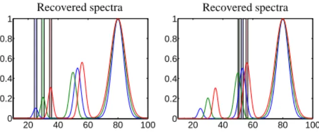
7.2. PGA applied to windows on well-separated peaks First PGA is applied to the data matrix D plus ran- dom noise (normal distributed noise with a standard

20 40 60 80 100

0 0.2 0.4 0.6 0.8 1

Recovered spectra

20 40 60 80 100

0 0.2 0.4 0.6 0.8 1

Recovered spectra

Figure 3: PGA results on the pure component spectra for data including random normal distributed noise. Left: Recovered pure component spectra for the case of isolated peaks, see left subplot in Figure 2. Right: Recovered pure component spectra for the case of strongly overlapping peaks, see right subplot in Figure 2. The original pure component spectra are plotted in black lines.

deviation of 0.002 and mean 0). As the model problem includes three independent components, three separate windows are selected for the calculation of the three pure component spectra. First, small windows are placed at the three isolated peaks at x0 =25, x0 =30 and x0=35. These three narrow windows in gray color are shown in the left subplot of Figure 2. These windows are the basis for the identification of the associated pure component spectra.

The weights factorsωi andγi, see Equation (4), are set toω1 =0.1,γ1=10,γ2 =1.5 andω2 =γ3 =γ4 = 0. The reconstruction is based on a number of z = 3 singular vectors. The computed pure component spectra are shown in Figure 3. The relative reconstruction error

ei= kA^(orig)(i,:)−a^(PGA)(i,:)k2

kA^(orig)(i,:)k2

, i=1,2,3, (16) allows to compare the results with the original solutions.

We get e=(4.7·10⁻³,1.5·10⁻²,1.1·10⁻²). Thus PGA works very well.

7.3. PGA for strongly overlapping peaks

Next we demonstrate the capability of the PGA to identify peak correlations and peak groups for the case of overlapping peaks. Therefore the three windows are placed around the three centers x0 = 50, x0 = 53 and x0 = 56 which belong to strongly overlapping peaks.

Once again the three pure component spectra are reconstructed from the noisy data, see Section 7.2 on the noise intensity. The window selection is plotted by gray bars in the right subplot of Figure 2.

For the PGA we used the weight factorsω1 = 0.1, γ₁ =10,γ₂ =0.5 andω₂ =γ₃ =γ₄ =0. The number of singular vectors is z=3. The solutions are presented in the right subplot of Figure 3. Even for these strongly overlapping signals PGA works very well and the correct single pure component spectra have been identified 9

(10)

1 2 3 4 5 6 7 8 10⁻¹⁰

10⁻⁵ 10⁰

Singular values of D

i σi noisy data

original data

Figure 4: The singular values of the data matrix D including system- atic noise (×) and the singular values of the non-perturbed data (◦).

The non relatively large singular valuesσ4,σ5,σ6are a clear indica- tor of the presence of systematic noise (bias).

with errors less than one percent. The error vector (16) reads e=(3.7·10⁻³,7.9·10⁻³,6.8·10⁻³).

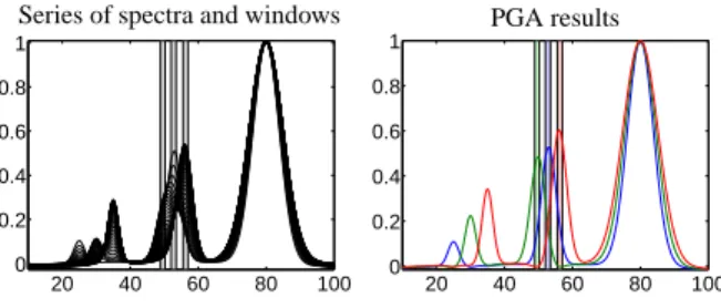
7.4. PGA and systematic noise

Next PGA is applied to the data including systematic noise. Therefore D is computed as

Di,j= X3

ℓ=1

Ci,ℓAℓ,j+0.005



2−(x_j−50−₁₀ⁱ)² 500



 (17) for i = 1, . . . ,201 and j = 1, . . . ,501. The series of spectra including these perturbations is shown in the left subplot of Figure 5. The first eight singular values of the data matrix D are shown in Figure 4. Due to the perturbation, see (17), the singular valuesσ4,σ5andσ6

are very different from the non-perturbed data. For non- perturbed data the matrix has the rank 3. Hence these singular values are equal to zero aside from rounding errors.

For the PGA computation the windows are located on the strongly overlapping peaks. A number of z = 4 singular vectors is used. The selected windows and the computed pure component spectra are presented in Figure 5.

Even in presence of systematic noise (bias) and for the strongly overlapping peaks it is possible to identify the correct pure component spectra with the PGA. The error vector reads e=(2.8·10⁻²,3.7·10⁻²,5.1·10⁻²).

8. Application to IR data from experimental stud- ies of equilibria of rhodium and iridium hydro- formylation catalysts

In this section the PGA is applied to FT-IR spectroscopic data on the formation of rhodium-carbonyl

20 40 60 80 100

0 0.2 0.4 0.6 0.8 1

Series of spectra and windows

20 40 60 80 100

0 0.2 0.4 0.6 0.8 1

PGA results

Figure 5: Left: The three PGA windows positioned on the strongly overlapping peaks. Right: The PGA results of the pure component spectra. Even in presence of systematic noise PGA can correctly identify the pure component spectra.

clusters and on the catalyst formation for the iridium- catalyzed hydroformylation; see [33, 10, 12] for experimental details. Further an application of the PGA to weak signals is presented in Section 8.4. In this section the frequency axis for all spectra is given in wavenum- bers.

8.1. Rhodium-carbonyl complex formation from Rh(acac)(CO)₂

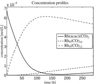
The displacement of the organic ligand acetylaceto- nate in Rh(acac)(CO)₂by CO is an unwanted side reaction in the formation of a catalytically active rhodium- hydridocarbonyl complex. In this experiment at 303 K and 20 bar synthesis gas pressure (CO:H2=1:1) the initial concentration of Rh(acac)(CO)₂is 6.6·10⁻⁴mol L⁻¹ in the solvent cyclohexane. Under these conditions the

”unwanted” rhodium carbonyl clusters Rh4(CO)₁₂ and Rh6(CO)₁₆together with Rh(acac)(CO)₂ are the dominating absorbing components. The spectrum of the solvent cyclohexane has been subtracted from the FT-IR spectroscopic data. A number of k = 292 spectra has been taken; each spectrum has n = 1479 channels. A subset of the series of spectra is shown in Figure 6.

In order to compute the pure component spectra of this system with s = 3 dominating components we have selected three separate channel windows for the application of the PGA. Each of these three windows [2005.5,2020.1]cm⁻¹, [1875.1,1893.9]cm⁻¹and [1812.7,1823.4] cm⁻¹contains only a single peak. The PGA has been applied three times with z = 4 and the weightsω1 =0.15 (first run to determine the first component), ω1 = 0.3 (second run to determine the second component) andω1 =0.15 (third run for the third component). Furtherω₂ = 0 in all program runs. In all these case f₁ and f₂ according to Equation (4) have been used. Further, only the constraint function g₁ and g2have been used with the weight factorsγ1 =10 and γ2 =1. This parameter selection has been used for all 10

(11)

1800 1900

2000 2100

0 100 200 0 0.1 0.2 0.3

wavenumber [1/cm]

time [h]

absorption

Figure 6: A subset of the k = 292 spectra for the formation of rhodium-carbonyl complexes from Rh(acac)(CO)2.

50 100 150 200 250

0 1 2 3 4 5 6 7x 10⁻⁴

time [h]

Concentration profiles

concentration[mol/L]

Rh(acac)(CO)₂ Rh6(CO)₁₆ Rh4(CO)12

Figure 8: The concentration profiles (absolute values) for the s=3 components by a global least-squares fit.

three PGA computations. The results, namely the pure component spectra of Rh(acac)(CO)₂, Rh4(CO)₁₂ and Rh6(CO)₁₆are shown in Figure 7.

The concentration profiles of these three components can be computed by the techniques introduced in Sec- tion 4; the use of Equation (9) is recommended. How- ever, in the present situation the three spectra of the three-component system are known. Hence it is more stable to form the matrix A and then to solve a global least-squares problem on the full wavenumber interval in order to compute C. Thus all three concentration pro- files are computed simultaneously. These profiles are shown in Figure 8.

8.2. Comparison of the different approaches to the computation of C

The most common way to compute a concentration profile which is associated with a single pure compo- nent spectrum a is to use the pseudo-inverse a⁺so that c=Da⁺or C(:,i)=UΣt⁺if the ith concentration pro- file is considered. The benefit of computing C(:,i) via υ^∗according to Theorem 4.1 is explained in Section 4.

Next C(:,i) is computed for the data set from Section 8.1 in three different ways:

1. Column-wise computation of C(:,i) = UΣυ(i)^∗ withυ(i)^∗by (9) for i=1,2,3.

2. Column-wise computation of C(:,i) = UΣt(i)⁺ with the pseudo-inverses t(i)⁺for i=1,2,3.

3. By a global (simultaneous) least squares fit in order to find C for known three pure component spectra given row-wise in A.

Figure 9 shows the results. The results for the approaches 1. and 3. are very similar, whereas the difference between the second and the third approach is only small for Rh(acac)(CO)₂. With respect to the Euclidean vector norm the distances

εi=C(:,i)−C^(global)₂/C^(global)₂, i=1,2,3, εi= eC(:,i)−C^(global)₂/C^(global)₂, i=1,2,3 with C=UΣυ^∗andCe=UΣt⁺are as follows

ε=(0.0034,0.0908, 0.0080), ε=(0.0856,4.5919, 0.0812).

8.3. Equilibrium of iridium complexes

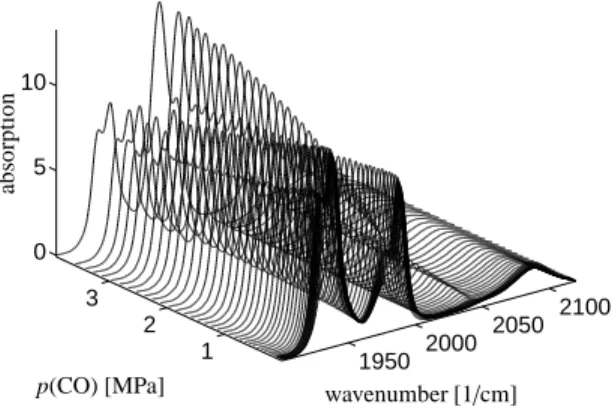
A detailed analysis of the equilibrium of iridium complexes for the hydroformylation of olefins has re- cently been published [12]. The equilibria of various hydridocarbonyltriphenylphosphine-iridium catalysts are analyzed at 373 K for varying partial pres- sure of carbon monoxide between p(CO)=10⁻²to 3.9 MPa at a constant hydrogen partial pressure of p(H2)= 1.0 MPa. The hydrido complexes were formed from Ir(COD)(acac), with c(Ir) = 5.0 ·10⁻³mol L⁻¹, and 10 equivalents of PPh3 under 2.0 MPa of synthesis gas [12]. Here we consider a sequence of k = 47 FT-IR spectra, and each spectrum is taken at n = 913 fre- quencies values in the interval [1900,2150]cm⁻¹. The sequence of spectra is shown in Figure 10.

The PGA has been applied three times in order to extract the three dominant components. A particular chal- lenge of this problem is that all pure component spectra are highly overlapping. The reconstruction is based on 11

(12)

18000 1850 1900 1950 2000 2050 2100 0.2

0.4 0.6 0.8 1

wavenumber [1/cm]

Spectrum of Rh(acac)(CO)₂

18000 1850 1900 1950 2000 2050 2100 0.5

1 1.5 2 2.5

wavenumber [1/cm]

Spectrum of Rh4(CO)12

1800 1850 1900 1950 2000 2050 2100 0

1 2 3 4 5

wavenumber [1/cm]

Spectrum of Rh6(CO)16

Figure 7: Results of a spectrum-by-spectrum computation with the PGA. The three selected channel windows are [2005.5, 2019.2] cm⁻¹, [1813.1,1822.5] cm⁻¹and [1872.1, 1894.4] cm⁻¹. These channel windows are marked by a gray background. All spectra are normalized so that the maximum in the window equals 1.

0 50 100 150 200 250 0

2 4 6

x 10⁻⁴

time [h]

Rh(acac)(CO)2

C(:.i) withυ^∗ C(:.i) with t⁺ C by global fit

0 50 100 150 200 250

0 1 2 3 4 5 6

x 10⁻⁴

time [h]

Rh4(CO)12

0 50 100 150 200 250

0 1 2 3

x 10⁻⁴

time [h]

Rh6(CO)16

Figure 9: Comparison of the three different approaches to compute C for the three pure components of the data set from Section 8.1. The global fit provides the best results (by the solution of the highest dimensional least squares problem). The local (windowed) reconstruction with (9) gives very similar results which shows that the PGA approach works very well. These two concentration profiles are much better thanCe=UΣt⁺by means of the pseudo-inverse t⁺. The latter approach which is associated with the solution of a least squares problem in a one-dimensional space results in a relatively poor approximation.

12

(13)

1950 2000 2050 2100 1

2 3 0 5 10

wavenumber [1/cm]

p(CO) [MPa]

absorption

Figure 10: Series of k=47 FT-IR spectra for an equilibrium mixture of iridium hydrido complexes registered during a variation of the carbon monoxide partial pressure, see Section 8.3.

the first z=3 left and right singular vectors. The channel windows and the weight factors are as follows (for the third windowω2 = 50 appears to be large, but all spectra are relatively smooth so that the contribution to the target function is small)

window ω1 ω2 γ1 γ2 γ3 γ4

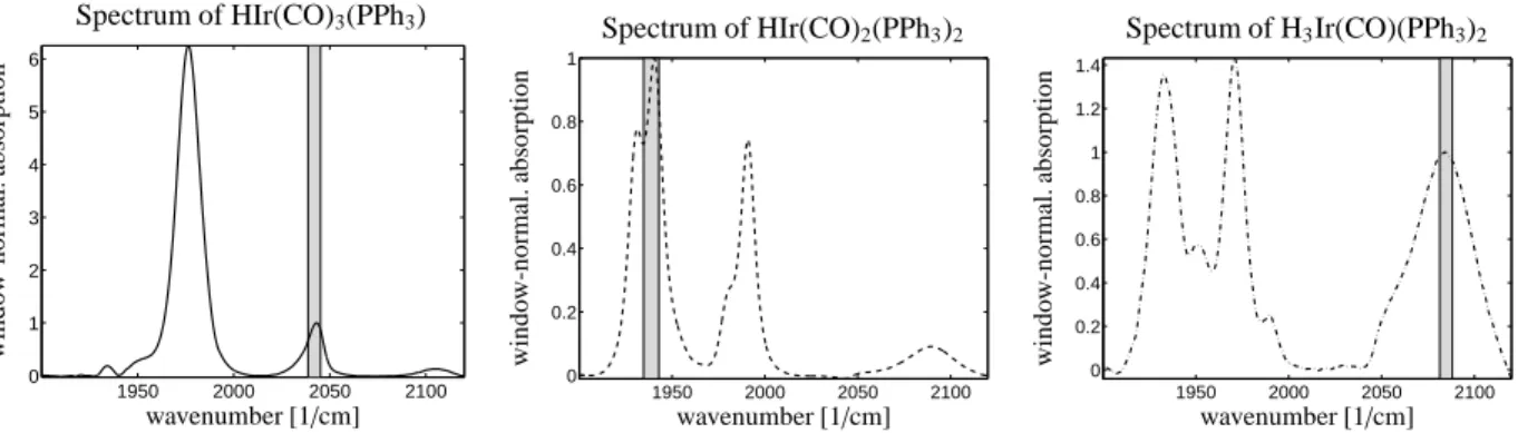
[2038.7,2045.2] 0.05 0 10 0.03 0 0 [1934.7,1942.9] 0.05 0 10 0.03 0 0.12 [2081.3,2088.1] 0.005 50 2 0.03 0 0 Three hydrido complexes have been identified, namely HIr(CO)₃(PPh₃), HIr(CO)₂(PPh₃)₂ and H3Ir(CO)(PPh₃)₂. The spectra for these three pure components are shown in Figure 11. Once again, the concentration profiles have been computed by solving a global least-squares problem on the full wavenumber interval since all three pure component spectra are available. The concentration profiles are shown in Figure 12.

8.4. PGA for weak peaks

In order to demonstrate the local amplification of weak peaks in the PGA the spectral data set from Sec- tion 8.1 is resumed. Now the wavenumber window [1980,1985] cm⁻¹is taken which is associated with the index interval I =[641,649], see Figure 13. The peak in this window is very small compared to the maximal absorption since

maxi∈ID(:,i) max D =0.02.

Once again a number of z=4 singular vectors are used.

For f1and f2the weights are set toω1=0.05 andω2=

0.5 1 1.5 2 2.5 3 3.5

0 0.5 1 1.5 2 2.5 3 3.5 4

x 10⁻³

p(CO) [MPa]

concentration profiles

HIr(CO)3(PPh3) HIr(CO)2(PPh3)2

H3Ir(CO)(PPh3)2

Figure 12: The pure concentration profiles for the three iridium complexes as computed by a global least-squares fit.

0. For the optimization the constraint functions g₁ and g₂ withγ₁ = 50 andγ₂ = 10 are active. The weight factors have a very different size due to the fact that the normalization (2) affects only g1but not f1and f2. What is finally found is the spectrum of the pure component Rh(acac)(CO)₂. The relative error of this solution called aweakcompared to the spectrum a1, see Section 8.1 and the leftmost sub-figure in Figure 7, is about 1.2% since

kαa_weak−a₁k₂ ka1k2

=0.012 with an optimized scaling parameterα=0.022.

9. Conclusion

The Peak Group Analysis (PGA) has been presented as a numerical algorithm which allows a step-by-step computation of the pure component spectra from the initial spectral data set for the chemical mixture. A crucial requirement for a successful application of the PGA is that certain single peaks or isolated peak groups can be identified whose spectral profile is dominated by a single pure component. Then this peak or peak group is the starting point for a local optimization procedure which results in a global spectrum of a pure component.

This global spectrum more or less reproduces the initial peak or peak group. The mathematical algorithm of the PGA is based on minimization of a target function to which various weighted soft constraints are added. We have also shown for experimental spectral data from the rhodium- and iridium-catalyzed hydroformylation process that the PGA is a useful tool for structure elucidation.

13