On the analysis and computation of the area of feasible solutions for two-, three- and four-component systems.

(1)

On the analysis and computation of the area of feasible solutions for two-, three- and four-component systems.

Mathias Sawallâ, Annekathrin Jürßâ, Henning Schröderâ, Klaus Neymeyrâ,b

aUniversit¨at Rostock, Institut f¨ur Mathematik, Ulmenstrasse 69, 18057 Rostock, Germany.

bLeibniz-Institut f¨ur Katalyse, Albert-Einstein-Strasse 29a, 18059 Rostock, Germany.

Abstract

The area of feasible solutions (AFS) is a low-dimensional representation of all possible concentration factors or spectral factors in nonnegative factorizations of a given spectral data matrix. The AFS analysis is a powerful methodology for the exploration of the rotational ambiguity inherent to the multivariate curve resolution problem. Up to now the AFS has been studied for two-, three- and four-component systems:

1. The AFS for two-component systems was introduced by Lawton and Sylvestre in 1971. For these two- dimensional problems the AFS can be constructed analytically.

2. For three-component systems the AFS can either be constructed geometrically (classical approach by Borgen and Kowalski from 1985) or it can be computed by numerical algorithms. Various computational techniques have been suggested by different groups in the recent past.

3. For four-component systems a first numerical method for its computation has been published recently. A new polyhedron inflation algorithm is under development.

In this review paper we explain the underlying concepts of the AFS theory and its contribution to a deepened un- derstanding of the multivariate curve resolution problem. A survey is given on various methods for the computation of the AFS for two-, three- and four-component systems. The focus is on methods which approximate the boundary of the AFS for three-component systems by inflating polygons and for four-component systems by inflating polyhe- drons. Several numerical examples are discussed and the MatLab-toolbox FACPACK for these AFS-computations is presented.

Key words: spectral recovery, factor analysis, nonnegative matrix factorization, area of feasible solutions, Generalized Borgen Plot, complementarity and coupling.

1. Introduction

Multivariate curve resolution techniques serve to extract the pure component information from multivariate (spectroscopic) data. Typically, the data is taken by spectral observation of a chemical reaction system on a time×frequency grid. If k spectra are measured, each at n frequencies, then the resulting matrix D is a k×n matrix. The measured data result from a superposition of the pure component spectra. Multivariate curve resolution methods can be applied in order to extract the pure component spectra and the concentration profiles.

The basic bilinear model underlying these methods is the Lambert-Beer law. In matrix notation, the Lambert- Beer law is a relation between D and the matrix factors

C∈R^k×sand A∈R^s×nin the form

D=CA. (1)

Therein s is the number of the pure or at least indepen- dent components. An error matrix E∈R^k×nwith entries close to zero can be added on the right-hand side of (1) in order to allow approximate factorizations in case of perturbed or noisy data D. In general, the matrices C and A are called abstract factors. One is interested in finding a factorization D = CA with chemically inter- pretable C and A. Then the columns of C∈R^k×sare the concentration profiles along the time axis of the pure components. And the rows of A ∈R^s×n are the associated pure component spectra.

The aim of a multivariate curve resolution (MCR) method is to determine the number s together with the

November 13, 2015

(2)

pure component factors C and A. Sometimes no addi- tional information on the pure components is available.

Then the MCR method only uses D for the pure compo- nent decomposition within a model-free approach. The main hurdle for any MCR technique is the so-called rotational ambiguity of the solution. See, e.g., [27, 28, 2]

for an introduction to the ambiguity problem. By apply- ing additional hard- or soft-constraints to the pure component factorization problem, one can often determine a single solution by means of a regularized optimization problem. In case of proper constraints this solution can be the chemically correct one. A large number of successful MCR methods has been developed.

Some examples are methods as MCR-ALS [19], RFA [29], SIMPLISMA [52], BTEM [7] and PCD [32]. Al- ternatively, one can give up the aim to determine only a single solution by solving a regularized optimization problem. Instead, one can follow the global approach of determining the full range of all nonnegative factoriza- tions D=CA with nonnegative rank-s matrices C and A. Such continua of possible nonnegative matrix fac- tors can graphically be presented either by drawing the bands of possible concentration profiles together with the bands of possible spectra [49] or by plotting these sets of feasible factors by a certain low-dimensional representation, the so-called Area of Feasible Solutions (AFS). The aim of this paper is to provide a systematic introduction to the AFS concept together with many references to the chemometric literature. Important properties of the AFS are presented together with computational techniques for its numerical approximation.

1.1. Organization of the paper

In the remaining part of this section, we introduce the four data sets which are used within this work. Section 2 explains in a compact form the principles of multivariate curve resolution methods and their relation to the singular value decomposition of the data matrix D.

The techniques to compute the factors C and A are ex- plained. In Section 3 the AFS and some of its important properties are described in detail. The rules for a classi- fication of feasible or non-feasible points are discussed in Section 5. In Section 6 methods for the computation of the AFS are explained with a focus on the polygon inflation method. Methods for the reduction of the AFS by using additional information or soft constraints are demonstrated in Section 8. In Section 9 we study dy- namic changes of the shape of the AFS under changes in the data (e.g. variation of a shift parameter). Finally in Section 10 the software package FACPACK for the computation of the AFS is pointed out.

1.2. Model data sets and experimental spectral data In this work we use four different data sets (two model data sets and two IR-spectroscopic data sets) for all demonstrations. The data sets are as follows:

Data set 1 (FT-IR experimental data on a Rhodium catalyst formation). This data set describes the two- component subsystem (s = 2) of the formation of a Rhodium catalyst from a certain precursor; for the un- derlying chemical problem see [24]. The data set in- cludes a number of k=977 spectra, each with n=481 wavenumbers. Within this spectral window the dom- inant absorbing components are a catalyst precursor and the catalyst. The usage of a first order reaction scheme allows to find unique factors C and A. These factors are shown in Figure 1. For the associated areas of feasible solutions see Figure 9.

Data set 2 (A three-component model problem). The consecutive reaction

X−^k→¹ Y −^k→² Z

is considered with the rate constants k₁ = 0.3 and k2 = 0.1. The initial concentrations are cX(0) = 1, cY(0) = cZ(0) =0 and the time interval is t ∈ [0,10].

The solution of the associated rate equations and its dis- cretization for a number of k=201 time steps results in the concentration matrix factor C∈R^201×3. The matrix factor A is derived from the three Gaussian functions aX(x)=exp −(x−30)²

1250+w

!

, aY(x)=exp −(x−50)² 1000+w

! ,

aZ(x)=exp −(x−70)² 1000+w

!

for x∈[0,100] and equidistant discretization along the frequency axis. A number of n=401 spectral channels is used. The spectra depend on the real parameter w which controls the signal width. The rows of the data matrix D as well as the original factors C and A for w = 0 are plotted in Figure 2. The associated areas of feasible solutions, namely the AFS for the concentra- tion factors C and the AFS for the spectral factors A, are presented in the first column of Figures 20 and 21.

See additionally the Figure 6 (with the data representa- tion in the leftmost plot) and Figure 15 for a successive approximation of the AFS by means of the polygon in- flation technique.

Data set 3 (Operando FT-IR specroscopic data from the Rhodium-catalyzed hydroformylation process). This data set is described in detail in [23]. The data consists 2

(3)

of k =850 spectra, each with n =642 wavenumbers.

The three major absorbing components form a reaction- subsystem and are an olefin component, a hydrido- complex and an acyl-complex. All these chemical com- ponents are explained in [23]. The series of mixture spectra and the factors C and A are shown in Figure 3. The Michaelis-Menten kinetic has been used as a ki- netic hard model in order to find unique concentration profiles. The complete set of all nonnegative factoriza- tions of the data matrix D is represented by the AFS for the concentration factor and by the AFS for the spec- tral factor. These AFS sets are plotted together with the associated bands of feasible solutions in Figure 7.

Data set 4 (A four-component model problem). The concentration factor C of this model problem results from solving the rate equations for the reaction scheme

W −^k→¹ X−→^k² Y −→^k² Z

with the kinetic constants k1 = 1, k2 = 0.25 and k3 = 0.1. The initial concentrations are cW(0) = 1, cX(0) = cY(0) = CZ(0) = 0 and the time interval is t ∈ [0,10]. The time-continuous concentration func- tions are discretized in k=26 time steps to form C.

The factor A derives from the Gaussian functions aW(x)=exp −(x−40)²

σ

!

, aX(x)=exp −(x−20)² σ

! ,

aY(x)=exp −(x−80)² σ

!

, aZ(x)=exp −(x−60)² σ

! , depending on the parameterσon the frequency interval x ∈ [0,100]. Numerical evaluation of these functions in n =31 equidistant channels results in the matrix A.

Thus the matrix A depends onσ. The mixture spectra, namely the rows of D =CA, are plotted together with the original factors C and A forσ =750 in Figure 4.

The associated areas of feasible solutions (concentra- tional and spectral AFS) are shown in Figure 19.

2. Multivariate curve resolution methods

Multivariate curve resolution methods are key-tools in order to extract the pure component information from the chemical mixture data in D. The problem is to com- pute

1. the number of independent components s and 2. the pure component factors C and A.

Any available information on the factors can and should be integrated into the MCR computations.

2.1. The singular value decomposition

The singular value decomposition (SVD), see [15], is a very powerful tool of numerical linear algebra to compute the left and right orthogonal bases for the ex- pansion of the pure component factors C ∈ R^k×s and A∈R^s×n; see for example [26, 28, 27, 38]. The SVD of D reads

D=UΣV^T.

Therein U ∈R^k×kand V∈R^n×nare orthogonal matrices whose columns are the left and right singular vectors.

The diagonal matrixΣcontains on its diagonal the singular valuesσ_iin decreasing order. The singular values are real and nonnegative. For an s-component system the first s singular vectors and the associated singular values contain all information on the system. For data not including perturbations only the first s singular val- ues are nonzero if the chemical system contains s inde- pendent chemical components. For data including noise some additional singular values are nonzero. In such cases the SVD allows to compute optimal (with respect to least-squares) rank-s approximations of D. If in the case of noisy data the noise-to-signal ratio is not too large, then the number of independent chemical com- ponents s can often be determined from the SVD. Then the relevant and meaningful singular values are clearly larger compared to the remaining nonzero singular values which evince the influence of noise, cf. [27, 32].

2.2. Reconstruction of the pure component factors The first s singular vectors, namely the first s columns of U and the first s columns of V, are used as bases to expand the desired pure component factors C and A.

For ease of notation we denote these submatrices of the SVD-factors again by U and V. Then U ∈ R^k×s and V ∈R^n×s. The matrices C and A are formed according to

C=UΣT⁻¹, A=T V^T. (2) Therein T ∈R^s×sis a regular matrix which remains to be determined. MCR methods typically provide a sin- gle pure component factorization D=CA and thus they explicitly or implicitly determine the matrix T . From C and A the matrix T of expansion coefficients is accessi- ble from Equation (2). For SVD-based MCR methods see [26, 28, 27, 32] and the references therein.

The basis expansion approach (2) drastically reduces the number of free variables of the pure component factorization problem. The crucial point is that the number of matrix elements of C and A is (k+n)s whereas the 3

(4)

1 50 100 0

0.2 0.4 0.6 0.8 1

channels

absorption

Data D

0 0.2 0.4 0.6 0.8 1

time

concentration

Concentration profiles

1 50 100

0 0.2 0.4 0.6 0.8 1

channels

absorption

Pure component spectra

Figure 1: Data set 1: The series of mixture spectra is shown left (only every tenth spectrum of the data is plotted). All ordinate axes are scaled to a maximum of 1 and the channel windows are set to [1, . . . ,100]. By enclosing a kinetic hard-model for the reaction scheme (X→Y) into the pure component decomposition unique matrix factors (aside from the multiplicative ambiguity and the permutation ambiguity) have been determined.

These are shown in the centered and right subplot.

0 20 40 60 80 100

0.2 0.4 0.6 0.8 1

channels

absorption

Data D

0 2 4 6 8 10

0 0.2 0.4 0.6 0.8 1

time

concentration

0 20 40 60 80 100

0.2 0.4 0.6 0.8 1

channels

absorption

comp. X comp. Y comp. Z

Figure 2: Data set 2 for w=0: The leftmost plot shows the series of the mixture spectra, i.e. the rows of the matrix D. Only every third spectrum of the data is plotted. The remaining two plots show the concentration profiles and the spectra of the three pure components.

2000 2050 2100

0 0.02 0.04 0.06

wavenumbers [cm⁻¹]

absorption

Data D

0 200 400 600 800

0 0.02 0.04 0.06

time [min]

unscaledconcentration

2000 2050 2100

0 0.2 0.4 0.6 0.8 1

wavenumbers [cm⁻¹]

normalizedabsorption

olefin hydrido-complex acyl-complex

Figure 3: Data set 3 on catalyst formation within the hydroformylation process: The leftmost subplot shows the spectral data, i.e. the rows of D.

Only every tenth spectrum of the data is actually plotted. The remaining two subplots show the concentration profiles and the spectra of the pure components. For a successful pure component decomposition of these spectral data a Michaelis-Menten kinetic hard-model has been integrated into the pure component factorization.

0 20 40 60 80 100

0.2 0.4 0.6 0.8 1

channels

absorption

Data D

0 2 4 6 8 10

0 0.2 0.4 0.6 0.8 1

time

concentration

0 20 40 60 80 100

0.2 0.4 0.6 0.8 1

channels

absorption

comp. W comp. X comp. Y comp. Z

Figure 4: Data set 4 forσ=750: The spectral data (left) for the four-component model problem together with the concentration profiles of the pure components (center) and the pure component spectra (right).

4

(5)

representation by Equation (2) reduces the degrees of freedom to the s²matrix elements of T . Hence the rep- resentation (2) is a basic ingredient for the construction of computationally effective MCR methods.

2.3. Application of hard- and soft constraints

Hard- and soft constraints have a crucial role in the construction of MCR methods [16, 11, 51, 32, 42]. A very restrictive and often successful hard constraint is a kinetic model of the underlying chemical reaction system. Only those concentration factors C are ac- ceptable which are consistent with the kinetic model [8, 20, 27, 39]. Typically, the rate constants are implicitly computed as a by-product of the model fitting process.

If no kinetic model is available for C, then soft con- straints can be used in order to extract (from the set of all nonnegative factorizations) solutions with special properties, see e.g. [16, 11, 51, 32, 42]. Typical examples of such soft constraints are those on the smoothness of the concentration profiles in C or A, constraints on a small or large integral of the spectra in A (in order to favor solution with few and sharp peaks or alternatively those with a large number of wide peaks), criteria on the closure of the concentration data and so on. Such soft constraints are usually added to the reconstruction functionalkD−CAk²_F in terms of a cost function

g(T )=

p

X

i=1

γ_ikg_i(C,A)k²₂.

According to the representations of C = C(T ) and A =A(T ) as functions of T , the cost function g(T ) in- cludes a number of p constraint functions gi. Theγi≥0 are the associated weight factors which give the user the possibility to determine a certain balance between the different constraints. A small reconstruction error kD−CAk²_F together with the nonnegativity of the fac- tors C and A is of highest importance; sometimes small negative entries in C and A can be acceptable. Other constraint functions are of lower importance, e.g. on the smoothness. For these constraint functions smaller weight factorsγ_iare used.

3. The area of feasible solutions

Even with proper constraint functions and proper weight factors, MCR methods cannot always find the chemically correct or “true” solution. Thus one might follow the alternative idea to determine the set of all nonnegative factorizations D = CA. Such solutions

which only fulfill the nonnegativity constraint are called feasible or abstract factors. The global approach of computing all feasible factors provides an elegant way in order to survey the complete rotational ambiguity of the pure component factorization problem. However, the sets of feasible matrices C ∈ R^k×sor A ∈R^s×nare difficult to handle. The key idea to make these sets of feasible factors accessible is their low-dimensional rep- resentation in terms of the so-called Area of Feasible So- lutions (AFS). The AFS refers to the representation of C and A as functions of T by Equation (2). Only a single row of T is sufficient to represent a feasible factor, see Section 3.2 for the details. In the following, our analysis aims at determining the AFS for the spectral factor A starting from a spectral data matrix D. This analy- sis can immediately be used to determine the AFS for the concentrational AFS containing the feasible factors C. Therefore we apply the procedure to the transposed data matrix D^Tsince in D=CA the factors change their places by the transposition D^T =A^TC^T.

The aim of this section is to introduce the AFS and to discuss some of its important properties. We consider especially those properties which are decisive for an effective numerical computation of the AFS.

3.1. Development of the AFS concept and discussion of methods for its numerical computation

In this section a short overview is given on the development of the AFS concepts. These developments are closely related with the growth of effective numerical methods for its computation.

The AFS for two-component systems was first analyzed by Lawton and Sylvestre in 1971, see [26]. The Lawton-Sylvestre plot is a 2D plot of the set of the two expansion coefficients (with respect to the basis of singular vectors) which result in nonnegative matrix factors C and A. The Lawton-Sylvestre plot for a two compo- nent system consists of two cones whose boundaries can be computed analytically, see [50, 1, 35] and Section 4.

For three-component systems a direct analogue of the Lawton-Sylvestre plot would be a three-dimensional plot of feasible expansion coefficients. Such three- dimensional objects are somewhat more complicated to draw, to handle and to understand. However, there is a tricky dimension reduction (by a certain scaling) which allows to represent these AFS sets for three-component systems only by two expansion coefficients (and thus by plots in 2D). This was suggested by Borgen and Kowal- ski, who published in 1985 [6] a geometric construction of these 2D AFS plots for three-component systems. These plots are called Borgen plots. The mentioned dimension reduction can be explained by a typ- 5

(6)

ical Lawton-Sylvestre plot which is shown in Figure 5.

For a two-component system the Lawton-Sylvestre plot consists of two cones. If the first expansion coefficient t₁is fixed to 1, then the intersection of the dash-dotted line at t1=1 with the two cones are two separated intervals. These two intervals are a 1D analogue of the Bor- gen plots. For a three-component system the 2D Borgen plot is the two-dimensional intersection of a plane at t1

with a 3D generalization of a Lawton-Sylvestre plot.

The geometric construction of the Borgen plots is deepened by further concepts in [36] and [22]. In addi- tion to the geometric constructions of the Borgen plots, various techniques for a numerical approximation of the AFS for (s=3)-component systems have been devised.

These are the grid search method (for two-component systems in [50, 1]), the triangle enclosure method [12]

and the polygon inflation method [43, 44]. One bene- fit of the numerical methods compared to the geometric methods is that the numerical methods are able to compute the AFS in the presence of noise. Recently, the classical geometric construction has been generalized in a way which allows geometric AFS constructions for noisy data [22].

For systems with more than three components the problem of AFS computations is more complex and requires large computation times. For 4-component systems a generalized triangle enclosure method which uses a slicing of the 3D AFS has already been published [14]. The basic grid search algorithm and the polygon inflation method can also be extended to such higher dimensional problems.

AFS computations can be used to determine the so- called feasible bands. To this end, one can draw the con- tinua of concentration profiles or the continua of possible spectra which are represented by the AFS. The resulting feasible bands visualize the rotational ambiguity.

The MCR-Bands toolbox [49, 21] pursues the same ob- jective, namely to construct the feasible bounds. How- ever, the MCR-Bands approach does not require a previ- ously constructed AFS. Instead, the band boundaries are constructed by a minimization respectively maximiza- tion of a properly constructed target function.

3.2. The set of feasible pure component spectra Our focus is on the construction of the set of all possible pure component spectra. The set of feasible concentration profiles can be computed similarly; therefore the computational procedure is to be applied to D^T. The permutation of the columns of C and the same permuta- tion applied to the rows of A does not provide any new information. This fact is known as the (trivial) permutation ambiguity. A consequence of this property is that

the problem to find all feasible factors A is equal to the problem to determine the set of all first rows of the feasi- ble factors A. Hence the set of feasible pure component spectra (also called feasible bands) for an s-component system reads

A={a∈Rⁿ : exist C,A≥0 with A(1,:)=a

and D=CA}. (3)

For the computation ofAwe prefer the SVD-based approach (2). A further reduction of the degrees of freedom is possible. This is explained next.

3.3. Reduction of the degrees of freedom

Equation (2) is a representation of the s×n matrix A by the matrix T with only s²matrix elements. These s² matrix elements are the expansion coefficients with respect to the basis of right singular vectors. As shown for the derivation of (3) only the first row of A=T V^Tis required in order to form the setAof feasible spectra.

The first row of A equals the first row of T V^T. Hence only the s matrix elements of the first row of T are deci- sive. This reduces the degrees of freedom from s²down to s.

These remaining s degrees of freedom for an s- component reaction system can further be reduced to s−1 by a certain scaling of the rows of A. In [6, 36]

thek · k1vector norm (i.e. the sum of the absolute values of the components) is used for the normalization of the spectra. Alternatively, the maximum normk · kmaxcan be used. Here we follow the approach in [12, 14, 43, 44]

and use a scaling which sets the first column of T equal to ones, i.e.

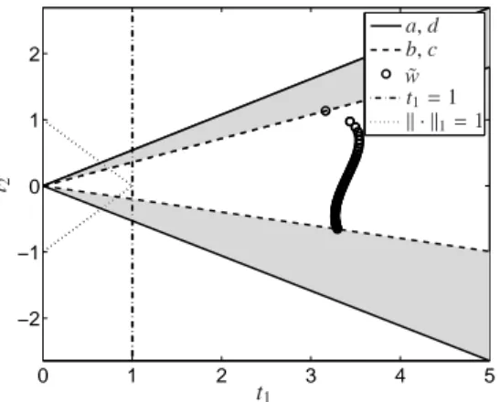
T (i,1)=1 for all i=1, . . . ,s. (4) This can be called the first-singular-vector scaling (FSV- scaling) since it uses for the first right singular vector the fixed expansion coefficient 1. A precise justification for this choice is based on the Perron-Frobenius theory [30] on spectral properties of nonnegative matrices; for the details see Theorem 2.2 in [44]. Figure 5 shows a typical Lawton-Sylvestre plot for a two-component model problem. The dash-dotted and the dotted lines define two intersections with the Lawton-Sylvestre plot.

These intersections are the 1D AFS representations with respect to the FSV-scaling and with respect to thek · k1

normalization.

6

(7)

0 1 2 3 4 5

−2

−1 0 1 2

t1

t2

a, d b, c

˜ w t₁=1 k · k₁=1

Figure 5: The Lawton-Sylvestre plot (gray triangle-shaped areas) for a two-component model problem. The dash-dotted and the dotted lines define two intersections with the Lawton-Sylvestre plot. These intersections are the 1D AFS representations with respect to the FSV- scaling and with respect to the k · k1 normalization. The points

˜

w(i,:) =D(i,:)V(:,1 : 2), i=1, . . . ,n, are drawn by small circles.

These points represent the rows of D. Mathematically the coordinates of these points are the expansion coefficients of the rows of D with respect to the two dominant right singular vectors. For a more de- tailed explanation of the AFS and for the meaning of a, b, c and d see Section 4.

3.4. Definition of the AFS

With respect to the FSV-scaling (4) the matrix T in (2) has the form

T =







1 x1 · · · xs−1

1

...

S

1







. (5)

Therein S is an (s−1)×(s−1) matrix. Only the s−1 el- ements of the row vector x=(x1, . . . ,xs−1) are decisive for the representation of the set of all feasible solutions.

With these definitions the setA ⊂Rⁿby Equation (3) can be represented by the associated set of expansion vectors x ∈ R^s−1. Such a set of (s−1)-dimensional vectors for a chemical reaction system with s species is much easier to handle compared to the subsetAof the higher dimensional spaceRⁿ. The set

M={x∈R^s−1: exists S so that T in (5) fulfills rank(T )=s and C,A≥0} (6) is called the AFS for the factor A or the spectral AFS.

Figure 6 shows a typical AFS for the three- component underlying the data set 2. This AFS consists of three isolated subsets. In [43, 44] these subsets are called segments of an AFS. Further, two series of points are marked within two segments of the AFS. The associated series of spectra, which are represented by these

points, are also shown in Figure 6. Figure 7 displays the AFS sets of the factors C and A for the data set 3. Addi- tionally, this figure shows the associated bands of feasible pure component spectra, i.e. the setA. The feasible bands of concentration profiles are also plotted; this set results from computing the setAfor the transposed data matrix D^T.

3.5. Properties of the AFS

The AFS has several interesting properties. Many of these properties derive from the Perron-Frobenius spectral theory of nonnegative matrices [30]. This theory provides (see Section 3.3) the justification for the scaling condition (4). An important property of the AFS is its boundedness, see Section 3.5.2. This property makes possible a numerical approximation of the boundary of the AFS. The AFS sets may have several shapes. For three-component systems the most important cases are AFS sets which consist of three separated segments and AFS sets which have the form of a topologically connected set with a single hole. Such a hole always contains the origin (null vector), see, e.g., Figure 24 and Section 3.5.3. Further explanations on the geometric construction of the AFS and its relationship to the theory of simplices and convex combinations are contained in [36, 22].

3.5.1. Definition of FIRPOL and INNPOL

For the further analysis the two polygons FIRPOL and INNPOL are to be introduced. First, the set

M⁺={x∈R^s−1: (1,x)V^T ≥0} (7) is called FIRPOL [6, 36, 22]. All points x inM⁺result in nonnegative linear combinations of the right singular vectors, i.e. (1,x)V^T. Thus FIRPOL is a superset of the set of feasible spectra. The membership of a certain x to M⁺does not guarantee that the nonnegative spectrum (1,x)V^T is part of a feasible pure component decompo- sition D =CA. The crucial point is that nonnegativity of (1,x)V^Tdoes not necessarily imply the nonnegativity of an associated concentration profile.

Further, the setM^∗is to be introduced

M^∗={x∈R^s−1: exists S so that T in (5) fulfills rank(T )=s and C≥0, A(2 : s,:)≥0}. (8) The two setsM⁺andM^∗are super-sets of the AFSM.

The definition ofM⁺includes only the nonnegativity- constraint A(1,:) ≥ 0. The definition ofM^∗ includes 7

(8)

−1 −0.5 0 0.5 1

−0.2 0 0.2 0.4 0.6 0.8 1

x1

x2

AFS for A and sequences of points

0 20 40 60 80 100

0

channels

Reconstructed spectra for×

0 20 40 60 80 100

0

channels

Reconstructed spectra for◦

Figure 6: Data set 2 Left: The spectral AFS for this three-component system consists of three isolated subsets. In two of these subsets sequences of points are marked. The points marked by×have a color shading from red to black. The points marked by◦have a color shading from green to black. The associated series of spectra are shown in the same color shading in the remaining two subplots.

−1 −0.5 0 0.5

−0.6

−0.4

−0.2 0 0.2 0.4 0.6

AFS for factor C

−0.5 0 0.5 1

0 0.5 1

AFS for factor A

200 400 600 800

0

time [min]

Feasible bands for factor C

2000 2050 2100

0

wavenumbers [cm⁻¹] Feasible bands for factor A

Figure 7: Data set 3: The areas of feasible solutions, namely the AFS for the concentration factor C and the AFS for the spectral factor A, are plotted (left) together with the associated bands of feasible solutions (right).

the remaining constraints on nonnegativity and the rank condition. ThusM=M⁺∩ M^∗. Finally, the vectors

w(i,:)=D(i,:)V(:,2 : s)

D(i,:)V(:,1) ∈R^s−1for i=1, . . . ,n (9) are introduced. In [6, 36, 22] the convex hull of these points w(i,:), i=1, . . . ,n, is called INNPOL [6, 36, 22].

3.5.2. Boundedness of the AFS

Three numerical approximation methods for the com- putation of the AFS for two- and three-component system have been described in literature. These are the grid search algorithm [50], the triangle enclosure method [12] and the polygon inflation method [43]. In order to guarantee that these algorithms terminate within finite times, the boundedness of the AFS is required. Theo- rem 2.4 in [44] proves thatM⁺is a bounded set if and only if D^TD is an irreducible matrix. Thus the AFS Mis also a bounded set sinceM ⊂ M⁺. See [30] or [44] for the definition of an irreducible quadratic matrix. Practically, irreducibility is always guaranteed if the whole system does not allow a complete separation into two independent subsystems. The latter case is al-

ready a trivial case as completely isolated subsystems can be analyzed separately.

3.5.3. The origin is never included in the AFS

As already mentioned in Section 3.5 the origin (or null vector) is never contained in the AFS. The proof for this fact is given in Theorem 2.2 in [44]. It is based on the Perron-Frobenius theory and uses the irreducibil- ity of the matrix D^TD. For the cases that the AFS consists of several isolated subsets, called segments, these subsets do not contain any holes. In mathematics such sets are called simply-connected. The approach of in- flating polygons can be used in order to approximate such AFS segments. The remaining case that the AFS consists of only a single set is more complicated. Such a single-segment AFS always contains a hole and this hole encloses the origin. The inverse polygon inflation algorithm is a modification of the polygon inflation algorithm which allows a fast and accurate numerical approximation of such one-segment AFS sets with a hole.

See Section 4 in [44] for the details.

8

(9)

3.5.4. Geometric AFS construction

The geometric construction of the AFS for three- component systems was introduced by Borgen and Kowalski in 1985 [6, 5], see also [36, 22]. The resulting geometric constructions are called Borgen plots.

The construction principles of Borgen plots are not limited to s = 3 but can be applied to general s- component systems. In the general case a point x is feasible if and only if there exist further s−1 points y_j, j = 1. . . ,s−1, so that the simplex spanned up x and the vectors y_j is enclosed inM⁺ and includes all points w(i,:) given by Equation (9). These points are the vertices of INNPOL. Consequently the classical theory by Borgen and Kowalski works with convex equa- tions. A weakening from convex combinations towards affine combinations allows to generalize the geometric AFS construction [22]. The resulting generalized Bor- gen plots can be constructed even for noisy or perturbed spectral data.

3.6. Segment structure of the AFS

For two-component systems and with respect to the FSV-scaling, the AFS (6) always consists of two separated 1D intervals. The intervals may degenerate to single points. One of these intervals is completely negative and the other one is completely positive, see Figure 8 and in Figure 5 the cross-section at t1=1.

For three-component systems the AFS can consist of a single segment with a hole around the origin or of a number of 3m segments for m = 1,2, . . .. A formal proof is planned for a forthcoming paper. For experimental data sets only the cases of a one-segment AFS and of 3-segment AFS sets have been observed. Only these cases appear to be practically relevant. However, nonnegative matrices D can be constructed whose asso- ciated AFS sets consist of 6, 9, . . . separated segments.

For s-component systems with s ≥ 4 little information exists on the possible numbers of segments.

By changing the data D continuously one can explore the resulting changes of the associated AFS sets. How- ever, such parameter dependent data sets could hardly be found as experimental data sets. The data sets 2 and 4 in Section 1.2 include the parameters w andσ. For each of these data sets a variation of these parameters allows to start from AFS sets with either 3 or 4 separated segments and to end in one-segment AFS sets each with a hole. See Figure 24 for the AFS-dynamics in case of the data set 2 and Figure 25 for the data set 4.

4. The AFS for two-component systems

The AFS for systems with a number of s=2 components can explicitly be described analytically. The numerical evaluation of the analytic formula results in the 1D AFS plots. Next these formula are compiled. The starting point for the case s = 2 is the matrix T by (5) which together with its inverse read

T = 1 x

1 S₁₁

!

, T⁻¹= 1

S11−x

S₁₁ −x

−1 1

! . The nonnegativity for the factors C and A results in fea- sible intervals for x and S11, see also Section 3.6 in [44]

and [1]. With a=− min

i with V(i,2)>0

V_i1 Vi2

, d=− max

i with V(i,2)<0

V_i1 Vi2

, b=min

i

Ui2σ2

Ui1σ1

, c=max

i

Ui2σ2

Ui1σ1

(10)

the AFS for the two-component system has the form of two separated intervals

M=[a,b]∪[c,d]. (11) This result can be interpreted in a way that both

x∈[a,b] and S11∈[c,d]

and

S₁₁∈[a,b] and x∈[c,d]

result in nonnegative factors.

A certain choice

(x,S11)∈[a,b]×[c,d]

completely determines a nonnegative factorization D= CA. The second choice (S11,x)∈[a,b]×[c,d] does not provide any new information. Instead, the second solution is equal to the first solution after a row permutation in A and a column permutation in C. This fact justifies that the AFS for two-component systems is often repre- sented by the rectangular [a,b]×[c,d], see [50, 1, 44].

4.1. Numerical AFS computation for the data set 1 For noisy or perturbed spectral data it can be ad- vantageous to accept small negative entries in the pure component factors. With a positive control parameter ε on the tolerated size of negative entries of C and A (see Section 5.1) one can generalize the AFS-bounds as discussed above. Next numerical results generated by the FACPACK software [45] are presented for the two- component experimental FT-IR spectroscopic data set 9

(10)

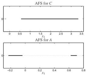
0 0.5 1 1.5 2 2.5 3 3.5 0

−0.2 0 0.2 0.4 0.6 0.8

0

x1

AFS for C

AFS for A

Figure 8: Data set 1: The AFSMfor this two-component system for the concentrational factor (upper plot) and for the spectral factor (lower plot). The control parameterεon acceptable negative entries readsε=0.035.

1 2 3

−0.21

−0.2

−0.19

−0.18

Rectangle-AFS for C

−0.2 −0.15 −0.1 −0.05 0.62

0.64 0.66 0.68 0.7 0.72

Rectangle-AFS for A

Figure 9: Data set 1: Two-dimensional rectangle representation of the 1D-AFS in which the two intervals of the one-dimensional AFSM are the edges of a rectangular. A certain point (with the two coordi- nates x and S11) completely determines either C and A. The control parameter is againε=0.035.

1. Figure 8 shows the one-dimensional AFS sets with ε = 0.035 for the concentrational factor C and for the spectral factor A. Additionally, Figure 9 shows for the same problem the two-dimensional rectangle representation of the same AFS. The two intervals of the one- dimensional AFS form the edges of a rectangular. The advantage of such a rectangle-representation is that a certain point (with the two coordinates x and S11) com- pletely determines C or A. Moreover, a known factor C allows to compute A from D=CA and vice versa.

5. Feasibility of points in the AFS

For the case of two-component systems the question of the feasibility of a certain point is solved by the analysis in Section 4 (at least for noise-free data). In the following we consider systems with three or more components. For these systems the feasibility question arises in two major ways. There is first the feasibility analysis

for noise-free (model) data by considering a certain geometric construction. Alternatively, and with a focus on experimental spectral data, there is a numerical feasibility analysis which is based on the numerical solution of an optimization problem. Unfortunately, the numerical feasibility test can yield false results, if the numerical optimization procedure (e.g. due to convergence problems or poor initial estimates) is not successful.

This section explains the feasibility checks of the polygon inflation algorithm by soft constraints (in the Subsection 5.1), of the triangle enclosure technique as well as the grid search method (see Subsection 5.2) and of the geometric-constructive Borgen plot approach (see Section 5.3).

5.1. Soft-constraint based feasibility check

Soft constraints can be added to the feasibility check on nonnegativity. The aim of this approach is to com- pute the matrix elements of the submatrix S of (5) by solving a minimization problem for a certain target function which guarantees that CA is a good approxi- mation of the initial matrix D. Simultaneously various constraints on C and A are to be satisfied. This fea- sibility test which also underlies the polygon inflation algorithm [44] is explained in the following.

First we introduce a small control parameterε ≥ 0 so that−εis a lower bound for the acceptable negative elements of C and A (in a relative sense related to the maximal value of a concentration profile or spectrum).

Mathematically, these conditions read minjC( j,i)

maxjC( j,i) ≥ −ε, minjA(i,j) maxjA(i,j) ≥ −ε for all i = 1, . . . ,s. The acceptance of small negative entries can often significantly stabilize the computation in case of noisy or perturbed (e.g. by a background subtraction) data.

The feasibility test for a point x is done in two steps.

First, a rapid and computationally very cheap test is used in order to check whether x is contained in the set FIRPOLM⁺, see Equation (7). If x is not in FIRPOL, then x cannot be an element of the AFSM. Once again, we accept small negative entries. To this end we use an approximate FIRPOL test in order to check whether or not

f₀(x) :=min (1,x)V^T

k(1,x)V^Tk_∞ +ε, 0

!

(12) satisfies that f₀(x) ≥ 0 (in a component-wise sense).

Therein,k·k∞is the maximum vector norm, which is the largest absolute value of all components of its argument.

10

(11)

−1 −0.5 0 0.5 1 0

0.5 1 10⁻⁶ 10⁻⁴ 10⁻² 10⁰

x1

x2

kf0(x)k+minS∈R2×2f(x,S)

Figure 10: Data set 2: The functionkf0(x)k+minS f (x,S ) is plotted.

The valley bottom is the AFS.

If this test is passed successfully, then a second much more expensive test follows. Therefore the soft constraint function

f (x,S )=

s

X

i=1

min C(:,i) kC(:,i)k∞

+ε, 0

!

2

F

+

s

X

i=2

min A(i,:)

kA(i,:)k_∞ +ε, 0

!

2

F

+kI_s−T T⁺k²_F (13)

is considered with T=T (x,S ) by (5). Further, C, A are computed according to (2). If

min

S∈R(s−1)×(s−1) f (x,S )≤εtol, (14)

then x has passed the feasibility test successfully.

Therein εtol is a small positive control parameter, e.g.εtol=10⁻¹⁰.

To summarize, the approximate feasibility test with the control parametersεandεtolresults in the (approximate) AFS

M={x∈R^s−1: x fulfills f0(x)≥0 and min

S f (x,S )≤εtol}. (15) Figure 10 shows the functionkf0(x)k+minS f (x,S ) on the grid (x1,x2) ∈ [−1.2,1.2]×[−0.4,1.4] for the data set 2. For these computations the control parameters areε = 10⁻¹² andε_tol = 10⁻⁶. All points with kf₀(x)k+min_S f (x,S )≤10⁻⁶belong to the AFS; these are the points at the valley bottom in Figure 10.

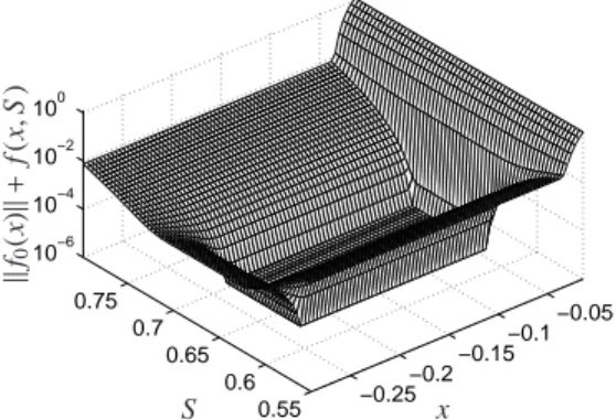
For the data set 1, a two-component system, Figure 11 displays the functionkf₀(x)k+ f (x,S ) on the grid (x,S ) ∈ [−0.29,−0.01]×[0.55,0.8] for ε = 0.035.

For this two-component system no minimization is re- quired; the arguments S and x of f are real numbers.

−0.25−0.2−0.15

−0.1−0.05

0.55 0.6 0.65 0.7 0.75 10⁻⁶ 10⁻⁴ 10⁻² 10⁰

x S

kf0(x)k+f(x,S)

Figure 11: Data set 1: The functionkf0(x)||+f (x,S ) with scalar ar- guments x and S is plotted. The control parameterεis set to 0.035 in order to successfully deal with small negative entries which are caused by a baseline correction. Since f (x,S )= f (S,x) the function graph ofkf0k+f is symmetric to the axis x=S ; the symmetric part of the function is not plotted. The area withkf0(x)k+minS f (x,S )< εtolis bounded by the interval endpoints a, b, c and d as given in Equation (10).

The valley bottom is equal to the right subplot of Fig- ure 9. The endpoints of the intervals are approximately equal to a and b in (10) and are located on the x1-axis.

Further the endpoints c and d are located on the S -axis.

5.2. The ssq-function based feasibility check

The ssq-function (ssq for sum-of-squares) approach evaluates the reconstruction functional

ssq(x,S )=kD−max(C,0)·max(A,0)k²_F. Therein max(C,0) and max(A,0) are the matrices whose negative entries are zeroed. The matrices C and A de- pend on T = T (x,S ) according to (5). The triangle enclosure algorithm [12] and the grid search method [50, 1] are based on the evaluation of the ssq-function.

Computationally, the ssq-evaluation is relatively expen- sive as the computation ofO(k·n) squares is required whereas the evaluation of (13) needs only O(k+ n) squares. For large numbers k and/or n this results in significantly different computation times; see for example Tables 1 and 2 in [44] for a direct comparison of the soft constrained approach (13) compared to the ssq- based AFS computation.

Finally, the AFS can be written as M=

x∈R^s−1: min

S ssq(x,S )≤εtol

for a fixed small parameterεtol>0.

5.3. Geometric constructive feasibility test

The fundamentals of the geometric AFS construction are shortly outlined in Section 3.5.4. Principally, these 11

(12)

constructions are not limited to (s=3)-component systems. However, the current literature does not contain any investigations for s≥4.

The geometric feasibility test of a certain point x ∈ M⁺for the case s =3 amounts to the following steps:

First two tangents of INNPOL are constructed which run through the given point x and which (tightly) en- close INNPOL. Next the intersection of the first tangent with the boundary ofM⁺(the line segment between x and this point must touch at least one point w_i) is de- fined as P₁. The same is done for the second tangent.

This results in the point P₂. Then x is a feasible point of the AFS if and only if the triangle with the vertices x, P₁ and P₂ includes the polygon INNPOL, see Sec- tion 3.5.1. An extension of this geometric construction which is applicable to noisy or perturbed data is developed in [22].

6. AFS computations for three-component systems The definition of the AFS and the discussion of some of its numerous properties is now followed by a numerical algorithm for its computation. The focus is on the polygon inflation algorithm [43, 44] and its implemen- tation in the FACPACK software. We also briefly dis- cuss the geometric AFS construction, the triangle enclosure algorithm, the grid search approach and the MCR- Bands method for the computation of upper and lower band boundaries. We do not claim to present a complete discussion of all methods for AFS computations.

For example, we do not consider the particle swarm algorithm for the detection of feasible regions [48].

6.1. Borgen plots and computational geometry

The geometric construction of Borgen plots has already been introduced in Section 3.5.4. This construction is purely geometric [6, 36]. The practical imple- mentation of the construction on a computer requires methods of computational geometry. Hence a floating- point arithmetic is used so that certain approximation problems can occur. Perturbed spectral data, data which result from an SVD low rank approximation or spectral data containing small negative entries (e.g. from background subtraction) cannot successfully be treated with the classical Borgen plots. In [22] a generalized Bor- gen plot construction has been suggested which has extended the construction principles to perturbed spectral data. Generalized Borgen plots can be constructed with the FACPACK software.

6.2. Grid search

The grid search approach [50, 1] is a brute-force method to compute the AFS. It can be used for any s≥2. For two-component systems the function f (x,S ) is plotted on a proper grid inR², see Section 4.1 or Fig- ure 8. For the cases s≥3 one has to evaluatekf0(x)k+ minS f (x,S ) by Equation (13) or minS ssq(x,S ) on a suitable grid. Figures 11 and 10 show the function graphs for the data set 2 and for the data set 1. The grid search method can simply be implemented on a computer. However, the computational costs increase expo- nentially in the number of components s. Moreover, the grid search approach is a non-adaptive method. Any increase of the resolution by a factorκ(e.g., in each coor- dinate direction the number of grid points is multiplied byκ) results in an increase of the computational costs by the factor ofκ^s−1.

6.3. Triangle enclosure

The triangle enclosure method was introduced in 2011 for three-component systems in [12]. The idea is to approximate the boundary of the two-dimensional AFS by series of equilateral triangles which cover the boundary. Therefore an initial triangle is computed for which at least one vertex x fulfills that x ∈ M and at least one vertex y is not located inM. The third point z can be a feasible or a non-feasible point. Then the generation of further triangles starts. The idea is to mir- ror the most recently generated triangle along one of its edges which intersects the boundary ofM. This is done in a way that the triangle chain grows until the initial triangle is reached. Then the boundary of a segment of the AFS has been successfully approximated.

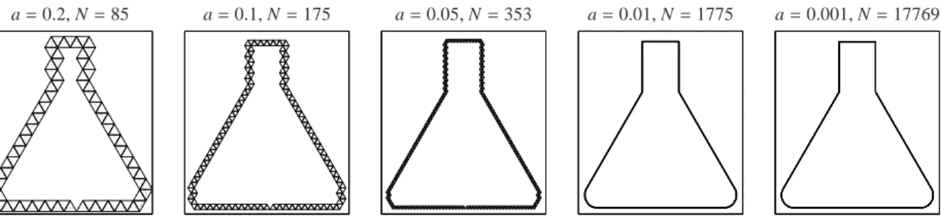
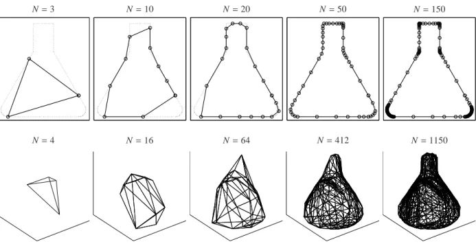
Figure 12 illustrates the idea of the triangle enclosure method. The shape of an Erlenmeyer flask is approximated by a chain of equilateral triangles. This is done for different edge lengths a. The precision of the bound- ary approximation is equal to the edge length a. Halving the edge length in order to increase the approximation quality doubles the number of required triangles.

For each segment (or isolated subset) of the AFS a separate chain of triangles is to be computed, see Sec- tion 3.5 for the possible cases. However, if the AFS consists of only a single topologically connected set, then this set contains a hole which encloses the origin. In this case an additional run of the triangle enclosure algorithm is required in order to approximate the inner boundary by a second chain of triangles. The computational costs of the triangle enclosure algorithm is significantly smaller compared to the grid search method.

The reason is that feasibility tests are only required for points close to the boundary.

12

(13)

a=0.2, N=85 a=0.1, N=175 a=0.05, N=353 a=0.01, N=1775 a=0.001, N=17769

Figure 12: Approximation of the shape of an Erlenmeyer flask by the triangle enclosure method by chains of equilateral triangles with edge lengths a. The required number of triangles is N. The start triangle is chosen in the way, that its centroid is located in the middle of the bottom-line. The edge length a limits the precision of the boundary approximation.

6.4. MCR-Bands

The MCR-Bands method [10, 49, 21] is not gener- ically an AFS computation method. Instead, MCR- Bands aims at the computation of lower and upper boundaries for the feasible bands of each component.

The method works for any s≥1. The band boundaries are computed by minimizing (for the lower boundaries) or maximizing (for the upper boundaries) a certain cost function. As this method does not aim at a direct computation of the AFS we refer for further explanations to [49].

The minimal and maximal band boundaries show an interesting property. If a band boundary function for the possible spectra is expanded with respect to the first s right singular vectors, then the associated expansion coefficients (after FSV-scaling) are located on the boundary of the AFS; see e.g. [2] and [53] for systems with s=2 or s=3 components. So far, a systematic explanation for this has not been given and is a possible topic for future work. For noisy or perturbed spectral data, the localization of the band boundaries on the boundary of the AFS does not hold strictly. The reason is that the MCR-Bands toolbox and the feasibility check by Equa- tions (12)–(15) deal in different ways with perturbed or noisy data.

6.5. Polygon inflation

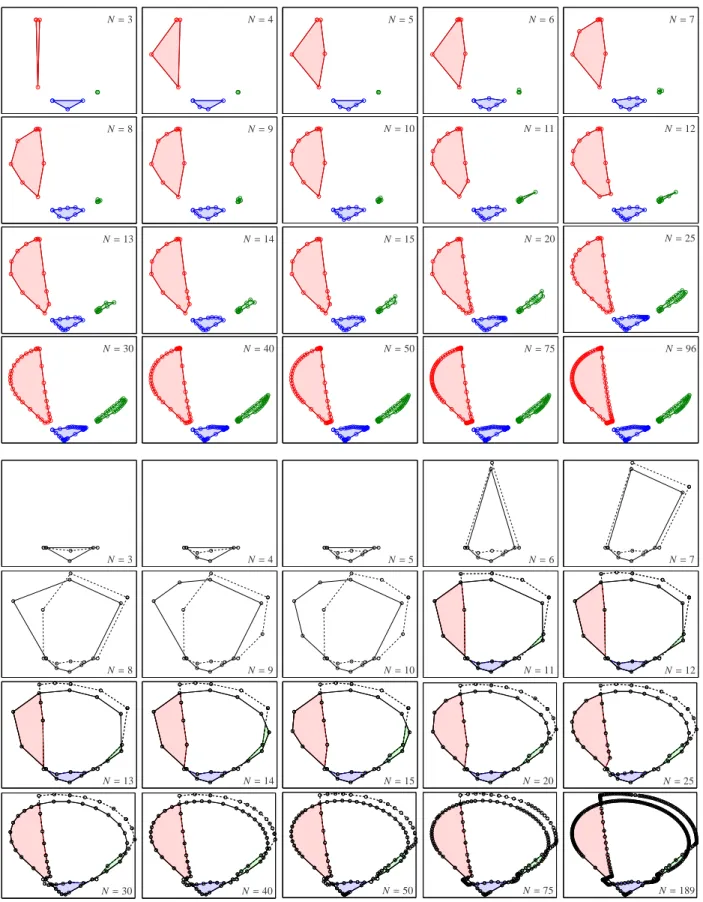
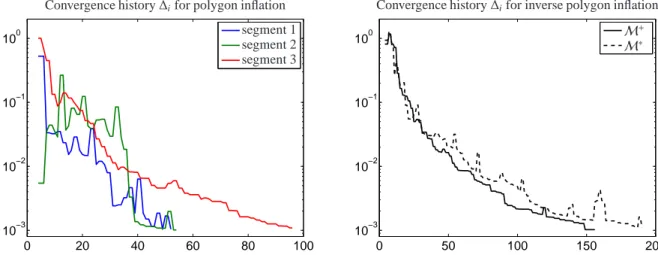
The polygon inflation algorithm [43] and its algo- rithmic variation of inverse polygon inflation [44] are adaptive methods for the computation of the AFS for three-component systems. The idea is to approximate the boundary of each segment of the AFS by sequences of step-by-step refined polygons. A combination of a local error estimation with a local strategy for the refine- ment of the polygon results in a very effective, adaptive approximation scheme. Various control parameters allow to steer the approximation process and its quality.

The polygon inflation method can be generalized to a

polyhedron inflation procedure in order to compute the AFS for four-component systems, see Section 7. We show some first examples in this work.

The geometric idea of the boundary approximation by inflating polygons is demonstrated in Figure 13. The shape of an Erlenmeyer flask is approximated in 2D by the polygon inflation method. Additionally the surface of a 3D Erlenmeyer flask is approximated by the polyhedron inflation algorithm. The surface of the polyhedron is a triangle mesh.

6.5.1. Steps of the polygon inflation algorithm

In this section the steps of polygon inflation method are explained. The inverse polygon inflation algorithm derives from the standard polygon inflation in a way that the setsM⁺andM^∗by Equations (7) and (8) are computed separately by inflating polygons. Then the AFS Mis computed by forming the intersectionM⁺∩ M^∗. Thus the costs for the inverse polygon inflation is less than twice that of the polygon inflation. For further details see [43, 44]. Next the single steps of polygon inflation are explained for the case of an AFS consisting of three separate segments.

Step 1: Computation of an initial factorization of D The first step of the polygon inflation method is to compute a nonnegative matrix factorization of D. Ac- cording to Equations (2) and (5) this allows to find three points in the (spectral) AFS; the planar coordinates of these points are the matrix elements of the second and third column of T . If the AFS consists of three sepa- rated segments, then each segment contains exactly one of these points. For each of these three points an associated polygon is inflated.

The following steps 2 and 3 are executed for each of the three points from Step 1 which are located in the three AFS segments.

13