A fast polygon inflation algorithm to compute the area of feasible solutions for three-component systems. II: Theoretical foundation, inverse polygon inflation and FAC-PACK implementation

A fast polygon inflation algorithm to compute the area of feasible solutions for three-component systems.

II: Theoretical foundation, inverse polygon inflation and FAC-PACK implementation

Mathias Sawall^a, Klaus Neymeyr^a,b

aUniversität Rostock, Institut für Mathematik, Ulmenstraße 69, 18057 Rostock, Germany

bLeibniz-Institut für Katalyse, Albert-Einstein-Straße 29a, 18059 Rostock, Germany

Abstract

The area of feasible solutions (AFS) of a multivariate curve resolution method is the continuum of feasible solutions under the given constraints. In the current paper the AFS is computed only on the condition of nonnegative solutions.

This work is a continuation of a paper (J. Chemometrics 28:106-116, 2013) on the polygon inflation algorithm for AFS computations. In this second part various properties of the AFS are analyzed. First, its boundedness is proved, which is a necessary condition for its numerical computation. Second, it is shown that the origin is never contained in the area of feasible solutions. This fact is the basis for the inverse polygon inflation algorithm, which allows to compute specific types of an AFS containing a hole.

The numerical computation of the AFS is a complicated and computationally expensive process. The construc- tion of proper objective functions for the AFS-optimization problem appears to be decisive. The paper contains a comparative analysis of two objective functions and describes the ideas of the newFAC-PACKtoolbox for MatLab. This freely available toolbox contains a numerical implementation of the polygon inflation and of the inverse polygon inflation algorithm.

Key words: factor analysis, pure component decomposition, nonnegative matrix factorization, area of feasible solutions, polygon inflation.

1. Introduction

The area of feasible solutions (AFS) represents the continuum of all solutions of multivariate curve reso- lution techniques under pre-given constraints. In this paper we consider the AFS only for nonnegativity con- straints on the spectral factor and on the concentration factor. The AFS allows to gain an overview on the pos- sible solutions from which an MCR method extracts one final solution by using soft and hard models. However, the reliability of the solution depends on the correctness of the models. A stable and precise numerical compu- tation of the AFS is a time-consuming process, which is made more difficult by noisy data.

The computation of the AFS for a two-component system goes back to Lawton and Sylvestre [1] in 1971.

Borgen and Kowalski [2] have extended AFS computa- tions to three-component systems in 1985. For further important contributions see [3, 4, 5, 6] and the refer-

ences therein. We use the term area of feasible solutions regardless of the dimension or number of components of the system since we understand the term not in the sense of a two-dimensional surface area but more in the sense of a region or territory.

In 2011 Golshan, Abdollahi and Maeder provided a new idea for the numerical approximation of the bound- ary of the AFS by a chain of equilateral triangles [7]. An alternative solution for such a numerical approximation of the AFS by a sequence of adaptively refined polygons has been suggested in the first part of this paper [8].

To our knowledge some topological properties of the AFS have never been analyzed. For instance, it is not clear that the AFS is (under some mild assumptions) a bounded set. Boundedness, however, is a necessary prerequisite for a successful numerical approximation.

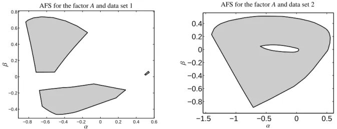
Often the AFS consists of three clearly separated sub- sets. It can also be a single topologically connected set with a hole; see Figure 1 for two typical areas of feasi-

... December 11, 2013

ble solutions. These different topologies require adapted computational strategies. All this justifies the following objectives:

1. analyze some theoretical properties of the Borgen and Kowalski approach to the AFS and their im- pact on properties of the AFS,

2. compare the two objective functions for the triangle-enclosure algorithm and the polygon infla- tion algorithm,

3. find approximation schemes which allow to ap- proximate the AFS for typical cases in which the AFS consists of three separated segments or only one segment with a hole,

4. present a fast and stable numerical method for the computation of such one-segment AFS,

5. show how the AFS can be reduced if additional in- formation on the factors is available.

The paper is organized as follows. In Section 2 some mathematical properties of the AFS are analyzed. Sec- tion 3 is devoted to a comparative analysis of two ob- jective functions which are key tools for the numerical AFS approximation. In Section 4 the new inverse poly- gon inflation scheme, which allows to compute an AFS with a hole, is introduced. The inverse polygon infla- tion algorithm is a central part of the newFAC-PACK toolbox in MatLabfor AFS computations. In Section 5 techniques are presented which allow to reduce an AFS by means of additional information on the factors. All this is accompanied by various numerical examples in sections 3, 4 and 5.

1.1. Data sets

Within this paper the algorithms and new concepts are tested for the three data sets:

1. Rhodium catalyzed hydroformylation, see [9, 8].

A number of k=1045 FT-IR spectra with n=664 spectral channels is used. There are s=3 indepen- dent components namely the olefin, the acyl com- plex and the hydrido complex. The AFS is shown in Figure 1 (left) and in Figure 6.

2. Formation of hafnacyclopentene, see [10, 11, 12].

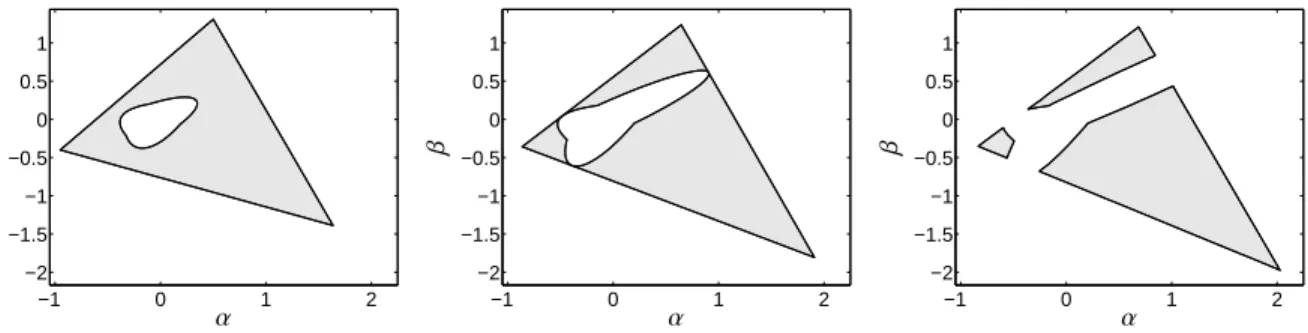
A number of k=500 UV/Vis spectra with n=381 spectral channels is given. The AFS for this system with s = 3 independent components is shown in Figures 1 (right) and 7.

3. ButiPhane ligands and hydrogenation activity, see [13]. A number of k=82 UV/Vis spectra with n= 1951 channels is given. The AFS for this system with s = 2 independent components is shown in Figure 3.

The collection of spectra for these three reaction sys- tems are shown together with the concentrations profiles and spectra of the pure components at the end of this pa- per in Figures 8–10. For more details on these problems see [9], [11] and [13].

2. On the AFS

The Borgen and Kowalski [2] approach to the AFS for three-component systems together with further ref- erences and explanations has been introduced in the first part [8] of this paper in Section 2.2. Next only those equations are compiled which are essential for this pa- per.

The starting point is a k×n spectral data matrix D whose nonnegative factorization CA is desired. The k× s concentration matrix C contains the concentra- tion profiles of the s components in its columns, and the s×n spectral factor A contains the associated s pure- component spectra in its rows. Usually, a given D has an infinite number (or continuum) of nonnegative factor- izations. The AFS is a low dimensional representation of these solutions. If D has the rank s, then the truncated rank-s singular value decomposition reads D = U ˜˜ΣV˜ with ˜U ∈R^k×s, ˜Σ∈R^s×sand ˜V ∈R^n×s. This allows to set C=U ˜˜ΣT⁻¹and A=T ˜V^Twhere T is an s×s regu- lar matrix and D=U ˜˜ΣT⁻¹T ˜V^T. If D contains perturbed spectral data, then the rank of D is usually larger than s and the upper relations hold in an approximate form.

The AFS for an s-component system is a subset of theR^s−1with the form

M={t∈R^1×s−1: exists invertible T ∈R^s×s, T (1,:)=(1,t), U ˜˜ΣT⁻¹≥0 and T ˜V^T ≥0}. (1) For a three-component system this simply reads

M={(α, β)∈R²: det(T ),0, C,A≥0}

with C=U ˜˜ΣT⁻¹, A=T ˜V^T and

T =













1 α β

1 s₁₁ s₁₂ 1 s₂₁ s₂₂













. (2)

2.1. Mathematical foundation

The definition ofMin (1) implies that the rows a of a feasible factor A can be presented by linear combina- tions of the rows of ˜V^T in the form

a=(1,t)·V˜^T. (3) 2

−0.8 −0.6 −0.4 −0.2 0 0.2 0.4 0.6

−0.4

−0.2 0 0.2 0.4 0.6 0.8

α

β

AFS for the factor A and data set 1

−1.5 −1 −0.5 0 0.5

−0.8

−0.6

−0.4

−0.2 0 0.2 0.4

α

β

AFS for the factor A and data set 2

Figure 1: Typical areas of feasible solutions. Left: Three separated segments forming the AFS (Data set 1: hydroformylation process). Right: The AFS is a connected set with a hole (Data set 2: formation of hafnacyclopentene).

The fixed 1 in the row vector (1,t) guarantees that any spectrum has a contribution from the first right singular vector. This property is by no means evident and has to be proved. Theorem 2.2 shows that the AFS represen- tation (1) is valid if and only if D^TD is an irreducible matrix. For such matrices Theorem 2.4 shows thatMis a bounded set. Boundedness is a necessary prerequisite for the numerical techniques in [7, 8] to compute the AFS. To our knowledge no proof on the boundedness has been given so far.

The central results of this section are Theorems 2.2 and 2.4. In these theorems rank(D)=s is assumed with s≥2. The results do not necessarily hold for perturbed data and if s is smaller than rank(D). Some implications of these theorems are summarized at the end of this sec- tion.

Definition 2.1. Let P be an n×n permutation matrix, i.e. P is a column permutation of the identity matrix.

An n×n matrix H with n≥2 is called reducible, if a permutation matrix P exists so that

PHP^T= H1,1 H1,2

0 H2,2

! .

Therein H1,1is an m×m submatrix and H1,2is an m× (n−m) submatrix with 1≤m<n. If such a permutation matrix P does not exist, then H is called an irreducible matrix.

The next theorem proves that the Borgen and Kowal- ski approach (with 1s in the first column of T ) is justi- fied. Further, the result is used in Theorem 2.4 on the boundedness of the AFS.

Theorem 2.2. Let D ∈ R^k×n be a nonnegative matrix with rank(D)=s which has no zero column. Further let UΣV^T be a singular value decomposition of D and let V be the submatrix of V formed by its first s columns.˜

There exists no row vector t∈R^1×s−1\ {0}with (0,t)·V˜^T ≥0 (4) (in words: any linear combination of the columns 2, . . . ,s of ˜V has negative components) if and only if D^TD is an irreducible matrix.

Proof. First let D^TD be irreducible. The Perron- Frobenius-theorem [14] guarantees that the first right singular vector V(:,1) is a sign-constant vector without zero components. This means that either V(:,1) > 0 or V(:,1) < 0. If V(:,1) > 0 and assuming a vector t∈R^s−1\ {0}satisfying (4), then it holds that

(0,t)·V˜^T

| {z }

≥0 and,0

·V(:,˜ 1)

|{z}

>0

>0.

This is a contradiction to the orthogonality of ˜V since its first column ˜V(:,1) is orthogonal to all the remain- ing columns ˜V(:,2 : s). For the case V(:,1) < 0 the arguments are almost the same.

In order to prove the opposite direction by contrapo- sition, let D^TD be a reducible matrix. According to Def- inition 2.1 there is a permutation matrix P so that

PD^TDP^T = D1 0 0 D2

! .

The right upper block is also a zero block since PD^TDP^Tis a symmetric matrix.

3

By assumption D has no zero-columns so that all dia- gonal elements of D^TD are nonzero; i.e., d_k^Tdk , 0 where d_kis the k-th column of D. Therefore PD^TDP^T has no zero-columns so that D₁and D₂are nonzero and nonnegative matrices. Without loss of generality D1and D2can be assumed to be irreducible matrices; otherwise the argumentation is applied to proper irreducible sub- matrices.

Letλ1 andλ2be the eigenvalues of D1resp. D2with the largest modulus. The Perron-Frobenius theorem guarantees that λ1 and λ2 are (by irreducibility) sim- ple and positive eigenvalues. The associated normal- ized eigenvectors u1 and u2 are component-wise pos- itive vectors. These eigenvectors are among the right singular vectors of D so that for proper indexes i1,i2

P ˜V(:,i1)= ±u₁ 0

!

, P ˜V(:,i2)= 0

±u₂

!

. (5)

Therein ± expresses that the orientation of a singu- lar vector is not uniquely determined. Without loss of generality let i₂ , 1 (otherwise i₁ , 1). Then let (0,t) :=±e^T_i

2where e_i2is the standard basis column vec- tor whose i₂-th component equals 1 and all other com- ponents are 0. From (5) one gets

P ˜V(±ei₂)= 0 u2

!

≥0.

Transposition of this equation and right multiplication by P results in

±e^T_i

2

V˜^T P^TP

|{z}

I

=(0,u^T₂) P≥0.

Together with (4) this completes the proof.

Corollary 2.3. Let D^Tsatisfy the assumptions of Theo- rem 2.2. Then noυ∈R^s−1exists with

U ˜˜Σ 0 υ

!

≥0 if and only if DD^Tis irreducible.

Proof. From D^T = V ˜˜ΣU˜^T and non-existence of t with (0,t) ˜U^T ≥0 if and only if DD^T is irreducible one gets the non-existence of t with (0,t) ˜ΣU˜^T ≥0. Transposition of the last inequality proves the proposition.

The matrix D^TD can be assumed to be irreducible for spectroscopic applications. Otherwise, the series of spectra decomposes into apparently separated or non- coupled subblocks. A trivial example of a reducible matrix is the 3-by-3 identity matrix D = I3 so that

D^TD = I3 for which T is not necessarily in the form (2) (since V =T =T⁻¹=C=A=I3 ≥0 is a feasible solution).

An important consequence of Theorem 2.2 is that the AFS is a bounded set. The AFSMis a subset of

M⁺ ={t∈R^1×s−1: (1,t) ˜V^T ≥0}, (6) which is closely related to FIRPOL in [2, 3]. The set M⁺ stands for the nonnegativity of the spectral factor A only, andM⁺ is the intersection of the n half-spaces

{t∈R^1×s−1: t ˜V(i,2 : s)^T ≥ −V(i,˜ 1)}, i=1, . . . ,n.

(7) The next theorem shows thatMandM⁺ are bounded sets for irreducible D^TD.

Theorem 2.4. Let D satisfy the assumptions of Theorem 2.2. ThenM⁺ by (6) andMare bounded if and only if D^TD is an irreducible matrix.

Proof. SinceM⁺ is an intersection of the half-spaces (7), boundedness of M⁺ means that there is no t ∈ R^1×s−1so that according to (6)

(1, γt) ˜V^T ≥0 (8)

for all γ ≥ 0 (otherwiseM⁺ would be unbounded in the direction t).

Inequality (8) can be rewritten as γt ˜V(:,2 : s)^T ≥0≥ −V(:,˜ 1).

The null vector has been inserted in this chain of in- equalities which is justified because ˜V(:,1) is a nonneg- ative vector. Hence boundedness means that there is no t ∈R^1×s−1so that t ˜V(:,2 : s)^T ≥0. Equivalently, there is no t so that (0,t) ˜V ≥0 and thus D^TD is irreducible due to Theorem 2.2. This proves the assertion forM⁺. AsMis a subset ofM⁺ the proof is completed.

With few additional assumptions one can show that the setMdoes not include the origin (i.e. the zero vec- tor).

Theorem 2.5. Let D ∈ R^k×s be a nonnegative rank-s matrix so that D^TD and DD^T are irreducible matrices and that a factorization D=CA with nonnegative fac- tors exists. Then 0<M.

Further, the first left singular vector ˜U(:,1) is not the concentration profile of a pure component and the first right ˜V(:,1) is not the spectrum of one of the pure com- ponents.

4

Proof. Let D = CA be a factorization with 0 ≤ C ∈ R^k×sand 0≤A∈R^s×n. According to (1) the first row of A equals A(1,:)=(1,t) ˜V^Tfor some t∈ M. The concen- tration profile of the second component is C(:,2)=U ˜˜Συ forυ∈R^s. Corollary 2.3 proves thatυ₁,0.

Thus (1,t) is the first row of T andυis the second column of T⁻¹. From

0=I1,2=(T T⁻¹)1,2=(1,t)·υ

one derives 0,υ1 =−t·υ(2 : s,1). Thus neither t nor υ(2 : s,1) are null vectors. So 0<Mand ˜V(:,1) is not equal to a pure component spectrum. Applying the ar- guments to D^T shows that ˜U(:,1) is not a concentration profile of a pure component.

3. Objective functions

The numerical computation of the AFS for s=3 and even larger s is a complicated and computationally ex- pensive process. There is no closed-form-representation of the AFS which could simply be drawn by the evalu- ation of a function. Noisy data makes the computation of the AFS even more difficult.

For three-component systems Borgen and Kowalski [2] as well as Rajkó and István [3] presented for noisy- free data a geometric approach to the construction of the AFS. A direct numerical approximation of the AFS for three-component systems and noisy data can be com- puted by means of the triangle-enclosing algorithm [7]

and the polygon inflation algorithm [8]. These iterations aim at an approximate computation of the boundary of the AFS. The central process behind these algorithms is a routine which decides whether a certain point (α, β) is contained inM. Such points are called valid. Points exterior toMare non-valid points.

The algorithms in [7] and [8] make use of different objective functions. Next these objective functions are compared for general s-component systems. The first objective function requires a more expensive computa- tional process compared to the second function. The two algorithms give the same results for nonnegative data. In case of noisy data the resulting AFS approx- imations may slightly differ.

3.1. The AFS for s-component systems

According to (1) and (2) the problem for an s- component system is to find regular matrices

T =



















1 t1 . . . ts−1

1 ... 1

S



















∈R^s×s (9)

with a row vector t =(t1, . . . ,ts−1)∈ R^1×s−1and a sub- matrix S ∈ R(s−1)×(s−1)in a way that C =U ˜˜ΣT⁻¹ and A =T ˜V^T are nonnegative matrices. In order to decide whether t is valid (t ∈ M) or non-valid (t<M) one has to solve an optimization problem. The solution is either a proper submatrix S or its non-existence can be stated.

We call this process the AFS-decision over (t,S ).

3.2. Thessqapproach

The AFS-decision over (t,S ) in [4, 5, 7] is based on ssq:R^s−1×R(s−1)×(s−1)→R, (t,S )7→ kD−C+A+k²_F with

C+=max( ˜U ˜ΣT⁻¹,0), A+=max(T ˜V^T,0) and T given by (9). Furtherk · kFdenotes the Frobenius norm [15].

By usingssqthe AFSMis M=

t∈ M⁺ : min

S∈R(s−1)×(s−1)ssq(t,S )≤ǫ

(10) withǫ =0. For practical computations in presence of rounding errors one can useǫ =10⁻¹². The minimiza- tion problem in [7] has been solved by the Nelder-Mead simplex minimization (MatLabroutinefminsearch).

This approach is summarized as follows:

Objective function 1. The AFS-decision over (t,S ) re- sults in a valid t, i.e. t ∈ M, if the minimization of the objective functionssqyields 0 up to rounding errors.

3.3. Alternative approach to the AFS-decision

Next an alternative minimization problem is dis- cussed with a much smaller number of squares. A first rapid test on the validity of t∈ Mcan result in an addi- tional acceleration of the computational process.

We start with this rapid test for a given t. Nonnega- tivity of T ˜V^Timplies that

−t·V(i,2 : s)^T ≤V(i,1), i=1, . . . ,n. (11) This test does not require the computation of S in (9) so that the computational costs for checking (11) are negligible.

If a certain row vector t has passed the test (11), then we consider the function

f :R^s−1×R(s−1)×(s−1)→Rks+n(s−1)+1, (12) (t,S )7→













min(0,Cil) min(0,Aℓj) kI_s−T⁺Tk²_F













ks components n(s−1) components 1 component.

5

min

(1, α, β)·V˜^T

≥0

(α, β)<M minSkf (t,S )k²₂≤ǫ

(α, β)<M (α, β)∈ M no yes

yes no

Figure 2: Decision tree for objective function 2. The dashed ellipse expresses some uncertainty as the numerical minimization concerning S may fail, cf. Section 3.5.

The first ks components of f are either equal to 0 or the negative components of C ∈ R^k×s. The following n(s−1) components of f are either equal to 0 or the negative components of A∈R^s×n; the first row of A has not to be checked on negative components due to the test (11). The last component of f aims at avoiding a rank-deficient matrix T with rank(T )<s.

The least-squares minimization of f includes a num- ber of ks+n(s−1)+1 squares. Since s is a fixed small number and k as well as n are potentially large the total costs for minimizing (12) increases asO(k+n) wherein Ois the Landau symbol. In contrast to this, thessqap- proach is more expensive withO(kn). For the numerical minimization of kf (t,S )k²₂ a code for nonlinear least- squares minimization can be applied likelsqnonlinin MatLab. For ourFAC-PACKimplementation we use the FORTRAN code NL2SOL [16].

With (12) this allows to define the area of feasible solutions as follows

M=

t∈ M⁺ : min

S∈R(s−1)×(s−1)kf (t,S )k²₂≤ǫ

.

Theoreticallyǫ =0 but we useǫ =10⁻¹⁰ for practical computations.

Objective function 2. The AFS-decision over (t,S ) re- sults in a valid t, i.e. t ∈ M, if the test (11) is passed and the minimization of the objective function f results in 0 up to rounding errors. The decision tree is shown in Fig. 2.

3.4. Negative components

Noisy spectral data or negative components of the spectral data matrix D due to some data preprocessing does not always allow to find nonnegative matrix factors

C and A. A proper treatment of small negative compo- nents of these matrices appears to be crucial for a suc- cessful construction of the AFS. The approaches from Sections 3.2 and 3.3 treat such negative components dif- ferently.

Let us first discuss the limit case of

min_S∈R(s−1)×(s−1) f (t,S ) = f (t,S^∗) = 0. Then by

definition of f , see Equation (12), it is guaranteed that C and A are nonnegative matrices. Thus

max(C,0)·max(A,0)=C·A=D.

This implies thatssq(t,S^∗)=0. It is not clear that the other case of a vanishingssqof D−C+A+implies that f also vanishes. To show this, the reconstruction D = C+A+with the truncated matrices C+and A+must imply C−=0 and A−=0. It is not clear if such properties can be proved. But as C+ and A+are feasible nonnegative factors they are in any case represented by the AFS.

Here we accept the factors C and A if the relative neg- ative portion in the columns of C and the rows of A is bounded as follows

minjCji

maxj|Cji|≥ −ε, minjAi j

maxj|Ai j| ≥ −ε

for i = 1, . . . ,3. The parameterε, see Section 3.3, is taken asε=10⁻¹²for model problems without pertur- bations.

Similarly the first rapid test (11) is reformulated as V_i1+t₁V_i2+· · ·+ts−1V_is

k(1, t)·V^Tk_∞ ≥ −ε, i=1, . . . ,n.

Thereink · k_∞is the maximum norm, i.e. the maximum of the absolute values of the components.

Further, the first ks components of f are taken as min(0,Cil/kC(:,l)k_∞+ε)

and the following n(s−1) components are similarly min(0,Aℓj/kA(ℓ,:)k_∞+ε).

3.5. Reliability of the numerical optimization

The AFS-decision for a vector t ∈ R^s−1is a numer- ically expensive and potentially instable process since for the given t a proper S is to be computed by solving an optimization problem. This numerical computation may fail. In particular such problems are to be expected if only a poor initial approximation for S is available at the start of the optimization procedure.

However, for two-component systems the situation is very simple, see Section 3.6. For s≥3 the decision tree 6

−0.15 −0.1 −0.05 0.2

0.3 0.4 0.5 0.6

α

β M

Figure 3: AFS for a two component system for the ButiPhane data.

shown in Figure 2 applies. The rapid test on nonnegativ- ity by inequality (11) appears to be non-critical. Further, any decision t ∈ Mcan be trusted as the optimization process has found a solution. A decision t< Mdue to minSkf (t,S )k²₂ > ǫmay not be trusted as, e.g., the op- timization procedure may have got stuck in a local and non-global minimum. To reduce the risk of such mis- classifications we always take special care to generate good initial values for S . Such initial matrices can be computed by local averaging final and trusted matrices S on points in a close neighborhood of t.

3.6. The AFS for two-component system

For a two-component system the matrix T is simply given by

T = 1 α

1 β

! .

If we ignore noise and letε=0, then using the objective function 2 results in

(α, β)∈[a,b]×[c,d] or (β, α)∈[a,b]×[c,d]

with

a=− min

i: V(i,2)>0

Vi1

V_i2, b=min

i

Ui2σ2

U_i1σ1

, c=max

i

Ui2σ2

Ui1σ1

, d=− max

i: V(i,2)<0

Vi1

Vi2

. Thus the AFS for a two-component system consists of two real intervals. These two intervals are usually rep- resented by the sides of a rectangle, cf. [5]. A point within this rectangle allows a simultaneous representa- tion of the AFS for the spectral and for the concentration factor (which is fundamentally different from the AFS for three-component systems where either the AFS for the spectral factor or the AFS for the concentration fac- tor is represented in 2D). It is also clear that b<0<c and that eitherα < 0 andβ >0 or alternativelyα >0 andβ < 0. All this is consistent with 0< Mwhich is

dimension objective fct. 1 objective fct. 2

k n time [s] time [s]

75 50 9.15 1.23

150 100 33.31 1.68

300 200 133.04 2.82

450 300 271.95 3.47

750 500 803.86 5.45

1500 1000 3773.88 11.26

Table 1: Total computing times for programs using the two objective functions for the model from [8]. In each of these cases the AFSMC

and the AFSMAare computed.

proved in Theorem 2.5. In case of noisy data, the AFS is still a rectangle. Then the scalars a, b, c and d can be computed numerically by using the bisection method.

For instance a and d are the minimal or maximal value ofαso that

(1, α)V^T k(1, α)V^Tk∞

≥ −ǫ

and b, c are computed analogously by using linear com- binations of UΣ. Figure 3 shows the two-dimensional AFS for the ButiPhane data set, which is data set 3 in Section 1.1.

3.7. Computational costs

Next a direct comparison of the computational costs is given for the two objective functions presented above.

First we consider a three-component model problem and second we use FT-IR spectral data from the hydro- formylation process. The two objective functions are each applied within the polygon inflation algorithm in order to present in detail the effect of the choice of the objective functions.

3.7.1. A model problem

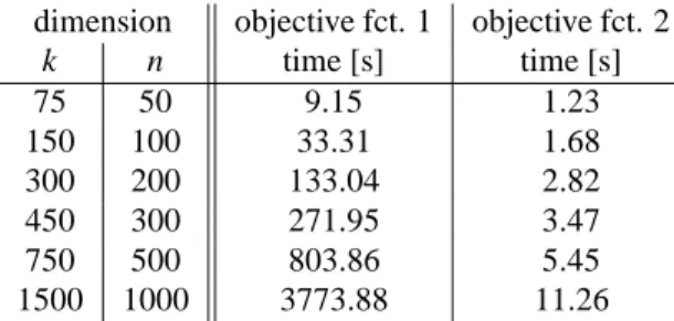
The three-component model problem is taken from part I of this paper; see Section 4.1 in [8]. Here we consider a series of different values for k, the number of spectra, and n, the number of spectral channels, see Table 1. The last two columns of Table 1 give the total computational times for programs using the objective functions 1 and 2. For these computations the parame- tersε=10⁻¹² andεb =δ= 10⁻³ have been used; see Part I for the explanation ofεbandδ.

Figure 4 shows the computation time against kn in a log-log plot. The computational costs for the first ob- jective function increases withO(kn). The second ob- jective function results in a much faster method. The numerical data are consistent with costs increasing as O(k+n).

7

10⁴ 10⁵ 10⁶ 10⁰

10¹ 10² 10³

Computing time

time[s]

dimension kn

objective fct. 1 objective fct. 2

Figure 4: Bilogarithmic plot of the data from Table 1.

AFS objective fct. 1 objective fct. 2 time [s] time [s]

M_C 998.32 4.58

M_A 862.33 4.39

Table 2: Computing times for the two objective functions for the Rhodium catalyzed hydroformylation. The times forMCandMA

are tabulated separately.

3.7.2. Rhodium catalyzed hydroformylation

Next we consider the Rhodium catalyzed hydro- formylation as given by the data set 1 in Section 1.1.

Now the parameters areε=−0.01 andε_b =δ=10⁻³. The computational times in Table 2 confirm that the sec- ond objective function results in a much faster method.

The resulting areas of feasible solutions are almost iden- tical if the same valueεbfor the boundary precision is used. The associated Hausdorffdistances for the three segments of the AFS are given in Table 1 of [8].

4. Inverse polygon inflation for an AFS with a hole As shown in Section 2 the AFS is a bounded set which does not include the origin. A challenging ques- tion is: What is the number of isolated segments an AFS may consist of?

For s = 2-component systems the AFS consists of p=2 separated intervals which are taken as the sides of a rectangular for its presentation; see [1, 5] or Section 3.6. For s = 3-component systems experimental data and model data show that a number of p = 1, p = 3 or even p = 6 segments may occur. We plan to give a mathematical proof that an AFS with two segments cannot occur in a forthcoming publication. A further

interesting question is to show that the number of AFS segments ofM_AandM_Ccoincide.

It is well known that the AFS for three-component systems may consist of only one segment and that this segment can contain a hole, which surrounds the origin.

Next we describe a variation of the polygon inflation al- gorithm which can be used to compute such AFS with a hole or an AFS with more than three isolated segments.

4.1. Inverse polygon inflation

If for a three-component systems (s = 3) the en- tire AFS consists of one segment with a hole, then the triangle-enclosure algorithm [7] and the polygon infla- tion algorithm are to be modified properly. For the triangle-enclosure algorithm two runs are necessary in order to cover the interior and the exterior boundary curve by sequences of triangles.

For the polygon inflation algorithm the exterior poly- gon and the interior polygon are to be treated differently but the geometric concept of inflation polygon is in each of these cases the same. Only the objective functions are changed.

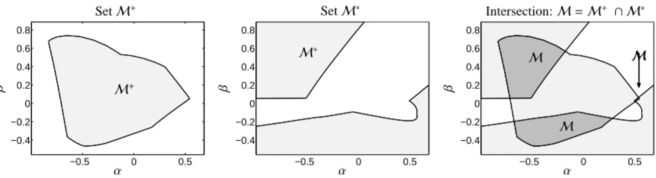
First, the computational effort to compute the exte- rior polygon is very small since only (1,t) ˜V^T ≥ 0 is to be tested according to Equation (6), cf. FIRPOL in [2]. This exterior polygon is just the boundary of the set M⁺ defined in (6). The remaining conditions on t to be a valid vector, i.e. t∈ M, are used to define a further set

M^∗ ={t∈R^s−1: min

S kf (t,S )k²₂=0} (13) whose inner boundary is computed by the standard polygon inflation algorithm. For t ∈ M^∗ the defini- tion of M^∗ guarantees that T is regular, C ≥ 0 and A(2 : 3,:)≥0. The intersection ofM⁺ andM^∗, which combines the conditions, results in the AFS

M=M⁺ ∩ M^∗. (14) In order to avoid any misinterpretation we mention that M^∗ is very different to INNPOL as used in [2, 3].

The algorithm to compute a polygon which approxi- mates the boundary ofM⁺ uses an objective function which guarantees (7) to hold. The starting point is the origin which is always inM⁺. The polygon inflation starts with a triangle enclosing the origin and whose ver- tices are located on the boundary ofM⁺.

After this the interior boundary ofM^∗ is computed by using the objective function (12). Therefore the com- plementR²\ M^∗ is approximated from the interior of this set. The starting point is, once again, the origin since Theorem 2.5 guarantees that (0,0) < M^∗ . The 8

−1 0 1 2

−2

−1.5

−1

−0.5 0 0.5 1

α

β

−1 0 1 2

−2

−1.5

−1

−0.5 0 0.5 1

α

β

−1 0 1 2

−2

−1.5

−1

−0.5 0 0.5 1

α

β

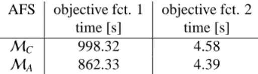
Figure 5: Breaking-up of the AFSMAfrom one to three segments for the Example 4.1 withω1 =1.5. Left: Only one segment with a hole for ω2 =0.5. Center: The hole touches each side of the outer triangle forω2 =0.26787. Right: Forω2 =0.2 the AFS is broken into three clearly separated segments.

usage of the complement is the reason why we call the algorithm an inverse polygon inflation. The computa- tion of the hole of the AFS by applying the polygon in- flation toR²\ M^∗ has the advantage that only few lines of program code are to be adapted. Further, the relevant regions of the two setsM⁺ andM^∗ can be computed in a stable way.

IfFAC-PACKuses the standard polygon inflation al- gorithm and finds an AFS segment which has a nonzero intersection with at least three quadrants of the Carte- sian coordinate system, then the algorithm automati- cally switches to the inverse polygon inflation. Thus a one-segment AFS is automatically computed by inverse polygon inflation.

4.2. FAC-PACKsoftware for AFS computations The polygon inflation algorithm and the inverse poly- gon inflation algorithm are implemented in the software toolbox FAC-PACK for Matlab [17]. FAC-PACK contains a graphical user interface from which the spec- tral data can be loaded, a singular value decomposition and an initial nonnegative matrix factorization (NMF) can be computed. This NMF is the starting point for the computation of the AFS.FAC-PACKallows to display the spectral and concentration factors which are asso- ciated with any points of the AFS. Further, one or even two components can be locked and the resulting reduced AFS is shown.

TheFAC-PACKhomepage containing the software and a tutorial can be accessed at

http://www.math.uni-rostock.de/facpack/

4.3. Weakly separated segments of the AFS

If the segments of an AFS are only weakly separated (in a sense that the polygon inflation algorithm tends to glue separated segments of the AFS to a joint segment;

see the AFS in the mid of Figure 5), then the numerical

computation ofM⁺ andM^∗, which is followed by their intersection, is a stable and favorable way to construct M. The inverse polygon inflation procedure can even be applied to general situations with well separated seg- ments - a situation we have often found for FT-IR spec- tral data. However, the computational procedure for the inverse polygon inflation is somewhat more expensive compared to the direct computation of the three sepa- rated segments.

4.4. AFS dynamics showing the separation process In order to study the possible shapes of an AFS we il- lustrate the transition of the AFS from one topologically connected segment to an AFS formed by three segments for a three-component model problem. In this separa- tion process three segments which pairwise touch in one point split up to three clearly separated segments. The case of only two separated segments is not observed; we will give a mathematical proof on this in a forthcoming paper. The model problem depends on two real param- etersω1andω2.

Example 4.1. Let D∈R^3×3be the nonnegative matrix

D=













1 0 0

0 1 0

0 0 1











 +ω1













0 0 0

1 0 0

1 1 0











 +ω2













1 1 1

0 1 1

0 0 1











 .

Nonnegative factorizations D =CA and the AFS M_A are to be computed.

For our computations the parameter ω1 is fixed to ω1 =1.5 andω2is used as a variable. Figure 5 shows that the AFS for ω2 = 0.5 is one topologically con- nected set. For ω₂ = 0.26787 the AFS consists of three segments which pairwise touch in one point. For ω₂=0.2 one gets three clearly separated segments.

Various numerical experiments indicate that the AFS MA for three-component systems is either formed by 9

−0.5 0 0.5

−0.4

−0.2 0 0.2 0.4 0.6 0.8

SetM⁺

α

β M⁺

−0.5 0 0.5

−0.4

−0.2 0 0.2 0.4 0.6 0.8

SetM^∗

α

β

M^∗

−0.5 0 0.5

−0.4

−0.2 0 0.2 0.4 0.6 0.8

Intersection:M=M⁺ ∩ M^∗

α

β

M

M MMM

Figure 6: Results of inverse polygon inflation for the hydroformylation data set 1 from Section 1.1. Left: The boundary ofM⁺ according to Eq. (6) is similar to FIRPOL [2]. Center: The setM^∗ according to (13) is shown in the sameα, β-window for whichM⁺is computed. This avoids useless computations sinceMis a subset ofM⁺. Right: The AFSMis the intersectionM ∩ M^∗.

one topologically connected segment or by three iso- lated segments. The same holds for the AFSMC. Spe- cially constructed matrices D may have much more iso- lated segments.

4.5. The AFS for spectroscopic data

1. Data set 1 - the Rhodium catalyzed hydroformy- lation: The reference to this FT-IR spectroscopic data is given in Section 1.1. The spectral AFS for this problem is computed by inverse polygon in- flation. Figure 6 shows the setsM⁺ (left),M^∗ (center) and their intersectionM, see also Figure 1.

2. Data set 2 - formation of hafnacyclopentene: The reference to this UV/Vis data set is given in Section 1.1. The AFSM=M_Ais shown in Figure 1 (right plot) and is one topologically connected set with a hole, which contains the origin. This relatively large AFS imposes only weak restrictions on the factor A since the associated spectra are nowhere equal to zero. All this allows a wide range of fea- sible transformation making the AFS large.

4.6. How to compute line-shaped segments of the AFS An isolated segment of the AFS is most often either a set whose (mathematical surface) area is larger than zero or it is a single point. In some cases an isolated sub- set of the AFS appears to be a straight-line segment. In absence of rounding errors and perturbations its surface area equals zero; for slightly perturbed data such a seg- ment practically is a long and narrow band. The polygon inflation method needs some algorithmic enhancement in order to compute such straight-line segments.

InFAC-PACKwe use an angle-search method for approximating such AFS segments. The starting point is a feasible coordinate x = (α, β) as computed by the

NMF. Together with a small radius parameter r the func- tion

gr,x(ϕ)=x+r sin(ϕ) cos(ϕ)

!

is considered in order to compute a feasible angleϕso that gr,x(ϕ) ∈ M. The numerical minimization of the objective function (12) is executed only if the rapid test (11) is passed. The initial x might be one of the end- points of the line segment or between them. In the latter case and ifϕrepresents a feasible direction, then also ϕ−πstands for a feasible direction. For these two op- positely oriented direction maximal values rland rrare computed by the bisection method so that the desired line segment equals the unionLl∪ Lrwith

L_l= (

x+r sin(ϕ−π) cos(ϕ−π)

!

with r∈[0,r_l] )

, L_r=

(

x+r sin(ϕ) cos(ϕ)

!

with r∈[0,r_r] )

.

5. How to use additional information on the factors Nonnegativity of the factors is the only restriction which underlies the construction of the AFS. However, sometimes additional information on the factors is avail- able. This information may consist of the knowledge on certain pure-component spectra or concentration pro- files. Alternatively, some isolated peaks within a spec- trum may be known. In a recent work Beyramysoltana, Rajkó and Abdollahi [18] have shown a correlation of known factors for three-component systems in the spec- tral space with lines in the concentration space and vice versa. Comparable results for two-component systems are analyzed by Rajkó [19].

10

The software toolboxFAC-PACKallows to lock cer- tain spectra or concentration profiles and then to com- pute the reduced and smaller AFS for the remaining components [17]. In this section we focus on the mu- tual effect of reducing the AFS for A on the AFS for C and vice versa.

Further sources of additional information on the fac- tors might be window factor analysis (WFA) techniques or the evolving factor analysis [20, 21]. In this con- text the theorems of Manne [22] might help to extract concentration profiles of certain components. The im- plementation of such local rank information as a part ofFAC-PACKis a point for the future work. One can also use constraints like unimodality or the proximity of a spectrum in the AFS to a pre-given spectrum in or- der to reduce the ambiguity. However, in this paper we concentrate on computing the AFS under nonnegativity constraints and we do not want to dilute this approach by introducing too much adscititious information.

5.1. Three-component systems

To discuss a typical and concrete problem we as- sume that the first spectrum A(1,:) of a three-component system is known. As shown in [12] by coupling and complementarity theorems the knowledge of this spec- trum imposes an affine-linear constraint on the asso- ciated column C(:,1) and further linear constraints on the remaining columns C(:,2 : s). So the knowledge of A(1,:) considerably reduces the original AFS for A.

Additionally, the points representing the complemen- tary concentration profiles C(:,2 : 3) are restricted to a straight line through the AFS for C. The details are as follows: A known spectrum A(1,:) is represented by the coordinates (t2/t1, t3/t1) in the spectral AFS MA with t=(t1,t2,t3)=A(1,:)·V(:,1 : s). Theorem 4.2 in [12]

shows, that the concentration profiles C(:,2) and C(:,3) are elements of the subspace

{UΣy : t·y=0}={U ˜y : t·Σ⁻¹·˜y=0}.

Together with the required scaling ˜y₁ = 1 and using (α, β) as coordinates inM_Cthis subspace reads

L={(α, β) : t·Σ⁻¹·(1, α, β)^T=0}

= (

(α, β) : t2

σ2

α+ t3

σ3

β=−t1

σ1

) .

Thus L is a straight line through M_C and the (α, β)- representatives of the complementary concentration profiles C(:,2) and C(:,3) are located on this line.

This reduction process can be continued if a second spectrum A(3,:) is pre-given. For the concentration fac- tor C this means that points in the AFS which represent

the two concentration profiles C(:,1 : 2) are located on a further straight line. Together with the first straight line the intersection of these lines uniquely determines the second concentration profile C(:,2). This situation has explicitly been discussed in [12]; see there Theorem 4.2, Corollary 4.3 and Section 6.1. All these restrictions can be combined with any further information/constraints on C and A. However, if C(:,i) and A(i,:) for a certain i are pre-given simultaneously, then the whole problem can be reduced by this component.

5.2. Numerical example

Next we consider UV/Vis spectra for the formation of hafnacyclopentene given by data set 2 in Section 1.1;

see also Section 6.1 of [12]. For this three-component system the initial concentrations of the consecutive re- action X → Y → Z are cX(0) =0.01309 and cY(0) = cZ(0) = 0. The last spectrum of this series is a good approximation of the spectrum of the reaction product Z as the reaction is more or less completed. Together with the first spectrum two pure component spectra are available.

The AFS and its reductions are presented in three steps:

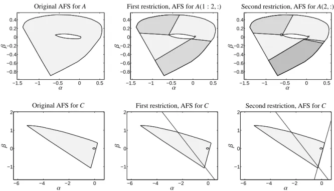
1. The initial areas of feasible solutions for C and A are shown in Figure 7 in the left column. No ad- scititious information has been used for the AFS computation.

2. If A(:,1) for the reactant X is given, then the ini- tial AFS can be reduced to two smaller segments, which are shown in Figure 7 in a darker gray. The bold straight line in the AFS for C in Figure 7 (sec- ond row and second column) covers the comple- mentary concentration profiles C(:,2 : 3).

3. If finally the spectrum A(:,3) for Z is also given, then the resulting AFS is reduced to the right lower AFS segment which is shown in Figure 7 by the darkest gray. A second straight line is added to the AFS for C. Figure 7 (second row and third column) shows this by another bold line. The in- tersection of the two lines uniquely determines the concentration profile C(:,2).

5.3. Remark on the AFS for multi-component systems The AFS for a system with s independent compo- nents is a bounded set in the s−1-dimensional space according to Equation (9). Additional information on the factors can be applied to such a higher-dimensional AFS in a way which is comparable to the techniques explained above.

11

−1.5 −1 −0.5 0 0.5

−0.8

−0.6

−0.4

−0.2 0 0.2 0.4

Original AFS for A

α

β

−1.5 −1 −0.5 0 0.5

−0.8

−0.6

−0.4

−0.2 0 0.2 0.4

First restriction, AFS for A(1 : 2,:)

α

β

−1.5 −1 −0.5 0 0.5

−0.8

−0.6

−0.4

−0.2 0 0.2 0.4

Second restriction, AFS for A(2,:)

α

β

−6 −4 −2 0

−1 0 1 2

Original AFS for C

α

β

−6 −4 −2 0

−1 0 1 2

First restriction, AFS for C

α

β

−6 −4 −2 0

−1 0 1 2

Second restriction, AFS for C

α

β

Figure 7: Restriction of the AFS. First row: AFS for factor A. Second row: AFS for factor C. Left column: AFS without any restrictions. Central column: the pure component spectrum of the component Z is marked by×in the AFS for A. For further explanations see Section 5.2. Right column: the pure component spectrum of the component X is marked by◦in the AFS for A. For further explanations see Section 5.2.

For example consider a four-component system. If a certain spectrum A(1,:) is known, then the AFS for C(:

,2 : 4) is the intersection of the original AFS for C and a plane. The result is a bounded subset of an affine-linear space with two degrees of freedom. With a pre-given second spectrum the AFS for the concentration factor will be reduced by an additional degree of freedom.

6. Conclusion

The AFS appears to be a helpful tool for getting ac- cess to the range of all nonnegative factorizations of a given spectral data matrix. Inspecting the AFS of a sys- tem can support the user to get an idea on the possible solutions from which an MCR method can select the

”one” final solution.

In this paper two objective functions are discussed which allow to decide whether a certain point belongs to the AFS or not. Further, the inverse polygon infla- tion algorithm has been introduced for the successful treatment of an AFS which consists of only one segment with a hole.

Mathematical proofs have been given on the bound- edness of the AFS and on the fact that the origin is never contained in the AFS. The first property guaran- tees that numerical algorithms for the approximation of

the boundary of the AFS can successfully be used. The latter fact is the basis for the implementation of the in- verse polygon inflation algorithm, which is to be used to compute an AFS with a hole. We observed such an AFS often for UV/Vis data. For FT-IR spectra an AFS with three separated segments seems to be typical.

There are still open questions on the AFS. The num- ber of separated segments of an AFS appears to be un- clear. Further fast and stable algorithms for the con- struction of the AFS for higher-dimensional systems are still to be developed.

Acknowledgement

The authors are grateful to the referees for their help- ful comments. Section 4.6 on line-shaped AFS seg- ments has been added after one referee has pointed out a problem with the original implementation of FAC- PACK.

References

[1] W.H. Lawton and E.A. Sylvestre. Self modelling curve resolu- tion. Technometrics, 13:617–633, 1971.

[2] O.S. Borgen and B.R. Kowalski. An extension of the multivari- ate component-resolution method to three components. Analyt- ica Chimica Acta, 174:1–26, 1985.

12

2000 2050 2100 0

0.02 0.04 0.06 0.08 0.1

Data set 1

wave number [1/cm]

0 200 400 600 800 1000 0

time [min]

Concentration profiles

2000 2050 2100

0

wave number [1/cm]

Spectra

Figure 8: Data set 1 as described in Section 1.1. The solid line represents the olefin, the dash-dotted line stands for the acyl complex and the dashed line is for the hydrido complex.

500 600 700 800

0 0.5 1 1.5 2

wavelength [nm]

Data set 2

0 0.5 1 1.5 2

0

time [s]

Concentration profiles

500 600 700 800

0

wave length [nm]

Spectra

Figure 9: Data set 2 as described in Section 1.1 as well as the concentration profiles and spectra taken from [12].

500 1000 1500 0

0.5 1 1.5

wavelength [nm]

Data set 3

0 50 100 150 200 250 0

time [min]

Concentration profiles

500 1000 1500 0

wave length [nm]

Spectra

Figure 10: Data set 3 as described in Section 1.1 and the concentration profiles plus spectra taken from [13].

13

[3] R. Rajkó and K. István. Analytical solution for determining fea- sible regions of self-modeling curve resolution (SMCR) method based on computational geometry. J. Chemometrics, 19(8):448–

463, 2005.

[4] M. Vosough, C. Mason, R. Tauler, M. Jalali-Heravi, and M. Maeder. On rotational ambiguity in model-free analyses of multivariate data. J. Chemometrics, 20(6-7):302–310, 2006.

[5] H. Abdollahi, M. Maeder, and R. Tauler. Calculation and Mean- ing of Feasible Band Boundaries in Multivariate Curve Res- olution of a Two-Component System. Analytical Chemistry, 81(6):2115–2122, 2009.

[6] H. Abdollahi and R. Tauler. Uniqueness and rotation ambigu- ities in Multivariate Curve Resolution methods. Chemometrics and Intelligent Laboratory Systems, 108(2):100–111, 2011.

[7] A. Golshan, H. Abdollahi, and M. Maeder. Resolution of Ro- tational Ambiguity for Three-Component Systems. Analytical Chemistry, 83(3):836–841, 2011.

[8] M. Sawall, C. Kubis, D. Selent, A. Börner, and K. Neymeyr. A fast polygon inflation algorithm to compute the area of feasible solutions for three-component systems. I: Concepts and appli- cations. J. Chemometrics, 27:106–116, 2013.

[9] C. Kubis, D. Selent, M. Sawall, R. Ludwig, K. Neymeyr, W. Baumann, R. Franke, and A. Börner. Exploring between the extremes: Conversion dependent kinetics of phosphite-modified hydroformylation catalysis. Chemistry - A Europeen Journal, 18(28):8780–8794, 2012.

[10] T. Beweries, C. Fischer, S. Peitz, V. V. Burlakov, P. Arndt, W. Baumann, A. Spannenberg, D. Heller, and U. Rosen- thal. Combination of spectroscopic methods: In situ NMR and UV/Vis measurements to understand the formation of group 4 metallacyclopentanes from the corresponding metal- lacyclopropenes. Journal of the American Chemical Society, 131(12):4463–4469, 2009.

[11] C. Fischer, T. Beweries, A. Preetz, H.-J. Drexler, W. Baumann, S. Peitz, U. Rosenthal, and Heller D. Kinetic and mechanistic investigations in homogeneous catalysis using operando UV/Vis spectroscopy. Catalysis Today, 155(3–4):282–288, 2010.

[12] M. Sawall, C. Fischer, D. Heller, and K. Neymeyr. Reduction of the rotational ambiguity of curve resolution technqiues under partial knowledge of the factors. Complementarity and coupling theorems. J. Chemometrics, 26:526–537, 2012.

[13] C. Fischer, S. Schulz, H.-J. Drexler, C. Selle, M. Lotz, M. Sawall, K. Neymeyr, and D. Heller. The Influence of Sub- stituents in Diphosphine Ligands on the Hydrogenation Activity and Selectivity of the Corresponding Rhodium Complexes as Exemplified by ButiPhane. ChemCatChem, 4(1):81–88, 2012.

[14] H. Minc. Nonnegative matrices. John Wiley & Sons, New York, 1988.

[15] G.H. Golub and C.F. Van Loan. Matrix computations. Johns Hopkins University Press, Baltimore, MD, third edition, 1996.

[16] J. Dennis, D. Gay, and R. Welsch. Algorithm 573: An adaptive nonlinear least-squares algorithm. ACM Transactions on Math- ematical Software, 7:369–383, 1981.

[17] M. Sawall and K. Neymeyr. Users’ guide toFAC-PACK. A software for the computation of multi-component factorizations and the area of feasible solutions. Software version 1.0. http:

//www.math.uni-rostock.de/facpack/, 2013.

[18] S. Beyramysoltan, R. Rajkó, and H. Abdollahi. Investigation of the equality constraint effect on the reduction of the rotational ambiguity in three-component system using a novel grid search method. Analytica Chimica Acta, 791(0):25–35, 2013.

[19] R. Rajkó. Additional knowledge for determining and interpret- ing feasible band boundaries in self-modeling/multivariate curve resolution of two-component systems. Analytica Chimica Acta, 661(2):129–132, 2010.

[20] E.R. Malinowski. Window factor analysis: Theoretical deriva- tion and application to flow injection analysis data. J. Chemo- metrics, 6(1):29–40, 1992.

[21] J.C. Hamilton and P.J. Gemperline. Mixture analysis using fac- tor analysis. II: Self-modeling curve resolution. J. Chemomet- rics, 4(1):1–13, 1990.

[22] R. Manne. On the resolution problem in hyphenated chro- matography. Chemometrics and Intelligent Laboratory Systems, 27(1):89–94, 1995.

14