Simultaneous construction of dual Borgen plots.
II: Algorithmic enhancement for applications to noisy spectral data.
Mathias Sawalla, Annekathrin Mooga, Christoph Kubisb, Henning Schr¨odera, Detlef Selentb, Robert Frankec,d, Alexander Br¨acherc, Armin B¨ornerb, Klaus Neymeyra,b
aUniversit¨at Rostock, Institut f¨ur Mathematik, Ulmenstraße 69, 18057 Rostock, Germany
bLeibniz-Institut f¨ur Katalyse e.V. an der Universit¨at Rostock, Albert-Einstein-Straße 29a, 18059 Rostock
cEvonik Performance Materials GmbH, Paul-Baumann Straße 1, 45772 Marl, Germany
dLehrstuhl f¨ur Theoretische Chemie, Ruhr-Universit¨at Bochum, 44780 Bochum, Germany
Abstract
Borgen plots are low-dimensional representations of the set of all nonnegative factorizations of spectral data matri- ces. Classical Borgen plots are limited to nonnegative data and can be constructed for the spectral factor or for the concentration profiles.
In the first part of this paper a simultaneous construction of the two dual Borgen plots is presented, which inten- sively exploits the underlying duality principles. The second part introduces algorithmic enhancements which make the simultaneous Borgen plot construction possible for noisy experimental data matrices which can contain small neg- ative matrix entries. The new method is tested for FT-IR spectral data from the Rhodium catalyzed hydroformylation process. The results are compared to those by the FACPACK-implementation of the polygon inflation method.
Key words: multivariate curve resolution, nonnegative matrix factorization, Borgen plots, band boundaries of feasible solutions, polygon inflation, FACPACK.
1. Introduction
The topic of this paper is the simultaneous construction of pairs of dual Borgen plots. Borgen plots [1, 2, 3, 4]
represent in a low-dimensional form the possible nonnegative factors of a spectral data matrix whose rows contain a series of spectra recorded from a chemical reaction system. For a detailed introduction to the underlying multivariate curve resolution (MCR) problem we refer to the first part of this paper [5] and the literature cited therein. See also [1, 2, 3, 6, 7, 8, 9, 10, 11] for an introduction and definition of the so-called Area of Feasible Solutions (AFS). Its geometric construction is developed by Borgen and Kowalski in their landmark paper from 1985 [1].
The construction of Borgen plots is inseparably linked to the existence of a nonnegative matrix factorization ac- cording to the underlying bilinear model. The first factor is the matrix of concentration profiles of the pure components and the second factor contains the pure component spectra. The nonnegativity cannot be guaranteed for experimental spectral data due to data preprocessing steps as background subtractions or baseline corrections. Another possible source of (small) negative matrix entries is a low-rank approximation of the spectral data matrix. Such a low rank approximation is often used by MCR methods, which employ the singular value decomposition (SVD) in order to reduce noise and the influence of nonlinearities or other perturbations. For such cases with relatively small negative matrix entries the concept of generalized Borgen plots (GBP) has been suggested in [3, 8]. In the GBP construc- tion nonnegative convex combinations are substituted by affine combinations together with lower bounds (negative and close to zero) on the matrix entries of the pure component factors. Such affine combinations provide a sound mathematical basis for a generalization of Borgen plots. However, their robustness is smaller than that of the purely numerical approximation methods as the triangle enclosure algorithm [7] or the polygon inflation method [10]. An- other difference is that the generalized Borgen plots work with absolute lower bounds for the negative entries whereas the numerical approaches use bounds on the relative size of negative entries. Here we suggest a new hybrid method for the simultaneous geometric construction of the dual Borgen plots which combines the speed and elegance of the geometric construction with the robustness and flexibility of the numerical approaches.
December 21, 2017
1.1. Idea and benefit of the hybrid method
The pairs of polygons FIRPOL and INNPOL each for the concentration factor and for the spectral factor are of key importance for the Borgen plot construction, see [1]. In [5] the simultaneous construction of dual Borgen plots first forms the two inner polygons INNPOL. Then the corresponding two FIRPOL polygons can easily be formed by duality relations, see also [12]. After these construction steps the triangle rotation algorithm is applied to the FIRPOL- INNPOL pair of polygons for the spectral factor and, simultaneously, the Borgen plot (or AFS) for the concentration factor is constructed by exploiting the duality relations.
The new hybrid algorithm is based on a similar approach. The idea is as follows:
- First compute certain enlarged supersets of the two polygons FIRPOL. These supersets are polygons which enclose the final AFS and also represent solutions with small negative entries. These polygons are determined by a variant of the polygon inflation algorithm [11].
- In a second step, the associated dual INNPOL polygons are constructed. The duality relates vertices of the superset of FIRPOL to bounding straight lines of the modified polygon INNPOL.
- In a third and final step the triangle rotation in combination with the duality principles is applied to the modified polygons FIRPOL and INNPOL in the way as described in the first part of this paper [5]. This results in the two desired approximate AFS-sets for the concentration profile factor and for the spectra factor.
The numerical results of the new hybrid method show a very good agreement with independently computed AFS approximations by means of the polygon inflation algorithm. The hybrid method is as fast as the method which is introduced in the first part of this paper. The method uses the duality principles not only to form INNPOL for given FIRPOL (in [5] the reverse construction is used from INNPOL to FIRPOL) but also for the simultaneous AFS construction. The second AFS-set is a “by-product” of the construction of the first AFS.
The benefit of the hybrid algorithm is as follows: The method improves the speed of the geometric AFS con- struction [1, 2, 3] and combines it with the robustness and flexibility for noisy/perturbed data which is typical for the numerical optimization-based methods as polygon inflation [10, 11], grid search [13, 14], triangle-chain boundary enclosure [7] or ray-casting [15]. The new algorithm computes the two dual AFS-sets with nearly the same speed as the classical Borgen plot algorithm computes a single AFS-set. The hybrid approach makes it possible to deal with slightly negative matrix entries.
1.2. Organization of the paper
Section 2 contains a brief overview on the relevant geometric objects as well as matrices and recapitulates the key results of the first part of this paper. The new hybrid construction method for noisy and perturbed data is introduced and explained in Section 3. Numerical results are presented in Section 4 for FT-IR spectra from the Rhodium catalyzed hydroformylation process. The results of the hybrid method are compared to those by the FACPACK-implementations of the polygon inflation method and the generalized Borgen plot algorithm [3].
1.3. Notation
The following variables are used in this paper. Variables with a tilde superscript refer to noisy data approximation.
D k×n spectral data matrix by (1), (2).
C k×s concentration matrix by (1), (2).
S n×s spectral matrix by (1), (2).
UΣVT singular value decomp. of D by (2).
T s×s transformation by (2), (3).
MC,MS AFS for concentration factor C by (5) or spectral factor by (4).
MfC, MfS noisy data approximations ofMC, MS see Eqns. (12) and (11).
IC,IS INNPOL for C, S by (9),(7).
e
IC, eIS noisy data approximations ofIC,IS, see Eqns. (16) and (15).
FC, FS FIRPOL for C, S by (9), (6).
e
FC, FeS noisy data approximations ofFC, FS, see Eqns. (14) and (13).
2
2. A summary of dual Borgen plots
We give a brief summary on the dual Borgen plot construction from [5], see also [1, 2, 3, 7, 9, 10, 15, 16, 17]. The starting point is the Lambert-Beer model
D=CST (1)
with the k×n data matrix D, its k×s nonnegative matrix factor of pure concentration profiles and the n×s nonnegative matrix of the pure component spectra. The number of the pure components is s.
For given D we are interested in C and S . By means of a singular value decomposition (SVD) D=UΣVT any of the desired factorizations of D can be written in the form
C=UΣT−1, ST =T VT. (2)
The matrix elements of the regular matrix T∈Rs×sare the degrees of freedom. Only those T are relevant which result in nonnegative C and S . There are many nonnegative (or feasible) factorizations. This fact is known as rotational ambiguity of the decomposition. The area of feasible solutions (AFS), see e.g. [1, 2, 7, 10, 16] is a set of expansion coefficients of the columns of either C or S with respect to the basis of either left or right singular vectors of D. The expansion coefficient of the first left/right singular vector can be set equal to 1 (see [18] for a justification by the Perron-Frobenius theory) so that T can be written as
T =
1 x1 · · · xs−1
1
...
W
1
(3)
with an (s−1)×(s−1) regular matrix W. For given D with the rank s (noise-free case) the spectral AFS reads MS ={x∈Rs−1: exists W ∈R(s−1)×(s−1)so that rank(T )=s and C,S ≥0}. (4) Analogously the AFS for the concentration factor reads
MC={y∈Rs−1: exists regular T ∈Rs×swith (T−1)(:,1)=(1,yT)T, C,S ≥0}. (5) The classical geometric construction [1] ofMS for (s=3)-component systems is based on the polygons FIRPOL FS and INNPOLIS. FIRPOL is defined as
FS = (
x∈Rs−1: V 1 x
!
≥0 )
. (6)
INNPOL is the convex hull
IS =convhull ({ai,i=1, . . . ,k}). (7)
with the vectors
ai= (UΣ)T(2 : s,i)
(UΣ)T(1,i) , i=1, . . . ,k, (8)
which due to DV =UΣare the right singular vector representatives of the rows of D. Analogously, the setsFC and ICfor factor C are
FC = (
y∈Rs−1: UΣ 1 y
!
≥0 )
, IC=convhull
{bj, j=1, . . . ,n}
(9) with bj=(VT(2 : s,j))/(VT(1,j)); see (7) in [5].
In [5] the dual Borgen plot construction rotates a tangent aroundIS in a way that for each tangent a triangle tightly includingIS is constructed with one of its edges being located on the tangent. The third vertex of the triangle (which is not on the tangent) is used to form the inner boundary curve of the AFS. The dual Borgen plot construction uses only one rotation process aroundIS and results in the two AFS-setsMS andMCby exploiting duality principles.
3
3. Dual Borgen plots for noisy data
The dual Borgen plot method [5] cannot directly be applied to noisy/perturbed data with small negative data entries. Sometimes for such data INNPOL intersects the boundary of FIRPOL. Such an intersection necessarily occurs if the rank-s approximation of D has (small) negative matrix entries. Then at least one vector a∗of the vectors aiby (8) represents a vector with at least one negative component. Thus a∗cannot be an element of FIRPOL by (6), since FIRPOL contains by its definition only the representatives of nonnegative vectors. As furtherIS is the convex hull of all ai, the polygon INNPOL intersects the boundary of FIRPOL. Then the geometric construction ofMS and MC is impossible as no triangle (case s = 3) exists which includes INNPOL and which is included in FIRPOL.
Anticipating the model problem and results which are gained later in this paper, we refer to the two upper subplots of Fig. 3 that clearly demonstrate the intersection of INNPOL and FIRPOL. A possible and to some extent obvious approach is to start with increasing the size of FIRPOL. Such an enlargement can be justified: It is a known fact, see [3], that a weakening of the nonnegativity constraint (in a sense that small negative data values in the solution factors are accepted) enlarges the size of FIRPOL. These enlarged polygons for noisy data D are denoted byFeC and
e
FS. They can easily be computed by the polygon inflation algorithm [10, 11]. The computational costs are low. Then in a second step the duality theory (also called a duality/complementarity theory), see e.g. [19, 20, 21, 22, 23], can be applied in order to compute the dual inner polygonsIeCandIeS. These polygons are consistent to the weakened nonnegativity constraint. The final step of a triangle rotation inFeS and aroundeIS is the same as suggested in [5].
Next all these steps are explained in detail.
3.1. Acceptance of negative data entries
The rank of noisy spectral data matrices D is larger than the number s of chemical components in the reaction system. Typically, there are s singular values which are characteristically larger than zero whereas the remaining singular values are close to zero. A rank-s approximation of D which is the starting point of the AFS computation can have negative entries. Other sources of negative entries of D are background subtractions or baseline corrections.
If D includes small negative entries, then one has to accept small negative entries of C and S as otherwise no nonnegative factorization of D exists. In the polygon inflation method for AFS computations [10, 11] the lower bound on the relative size of negative matrix entries is set to
Ci j
max|C(:,j)| ≥ −εC, i=1, . . . ,k, and Sℓj
max|S (:,j)| ≥ −εS, ℓ=1, . . . ,n, (10) for all j=1, . . . ,s and with control parametersεC, εS ≥0.
Alternatively, the size of negative matrix entries can be controlled by ssq-bounds, see [7, 13, 14, 24, 25], or by using absolute lower limits which accept only solutions with
Ci j≥ −ε˜C, Sℓj≥ −ε˜S
for proper control parameters ˜εC,ε˜S ≥ 0. Absolute bounds are used in the generalized Borgen plots construction [3, 8].
Here, we prefer to use the relative bounds (10). On this basis we use in the following generalizations of the AFS-sets
MS =n
x∈Rs−1: exists W∈R(s−1)×(s−1)so that rank(T )=s,C, S fulfill(10)o
(11) with T as in (3) and C and S as in (2) and
MC=n
y∈Rs−1: exists T ∈Rs×swith rank(T )=s,(T−1)(:,1)=(1,yT)T, C, S fulfill (10)o
. (12)
3.2. Generalization ofFS andFCfor noisy data
FIRPOL, according to (6), is the set of all x for which the linear combination V(1,xT)T is componentwise non- negative. With respect to the relative lower bound (10) for j=1 the generalized set FIRPOL is defined as
FeS = (
x∈Rs−1: min
i=1,...,n
(1,xT)V(i,:)T k(1,xT)VTk∞
≥ −εS
)
. (13)
4
0 20 40 60 80 100 0
0.2 0.4 0.6 0.8 1
Model data without noise
0 20 40 60 80 100
0 0.2 0.4 0.6 0.8 1
Model data with added noise
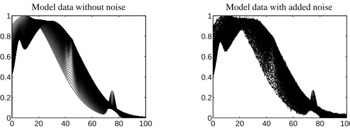
Figure 1: Model data with and without noise of a three-component system in order to illustrate the polygonsFC,FS,ICandIS and their pendants for noisy data. Left: The model data set from [5] for k=1000, n=500. Right: The data after application of normal distributed pseudo random noise with mean zero and a standard deviation of 0.01.
−0.4 −0.2 0 0.2 0.4 0.6
−0.5
−0.4
−0.3
−0.2
−0.1 0
FS andIS model data,MS ,∅
0 10 20
−80
−60
−40
−20 0 20
FCandICmodel data,MC,∅
Figure 2: Left plot: PolygonsFS(dashed) andIS (red). Right plot:FC(dashed) andIC(red). The polygons are plotted for the model data shown in the left subplot of Fig. 1. In the polygons INNPOL the data representatives aiand biare plotted in gray color. The AFS-setsMS andMCare nonempty.
Analogously the generalization ofFCwith respect to (10) for j=1 reads FeC=
(
y∈Rs−1: min
i=1,...,k
U(i,:)Σ(1,yT)T kUΣ(1,yT)Tk∞
≥ −εC )
. (14)
3.3. Computation ofFeS andFeC
The two polygonsFeS andFeCcan easily and precisely be computed by means of the polygon inflation algorithm (PIA). The idea of PIA is to approximate the boundary of a bounded set by a sequence of adaptively refined polygons.
The vertices of the polygons are located on the surface of the set. The boundary of the set is assumed to be locally representable by continuous functions. In [11] the PIA algorithm has been designed for AFS computations. Here PIA is used for the approximation of the polygonsFeS andFeC. This makes the computation very easy. In contrast to [11]
no complicated and computationally expensive target function must be evaluated. Instead, according to (6) and (9) a point x (resp. y) belongs to the surface of the FIRPOL polygons if V(1,x)T ≥0 (resp. UΣ(1,y)T ≥0) and V(1, ηx)T (resp. UΣ(1, ηy)) contains at least one negative component forη >1. More generally, for the noisy-data case the zero transition for changingηturns into a−εS or−εCtransition. Again, an adaptive polygon refinement strategy enables a highly accurate boundary approximation. All this makes the computational costs low.
5
−0.4 −0.2 0 0.2 0.4 0.6
−0.5
−0.4
−0.3
−0.2
−0.1 0
FS andIS for noisy data,MS =∅
0 10 20
−80
−60
−40
−20 0 20
FCandICfor noisy data,MC=∅
−0.4 −0.2 0 0.2 0.4 0.6
−0.5
−0.4
−0.3
−0.2
−0.1 0
FeS andeIS for noisy data,MfS ,∅
0 10 20
−80
−60
−40
−20 0 20
e
FCandIeCfor noisy data,MfC,∅
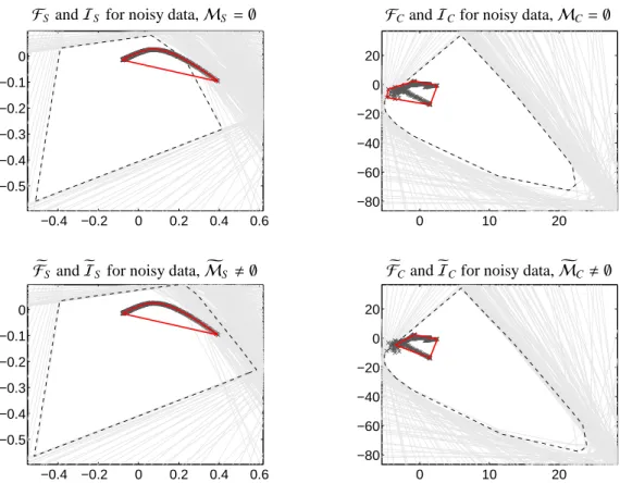
Figure 3: The polygons FIRPOL and INNPOL are drawn for the data set with noise as shown in the right subplot of Fig. 1. The two upper subplots demonstrate that INNPOLI(red) is not a subset of FIRPOLF(dashed) for these data. Hence the AFS is empty, i.e. no nonnegative factorization of D exists. The two lower plots show the generalized polygonsFeandeIeach for the factors C and S . The AFS-setsMS andMCare nonempty.
The boundary lines to strict nonnegativity with x1Vj2+x2Vj3=−V j1, j=1, . . . ,n, resp. y1σ2Ui2+y2σ2Ui3=−σ1Ui1, i=1, . . . ,k, are plotted in faint gray color. The data representing points ai, i=1, . . . ,k resp. bj, j=1, . . . ,n are plotted in the INNPOL polygons as by gray crosses.
3.4. Generalization of INNPOL for noisy data
The duality theory in [5, 12, 19, 20] describes how a point on the boundary of the polygonFCrelates to an affine hyperplane which touches the dual inner polygonIS. Further, Theorem 3.6 of [5] proves that a vertex ofFCrelates to a (true) facet ofIS. Our aim is to use these duality relations in order to construct from the boundary of the generalized set FIRPOLFeC the dual seteIS. HenceIeS is constructed by exploiting the duality relations. A direct construction by taking the convex hull of the vectors ai, i=1, . . . ,k, only results inIS and is not consistent with the weakened nonnegativity constraint.
The construction ofeIS is based on its duality to FeC. The duality relation of a point z to its dual hyperplane E = {y ∈ Rs−1 : yTz = −1}is introduced in Def. 3.1 in [5]. In Lemma 3.3 and Theorem 3.5 of [5] the focus is on duality of boundary points ofFeC to tangential hyperplanes ofeIS in order to constructFeC from eIS. However, the duality of polygons is an involutory mapping which relates in the same way the boundary ofeIS to tangential hyperplanes ofFeC. Thus the polygonIeS can be defined as
eIS =n
x∈Rs−1: the dual hyperplane E of x has an empty intersection with the interior ofFeC
o. (15)
Equivalently, the empty intersection of E with the interior ofFeCcan be expressed in a way that E has either an empty intersection withFeCor at most touches its boundary. An alternative way to write this polygon is
e
IS =closure({x∈Rs−1: E∩FeC =∅for E being the dual affine hyperplane of x}), 6
where closure denotes the topological closure of a set, i.e. the set augmented by all its limit points. Analogously, the set
e IC=n
y∈Rs−1: the dual hyperplane E of y has an empty intersection with the interior ofFeSo
(16) is the pendant of the polygonICfor the case of noisy data.
3.5. Computation ofeIS fromFeC
Numerically, we computeIeS by constructing the dual points of the edges of the convex hull ofFeC. These relations are illustrated in Figs. 1 and 2 in [5]. Alternatively, one can compute for the vertices of the convex hull ofFeC the associated dual half-spaces which are oriented in a way that each includes the origin; see Lemma 3.5 in [5]. The intersection of all these half-spaces yieldseIS (and is close to the initial polygonIS).
The figures 1, 2 and 3 illustrate the polygonsIS andIC and their noisy data pendants for the three-component model problem described in [5]. The dimensions are k = 1000 and n = 500. First Fig. 1 shows (a subset of) the series of spectra without and with noise. We have added normal distributed pseudo random noise with mean zero and a standard deviation of 0.01. It holds for the relative componentwise minimum/maximum that min(D)/max(D) =
−3.3·10−2and for the rank-3 approximation that
kD−UΣ(:,1 : 3)V(:,1 : 3)TkF kDkF
=1.6644·10−2. (17)
For the noise-free case Figure 2 illustrates the polygonsFSandIS as well asFCandICtogether with their generating boundary lines (aroundFC) and generating points (the gray stars inIS). Finally, Fig. 3 shows the situation for noisy data. First the polygons are drawn without any consideration for the perturbed data. Then no triangle exists in FIRPOL which includes INNPOL. Consequently the AFS-setsMS andMCare empty. Further the generalized noise-adapted polygonsFeS andeIS resp.FeCandIeCare plotted. For these polygons the AFS-setsMfS andMfCare nonempty. We have to show that these sets are good approximations ofMSandMCfor the case of noisy/perturbed data, see Sec. 4.5.
Remark 3.1. 1. The computational costs for a numerical approximation ofFeS andFeC by the polygon inflation algorithm are small, see Sec. 3.3.
2. For the computation ofFeC a precise boundary approximation is recommended in order to guarantee a stable subsequent application of the duality principles for the computation ofeIS. The control parameterεb on the boundary precision is explained in Sec. 3.9.1 of [10]. A reasonable parameter choice isεb≤10−6.
3. The control parameterεClimits the relative magnitude of negative entries of C according to (10); the parameter εS works similarly for the factor S . Increasing the value ofεS results in an expansion of FeS and thus in a shrinkage of the dual polygoneIC. (The shrinkage ofeIC is a consequence of Lemma 3.3 in [5] as the inner points ofIeC are dual to hyperplanes which do not contribute to the boundary of FeS and vice versa.) The geometric construction process shows thatMfS is expanded at the outer boundary and thatMfCis expanded at its inner boundary. Similarly, increasing the value ofεCresults in an expansion ofFeCand in a shrinkage of the dual polygoneIS. Thus the setMfS grows at its inner boundary andMfCgrows at the outer boundary. These relations are illustrated for example by Figure 6 in [3], Figure 17 in [9] and Figure 15 in [8].
For noisy data εC andεS should not be chosen too small as otherwise no feasible factorizations exist that meet the conditions. Then the AFS is empty. It is an interesting question which parameter selections can yield isolated feasible solutions; see [26] for the so-called data-based uniqueness in the noisy data case.
We cannot recommend a fixed rule how to determine the values ofεS andεC. The FACPACK software always tries to use small parameter values. The polygon inflation algorithm first tries to compute a strict-nonnegative matrix factorization (NMF) of D in a way that the smallest entries of its factors are equal to or greater than 0.
However, if no initial strict NMF can be found in this optimization process, then small positive values ofεS and εCmust be accepted. In other words, small matrix elements close to zero are accepted. If in such a case these parameters are equal to the smallest possible values so that an NMF exists, then at least one subset of the AFS is often very small. Then it cannot be guaranteed that the AFS includes the chemically correct solution. In this work we useεS =εC =5·10−2for the model problem from [5] which corresponds to the value of the rank-3 approximation error (17).
7
2000 2050 2100 0 0 500
0.02 0.04 0.06
wavenumber [cm−1]time [min]
absorption
0 200 400 600 800
0
time [min]
non-scaledconcentration
2000 2050 2100
0
wavenumber [cm−1]
non-scaledspectra
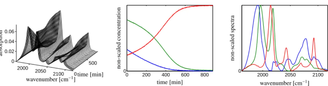
Figure 4: The experimental hydroformylation data set together with the pure component factors. Left: Every 25th spectrum of the 850 spectra is plotted. Center: The true concentration profiles computed by kinetic modeling. Right: The true pure component spectra. Color coding: Olefin (blue), acyl complex (green), hydrido complex (red).
3.6. Geometric AFS construction
Finally, the boundary curves of the AFS-sets MS andMC are determined. This is done by the simultaneous geometric construction algorithm, see the first part of this paper [5]. The only difference is that the algorithm is applied toFeS,FeCandeIS instead ofFS,FCandIS. The algorithm yields the inner parts of the boundary curves of the two AFS-sets. The outer parts of the boundary curves are given by parts of the boundaries ofFeS andFeC. The construction of the polygonsMfCandMfS is based on the inequalities (10). The same constraints are used in order to compute the FIRPOL polygons by the polygon inflation algorithm. Thus the inner and outer parts of the boundary are fitting to one another for the case of noisy data.
3.7. Non-convexity ofFeS
The acceptance of small negative entries of C and S may have the consequence that the polygonsFeS andFeC lose their convexity. Non-convexity is an unwanted side effect. On the one hand the non-convexity ofFeCresults in problems in the duality-based construction ofeIS. On the other hand the triangle rotation process for the simultaneous AFS construction, which determines the points of intersection of tangents ofeIS with boundary of the surrounding polygon FeS, can find more than two points of intersection in the case of a non-convex set FeS. Then additional steps are required in the program implementation in order to select the correct points of intersection. In our program implementation we avoid such problems with “slightly” non-convex sets in a way that we always work with the convex hulls ofFeresp.FeC.
4. Numerical results
The new algorithm is tested for an FT-IR experimental data set from the hydroformylation process. For this noise- including data set we first draw the polygonsFe,FeC andeIS. The series of spectra has undergone a background subtraction and a baseline correction. After this, the simultaneous geometric construction yields the AFS-setsMS andMC. These AFS-sets are compared to the corresponding approximations by the FACPACK software. Further the results are compared to the generalized Borgen plots. The results are analyzed and the computation times are discussed. All computations were run on a PC with an Intel 3.40GHz quad-core processor and 16GB RAM. The main algorithm is implemented in fast C-routines. The program is executed on a single core of the processor.
4.1. Rhodium catalyzed hydroformylation
From the series of 850 FT-IR spectra only a spectral window with 645 spectral channels is considered. Thus D∈ R850×645. The associated time and wavenumber intervals are t∈[4.7,883.6]min andν∈[1962.3, 2117.6]cm−1. Three major absorbing components contribute to the spectra, namely an olefin component, an acyl complex and a hydrido complex. The reaction product, an aldehyde, shows no absorption in the spectral window. For the experimental details see [27]. The series of spectra and the true pure component spectra and concentration profiles, which are computed by using additionally a kinetic model, are presented in Fig. 4.
8
−3 −2 −1 0 1 2
−30
−20
−10 0 10 20
y1
y2
PolygonsFCvs.FeCandICvs.IeC
−0.5 0 0.5 1
−0.2 0 0.2 0.4 0.6 0.8 1 1.2
x1 x2
PolygonsFS vs.FeS andIS vs.IeS
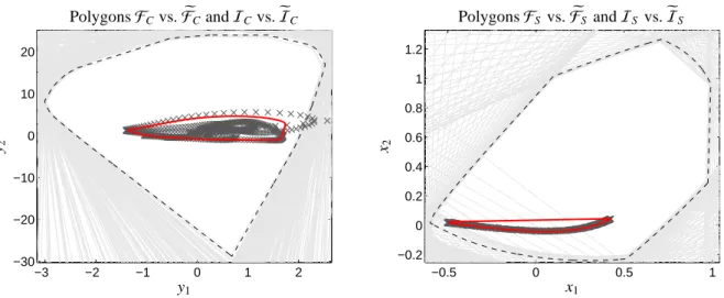
Figure 5: Comparison of the polygonsF andIand their pendants for partially negative dataFeandeIeach for C and S . Left: The polygonsFeC (black broken line) andeIC(red line). The gray lines define the boundary ofFCand the dark gray crosses are the data representing vectors bj, j=1, . . . ,n. Right: The polygonsFeS (black broken line) andeIS (red line) are drawn. The gray lines define the boundary ofFS and intersect in the left lower region the polygonFeS. The dark gray crosses represent the data vectors ai, i=1, . . . ,k. The left plot illustrates major differences betweeneICandIC. The triangle rotation algorithm applied toFCandICwould result in an empty AFSMC. A similar situation is illustrated in the right plot, whereISintersectsFS. In particular two half-spaces (by the gray lines) in the right plot do not include the origin due to the fact that min(D)=−4.8·10−4.
Due to a background subtraction and also due to a subsequent SVD-based low-rank approximation the matrix D includes small negative entries. The smallest matrix entry of D is min(D)=−4.8·10−4. The relative size of the smallest matrix entry equals min(D)/max(D)=−6.5·10−3; the minimum and the maximum are taken componentwise.
Further, the relative error of the rank-3 approximation of D reads kD−CSTkF
kDkF
= sPn
i=4σ2i Pn
i=1σ2i =5.995·10−3 (18)
with C and S containing columnwise expansions with respect to the first s = 3 left- and right singular vectors.
The “true” pure components are computed by adding a kinetic Michaelis-Menten hard model, cf. [28, 29, 30]. The ssq-deviations of the Michaelis-Menten solutions C(ode)from the pure component factor are computed as
di=kC(ode)(:,i)−α(UΣ(1,y1(i),y2(i))Tk22 kC(ode)(:,i)k22
with norm-minimizing scaling constantsα. The numerical values are (2.2·10−4,5.2·10−5,1.5·10−4) for the three components.
4.2. FIRPOL, INNPOL and parameter setting
First the polygonsFeS andFeC are computed by polygon inflation with the control parametersε = εS = εC = 6.0·10−3as lower bounds for the relative sizes of negative entries in C and S , see Eqns. (13) and (14). See [10, 11]
for the details on these control parameters. Then the duality theory in [5] is the basis to compute fromFeC the inner polygoneIS for the case of noisy data, see Sec. 3.5.
Figure 5 shows the FIRPOL and INNPOL polygons for the hydroformylation data set together with their pendants for slightly negative data. Additionally, the spectral data representing vectors ai, i=1, . . . ,k, and the bj, j=1, . . . ,n are plotted. The gray straight lines represent the affine half-spaces whose intersections define the FIRPOL polygons FS andFC. The left subplot in Figure 5 highlights that the data representatives and thus their convex hull INNPOL intersect FIRPOL. The consequence is an empty AFS. However, the smaller and modified seteIC(in red) is completely
9
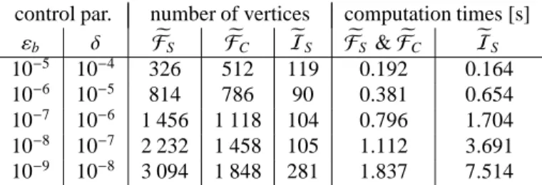
control par. number of vertices computation times [s]
εb δ FeS FeC IeS FeS &FeC eIS
10−5 10−4 326 512 119 0.192 0.164
10−6 10−5 814 786 90 0.381 0.654
10−7 10−6 1 456 1 118 104 0.796 1.704 10−8 10−7 2 232 1 458 105 1.112 3.691 10−9 10−8 3 094 1 848 281 1.837 7.514
Table 1: Computation times forFeSandFeCand for the duality based construction ofIeS fromFeCfor different precisionsεband different stopping criteriaδof polygon inflation. The parameterεbcontrols the accuracy of the boundary approximation. The stopping criteriaδcontrols the number of edges, see [10, 11, 31]. We useδ=10εb.
number of tangents contr. param. number of vertices computation times [s] forMfS andMfC
minit mall εb δ MfS MfC FeS,FeC,IeS geom. constr. Total comp. time
1 500 3 206 10−6 10−5 3 445 6 091 1.035 0.143 1.172
2 500 5 495 10−7 10−6 5 982 10 267 2.500 0.378 2.878
5 000 7 995 10−7 10−6 7 964 14 229 2.500 0.570 3.070
10 000 14 530 10−8 10−7 14 007 25 184 4.803 1.348 6.151
15 000 19 530 10−8 10−7 17 968 33 105 4.803 2.003 6.806
Table 2: The computation times of the dual Borgen plot method are listed for different numbers of tangents and different precision parametersεb. The computation times for computing the polygonsFeS,FeCandeISas well as the times for the construction of the two dual AFS-sets are tabulated separately. The parameter setting minit=2500 andεb=10−7is sufficient for a high-resolution computation.
contained inFeC. The right subplot of Figure 5 shows two gray straight lines which bound two half-spaces which do not include the origin. By the mathematical theory this is only possible if DTD is an reducible matrix or if D includes negative entries. Here it holds componentwise that min(D)=−4.8·10−4. In particular the first right singular vector contains positive and also two small negative entries (whereas for D≥0 the Perron-Frobenius theory guarantees that the first singular vector can be selected nonnegative. By the modified definition ofFeS this unwanted effect disappears.
With the parametersεb=10−7andδ=10−6, see the FACPACK manual, the polygonFeS has 1456 vertices andFeC
has 1118 vertices. The duality theory allows us to constructeIS from givenFeC. ThenIeS has only 104 vertices. The much smaller number of vertices ofeIS is due to the fact that the convex hull ofFeCis used for the dual construction, see Sec. 3.7. This has characteristically reduced the number of vertices. Finally, the inner polygoneIC has 236 vertices. Figure 5 shows the polygons for a fixed set of control parameters. Table 1 lists the computation times for other parameter selections. The computation is still very fast forεb andδclose to zero, which results in a larger number of vertices of the polygons.
4.3. Geometric construction of the dual AFS-sets
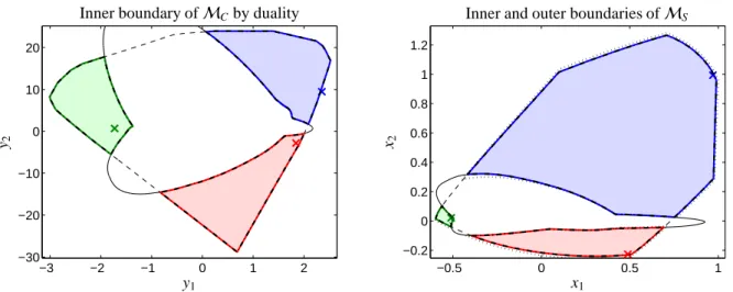
The final step is the simultaneous geometric construction of the inner boundaries of the AFS-setsMS andMC. The construction algorithm is explained in the first part of this paper [5]. The only difference is that FS,FC and IS are substituted byFeS, FeC andeIS. We use the control parametersεb = 10−7 andδ = 10−6. The resulting AFS-sets are shown in Fig. 6. These AFS-sets are plotted together with the approximations by the polygon inflation based AFS computation by FACPACK and also with the results by the generalized Borgen plots algorithm. The first two approximations coincide, but there are small differences to the generalized Borgen plots, see Fig. 6. The “true solution” (by kinetic hard-modeling) are marked by bold colored crosses. The dual Borgen plot uses a rotation angle increment of 360◦/5000=0.072◦and some additional tangents, especially those which cover edges ofIeS. The total number of used tangents is 7995. The geometric construction by duality takes 0.570s and the overall dual Borgen plot construction takes 3.070s.
10
−3 −2 −1 0 1 2
−30
−20
−10 0 10 20
y1
y2
Inner boundary ofMCby duality
−0.5 0 0.5 1
−0.2 0 0.2 0.4 0.6 0.8 1 1.2
x1
x2
Inner and outer boundaries ofMS
Figure 6: The AFS-setsMCandMS for the experimental spectral data set. The three isolated subsets for each of the two AFS-sets by the dual Borgen plot method are drawn in green, red and blue. The colored x-markers represent the Michaelis-Menten hard modeling results as plotted in Fig. 4. The residuals for all solutions in the AFS has the fixed value 5.995·10−3by Eq. (18). Their boundaries coincide with the dash-dotted lines which are the boundaries of the AFS approximations by the polygon inflation based AFS computation with the FACPACK software. Dotted black lines: The right figure also shows the AFS approximation by the generalized Borgen plot algorithm. Minor differences can be seen at the boundary of the blue set. Additionally the setsFeandFeCare marked by broken black lines. The inner boundaries of the AFS-sets are plotted in black.
contr. param. number of vertices computation times [s] FACPACK-PIA
εb δ MfS MfC MfS MfC MfS andMfC
10−3 10−3 261 295 8.725 13.019 21.744
10−4 10−3 271 299 12.389 17.033 29.422
10−4 10−4 679 663 27.055 30.605 57.660
10−5 10−4 669 663 37.768 39.743 77.511
Table 3: The computation times are tabulated of the FACPACK-based AFS computation by the polygon inflation algorithm (FACPACK-PIA). The times are considerably larger than those of the dual Borgen plot construction, see Table 2. The boundaries of the AFS-sets by the two methods coincide apart from small deviations of the size of the control parameterεb.
4.4. Variation of the number of tangents
The dual Borgen plot construction is run with different numbers of tangents. For the computations we use initial numbers minitof 1500, 2500, 5000, 10000 and 15000 tangents; consecutive tangents enclose a fixed rotation angle.
These tangents are augmented to a total number mallof tangents. These additional tangents primarily refer to edges of eIS by the duality relations. The computation times for the polygon constructions and for the following duality-based simultaneous AFS construction are listed in Table 2. The computation times remain to be in the range of few seconds even for the highest resolution. These results are to be compared with alternative methods for AFS computations.
4.5. Comparison of the results
The AFS-setsMfS andMfCfor perturbed/noisy data are compared to FACPACK based AFS computation by the polygon inflation algorithm (FACPACK-PIA) and also to the generalized Borgen plots (GBP). For these comparisons we consider different choices of the control parameters.
4.5.1. Comparison to polygon inflation method
Table 3 contains the computing times for the AFS computations by FACPACK-PIA for different settings of the boundary precisionεb and the stopping criteriaδ. Even for the default control parameter settingsεb = δ = 10−3 FACPACK-PIA requires about 21.7s for the computation ofMfS andMfC. In contrast to this, the dual Borgen plot method even with a smaller control parameter and with a number of 5000 initial tangents takes only about 3s. Hence
11
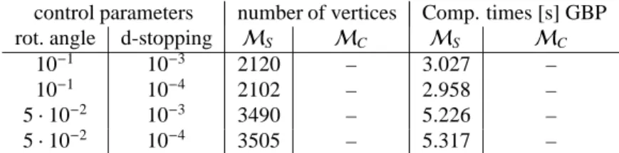
control parameters number of vertices Comp. times [s] GBP
rot. angle d-stopping MS MC MS MC
10−1 10−3 2120 – 3.027 –
10−1 10−4 2102 – 2.958 –
5·10−2 10−3 3490 – 5.226 –
5·10−2 10−4 3505 – 5.317 –
Table 4: Computation times of the generalized Borgen plot (GBP) method. The numbers of computed tangents are comparable to the dual Borgen plot method, see Table 2, but much smaller than those of FACPACK-PIA, see Table 3. The AFSMCcannot be computed with GBP as the magnitude of negative components is too large.
the dual Borgen plot construction is about 7 times faster than the (already fast) FACPACK-PIA method. The precision of the results is not affected. The AFS approximations by these methods coincide aside from differences of the magnitude of the boundary precisionεb.
The high efficiency of the dual Borgen plot method can be explained by the fact that it immediately accesses the structure-forming objects, namely the polygons FIRPOL and INNPOL. In contrast to this, the optimization based FACPACK-PIA algorithm explores for each subset of the AFS its boundary by using an adaptive approximation algo- rithm. This also explains why FACPACK-PIA detects a characteristically smaller number of vertices, see Tables 2, 3 and 4. However, the smaller number of vertices does not affect the precision of the boundary approximation which is controlled by the parameterεbas the non-detected vertices belong to pairs of edges which are nearly collinear.
4.5.2. Comparison to generalized Borgen plots
Table 4 contains the computation times and number of vertices for the approximate construction ofMS by the generalized Borgen plot (GBP) method. For the default control parameter settingsrot. angle=0.1 andd-stopping=
10−3the computation ofMS is completed within 3s. The resulting AFS-sets by GBP are slightly different to the AFS-sets by the dual Borgen plot method due to the different approach to use absolute lower bounds on the acceptable negative matrix entries compared to the relative bounds (10). Further GBP cannot compute the AFSMCsince the magnitude of negative entries in this experimental data set is too large.
5. Conclusion
MCR methods should be suitable for applications to experimental spectral data including noise, perturbations, baseline drifts and other types of errors and nonlinearities. Data preprocessing steps as baseline corrections, back- ground subtractions or noise-reducing low-rank approximations can introduce small negative entries to the spectral data set. The classical Borgen plots by Borgen and Kowalski cannot handle such data with small negative entries.
The present paper devises a way on how to work with small negative data entries in the dual Borgen plot con- structions. The idea is to map the weakened nonnegativity constraints to two modified, namely increased, polygons FIRPOL, which represent in the classical Borgen plot construction exactly the nonnegativity constraints. For given FIRPOL, duality principles help to construct a corresponding modified polygon INNPOL. This reorganized construc- tion of the polygons INNPOL and FIRPOL, which are nesting sets of the AFS, is followed by the dual Borgen plot construction as introduced in the first part of this paper [5]. The resulting overall process combines the elegance of the geometric Borgen plot construction with the numerical robustness of the optimization-based AFS computation methods as triangle enclosure [7], polygon inflation [10, 11] and ray casting [15].
The approach to map the weakened nonnegativity constraint to a modified definition of the polygon FIRPOL makes it possible to implement not only lower bounds on the relative size of negative matrix entries (as used here), but also to use absolute lower bounds as done in the generalized Borgen plot (GBP) method. In general, constraint implementation via a re-definition of the polygons FIRPOL and INNPOL in the Borgen plot constructions appears to be a challenging research topic.
12
References
[1] O.S. Borgen and B.R. Kowalski. An extension of the multivariate component-resolution method to three components. Anal. Chim. Acta, 174:1–26, 1985.
[2] R. Rajk´o and K. Istv´an. Analytical solution for determining feasible regions of self-modeling curve resolution (SMCR) method based on computational geometry. J. Chemom., 19(8):448–463, 2005.
[3] A. J ¨urß, M. Sawall, and K. Neymeyr. On generalized Borgen plots. I: From convex to affine combinations and applications to spectral data.
J. Chemom., 29(7):420–433, 2015.
[4] A. Meister. Estimation of component spectra by the principal components method. Anal. Chim. Acta, 161:149–161, 1984.
[5] M. Sawall, A. J ¨urß, H. Schr¨oder, and K. Neymeyr. Simultaneous construction of dual Borgen plots. I: The case of noise-free data. Technical report, To appear in J. Chemom., DOI: 10.1002/cem.2954., 2017.
[6] A. Golshan, H. Abdollahi, S. Beyramysoltan, M. Maeder, K. Neymeyr, R. Rajk´o, M. Sawall, and R. Tauler. A review of recent methods for the determination of ranges of feasible solutions resulting from soft modelling analyses of multivariate data. Anal. Chim. Acta, 911:1–13, 2016.
[7] A. Golshan, H. Abdollahi, and M. Maeder. Resolution of rotational ambiguity for three-component systems. Anal. Chem., 83(3):836–841, 2011.
[8] A. J ¨urß, M. Sawall, and K. Neymeyr. On generalized Borgen plots. II: The line-moving algorithm and its numerical implementation. J.
Chemom., 30:636–650, 2016.
[9] M. Sawall, A. J ¨urß, H. Schr¨oder, and K. Neymeyr. On the analysis and computation of the area of feasible solutions for two-, three- and four- component systems, volume 30 of Data Handling in Science and Technology, “Resolving Spectral Mixtures”, Ed. C. Ruckebusch, chapter 5, pages 135–184. Elsevier, Cambridge, 2016.
[10] M. Sawall, C. Kubis, D. Selent, A. B¨orner, and K. Neymeyr. A fast polygon inflation algorithm to compute the area of feasible solutions for three-component systems. I: Concepts and applications. J. Chemom., 27:106–116, 2013.
[11] M. Sawall and K. Neymeyr. A fast polygon inflation algorithm to compute the area of feasible solutions for three-component systems. II:
Theoretical foundation, inverse polygon inflation, and FAC-PACK implementation. J. Chemom., 28:633–644, 2014.
[12] S. Beyramysoltan, H. Abdollahi, and R. Rajk´o. Newer developments on self-modeling curve resolution implementing equality and unimodal- ity constraints. Anal. Chim. Acta, 827(0):1–14, 2014.
[13] M. Vosough, C. Mason, R. Tauler, M. Jalali-Heravi, and M. Maeder. On rotational ambiguity in model-free analyses of multivariate data. J.
Chemom., 20(6-7):302–310, 2006.
[14] H. Abdollahi and R. Tauler. Uniqueness and rotation ambiguities in Multivariate Curve Resolution methods. Chemom. Intell. Lab. Syst., 108(2):100–111, 2011.
[15] M. Sawall and K. Neymeyr. A ray casting method for the computation of the area of feasible solutions for multicomponent systems: Theory, applications and FACPACK-implementation. Anal. Chim. Acta, 960:40–52, 2017.
[16] W.H. Lawton and E.A. Sylvestre. Self modelling curve resolution. Technometrics, 13:617–633, 1971.
[17] H. Schr¨oder, M. Sawall, C. Kubis, D. J ¨urß, A. Selent, A. Br¨acher, A. B¨orner, R. Franke, and K. Neymeyr. Comparative multivariate curve resolution study in the area of feasible solutions. Chemom. Intell. Lab. Syst., 163:55–63, 2017.
[18] H. Minc. Nonnegative matrices. John Wiley & Sons, New York, 1988.
[19] R.C. Henry. Duality in multivariate receptor models. Chemom. Intell. Lab. Syst., 77(1-2):59–63, 2005.
[20] R. Rajk´o. Natural duality in minimal constrained self modeling curve resolution. J. Chemom., 20(3-4):164–169, 2006.
[21] M. Sawall and K. Neymeyr. On the area of feasible solutions and its reduction by the complementarity theorem. Anal. Chim. Acta, 828:17–26, 2014.
[22] M. Sawall, C. Kubis, R. Franke, D. Hess, D. Selent, A. B¨orner, and K. Neymeyr. How to apply the complementarity and coupling theorems in MCR methods: Practical implementation and application to the Rhodium-catalyzed hydroformylation. ACS Catal., 4:2836–2843, 2014.
[23] K. Neymeyr and M. Sawall. On an SVD-free approach to the complementarity and coupling theory: A note on the elimination of unknowns in sums of dyadic products. J. Chemom., 30:30–36, 2016.
[24] H. Abdollahi, M. Maeder, and R. Tauler. Calculation and Meaning of Feasible Band Boundaries in Multivariate Curve Resolution of a Two-Component System. Anal. Chem., 81(6):2115–2122, 2009.
[25] A. Golshan, M. Maeder, and H. Abdollahi. Determination and visualization of rotational ambiguity in four-component systems. Anal. Chim.
Acta, 796(0):20–26, 2013.
[26] R. Rajk´o, H. Abdollahi, S. Beyramysoltan, and N. Omidikia. Definition and detection of data-based uniqueness in evaluating bilinear (two- way) chemical measurements. Anal. Chim. Acta, 855:21 – 33, 2015.
[27] C. Kubis, M. Sawall, A. Block, K. Neymeyr, R. Ludwig, A. B¨orner, and D. Selent. An operando FTIR spectroscopic and kinetic study of carbon monoxide pressure influence on rhodium-catalyzed olefin hydroformylation. Chem.-Eur. J., 20(37):11921–11931, 2014.
[28] M. Maeder and Y.M. Neuhold. Practical data analysis in chemistry. Elsevier, Amsterdam, 2007.
[29] M. Sawall, A. B¨orner, C. Kubis, D. Selent, R. Ludwig, and K. Neymeyr. Model-free multivariate curve resolution combined with model-based kinetics: Algorithm and applications. J. Chemom., 26:538–548, 2012.
[30] H. Schr¨oder, M. Sawall, C. Kubis, D. Selent, D. Hess, R. Franke, A. B¨orner, and K. Neymeyr. On the ambiguity of the reaction rate constants in multivariate curve resolution for reversible first-order reaction systems. Anal. Chim. Acta, 927:21–34, 2016.
[31] M. Sawall, A. J ¨urß, and K. Neymeyr. FACPACK: A software for the computation of multi-component factorizations and the area of feasible solutions, Revision 1.3. FACPACK homepage: http://www.math.uni-rostock.de/facpack/, 2015.
13