Simultaneous construction of dual Borgen plots. I: The case of noise-free data

Simultaneous construction of dual Borgen plots.

I: The case of noise-free data

Mathias Sawall^a, Annekathrin J¨urß^a, Henning Schr¨oder^a,b, Klaus Neymeyr^a,b

aUniversit¨at Rostock, Institut f¨ur Mathematik, Ulmenstrasse 69, 18057 Rostock, Germany

bLeibniz-Institut f¨ur Katalyse, Albert-Einstein-Strasse 29a, 18059 Rostock

Abstract

In 1985 Borgen and Kowalski [DOI:10.1016/S0003-2670(00)84361-5] introduced a geometric construction algorithm for the regions of feasible nonnegative factorizations of spectral data matrices for three-component systems. The resulting Borgen plots represent the so-called Area of Feasible Solutions (AFS). The AFS can be computed either for the spectral factor or for the factor of the concentration profiles. In the latter case, the construction algorithm is applied to the transposed spectral data matrix. The AFS is a low-dimensional representation of all possible nonnegative solutions, either of the possible spectra or of the possible concentration profiles.

This work presents an improved algorithm for the simultaneous construction of the two dual Borgen plots for the spectra and for the concentration profiles. The new algorithm makes it possible to compute the two Borgen plots roughly at the costs of a single classical Borgen plot. The new algorithm comes without any loss of precision or spatial resolution. The new method is benchmarked against various program codes for the geometric-constructive and for the numerical optimization-based AFS computation.

Key words: multivariate curve resolution, Borgen plot, nonnegative matrix factorization, area of feasible solutions, polygon inflation, FACPACK.

1. Introduction

In model-free multivariate curve resolution (MCR) the aim is to extrapolate from the spectral observation of a chemical reaction system to the contributions from the underlying pure components. If a series of spectra is measured and if these spectra are written as the rows of a k-by-n spectra matrix D, then the Lambert-Beer law

D=CS^T+E (1)

expresses an approximate bilinear relation between D and the nonnegative factors C ∈ R^k×s and S ∈ R^n×s. The error term E is assumed to be small or to vanish.

The columns of C are the concentration profiles of the s pure components and the columns of S are the associ- ated pure component spectra [15, 14]. If only D is given, then the computation of chemically interpretable factors C and S is a difficult problem as (1) with E=0 can have many nonnegative solutions. This fact is known under the keyword rotational ambiguity, see e.g. [34, 2]. Ad- ditional information on the reaction system can help to reduce this ambiguity. Here we pursue the approach to

compute the complete range of all nonnegative factor- izations D =CS^T and to represent the possible factors columnwise in the low-dimensional form of the Area of Feasible Solutions (AFS). Such AFS analyses are well- known for two-, three- and four-component systems.

These techniques can be classified as either geometric constructive approaches [13, 16, 5, 23, 11] or as nu- merical optimization-based approaches [1, 7, 27, 8, 31].

In recent years many new methods or modifications of established methods have been devised; see the review works [6, 26]. Some of these methods have reduced the computational costs for determining the AFS con- siderably. The computation times are about seconds for medium-sized data sets and are up to minutes for multi- megabyte data sets.

1.1. Motivation and aim of the paper

Against the background of an increasing importance of model-free MCR methods, which are always faced with the problem of the non-uniqueness of their results due to the so-called rotational ambiguity, we present a new, very efficient algorithm which simultaneously con- structs the AFS sets for the concentration factor and

for the spectral factor. This new algorithm is based on a geometric construction in terms of Borgen plots [16, 5, 23, 22, 11, 12]. It does not include any numer- ical approximations. Therefore the algorithm provides precise results - however, small rounding errors are un- avoidable if the algorithm is implemented on a com- puter. As is typical for Borgen plots, the algorithm can only be applied to non-perturbed and noise-free model data. This disadvantage will be compensated in a forth- coming second part of this paper, where the algorithm is extended in a way that it can be applied to perturbed, noisy experimental spectral data. This extended algo- rithm is of a hybrid nature, as it combines the geometric construction with the numerical approximation under- lying the polygon inflation algorithm [27, 28]. The new methods work accurately and are very fast.

In this first part, we analyze a certain duality of the polygons INNPOL and FIRPOL, see Sec. 3 and [10, 21]. This duality can be used in a way that a facet of INNPOL for the one factor makes it possible to con- struct a vertex of FIRPOL for the other factor. Such a duality is already known in the community. What is new is that the duality is exploited in order to build a fast and precise construction of the AFS for the concen- tration factor and simultaneously for the spectral factor.

For each constructed boundary point of the AFS of one factor the new method forms two inner boundary points of the AFS for the other factor. Our analysis is partially general in a sense that it applies to any dimension. Then INNPOL and FIRPOL are polyhedra. The forthcom- ing second part of the paper combines the speed and precision of the geometric construction with the robust- ness for perturbed and noisy data of optimization-based methods. Such a robustness is the benefit of the nu- merical AFS computation methods as polygon inflation, triangle enclosure or grid-search. The new algorithm si- multaneously computes the two AFS sets almost as fast as the classical Borgen plot algorithm computes a single AFS for ideal model data.

1.2. Organization of the paper

The paper is organized as follows: Sec. 2 introduces the SVD-based approach to to MCR problem and to the AFS. Sec. 3 defines certain important sets and polyhe- dra for the subsequent geometric constructions, contains their analysis and presents an indirect and very fast com- putation method, which is based on the complementar- ity/duality theory. The central new results on the si- multaneous geometric construction of the AFS sets for noise-free data are presented in Sec. 4. Finally, the re- sults are compared to the results of other methods (poly- gon inflation and generalized Borgen plots) in Sec. 5.

1.3. Notation

The following notation is used in the paper.

D k×n spectral data matrix by Eqs. (1), (2).

C k×s concentration matrix by Eq. (1).

S n×s spectra matrix by Eq. (1).

UΣV^T singular value decomposition of D by Eq. (2).

T s×s transformation matrix by Eqs. (2), (3).

M AFS spectral factor by Eq. (4).

M_C AFS concentration factor by Eq. (5).

I INNPOL spectral factor by Eq. (8).

I_C INNPOL concentration factor by Eq. (9).

F FIRPOL spectral factor by Eq. (8).

F_C FIRPOL concentration factor by Eq. (9).

ai scaled left singular vectors by Eq. (6).

bj scaled right singular vectors by Eq. (7).

2. MCR and the AFS

A well-established approach to the construction of nonnegative factors C ∈R^k×sand S ∈R^n×sfor a given rank-s matrix D ∈ R^k×n is to use a singular value de- composition (SVD) D = UΣV^T of D, see [9]. Here we consider a truncated SVD in a way that U and V have only s columns and thatΣis an s-by-s diagonal matrix with the s dominant singular values of D on its diagonal. Then the product UΣV^Tis the best rank-s ap- proximation of D in the least-squares sense [9, 33]. The truncated SVD is important in the case of perturbed data with E ,0 in (1) so that D≈UΣV^T. For ease of pre- sentation we consider E=0 in the sequel. The key idea for the construction of C and S is to insert a transforma- tion T ∈R^s×sand its inverse in the truncated SVD in a way that

D=UΣV^T =UΣT⁻¹

| {z }

=C≥0

T V^T

|{z}

=S^T≥0

. (2)

Only those T are considered for which C and S are non- negative matrices. A purely numerical approach is to determine the matrix elements of T by solving an opti- mization problem, see e.g. [35, 19].

2.1. Sets of feasible spectra and concentration profiles If (2) holds for a certain T and P is a permutation matrix, then this equation holds also for PT instead of T (then T⁻¹ is substituted by T⁻¹P^T). This operation rearranges the columns of C and S in the same way.

Consequently the set of all possible first columns of S is equal to the set of all possible columns of S (i.e. the 2

possible spectra). We denote this set byS and the cor- responding set of possible concentration profiles byC so that

C ={u∈R^k: (2) holds with C(:,1)=u}, S ={3∈Rⁿ: (2) holds with S (:,1)=3}.

If an algorithm is available which allows us to deter- mine the setS, thenC can be formed by applying this algorithm to D^T =S C^T as C and S have changed their places by transposition. We call a spectrum3feasible if matrices C,S ≥0 exist so that3equals the first column of S and D=CS^T.

2.2. The AFS

The setS is unbounded as any positive multipleω3 for3 ∈S andω >0 is consistent with (2) if the asso- ciated u is substituted by u/ω. The unboundedness can easily be avoided by fixing a certain scaling. Therefore each matrix element in the first column of T is set equal to 1

T =



















1 x1 · · · xs−1

1

...

W

1



















. (3)

The justification that each vector in S has a non- vanishing contribution from the first right singular vec- tor relies on the Perron-Frobenius theory of nonnegative matrices [17], see [28] for the proof. This allows us to define the AFS as the set of the (s−1)-dimensional row vectors

M:={x∈R^s−1: exists W∈R(s−1)×(s−1)with

T (1,2 : s)=x^T,rank(T )=s and C,S ≥0} (4) with T and W by (3); see [7, 27, 26]. Some basic properties of the AFS, not only thatMis bounded and does not include the origin, are proved in [28, 11, 31].

These proofs require the (mild) assumptions that DD^T and D^TD are irreducible matrices.

The corresponding AFS for the factor C is defined as M_C ={y∈R^s−1: exists T ∈R^s×s,rank(T )=s,

(T⁻¹)(:,1)= 1 y

!

and UΣT⁻¹≥0,T V^T ≥0}. (5) 2.3. AFS computations

For two-component systems (s = 2) the AFS can explicitly be written in dependence on the matrix ele- ments of D, see [13, 2, 28, 26, 31]. For three- and four- component systems various and differing AFS compu- tation methods are available. As already mentioned in

Sec. 1, the algorithms for three-component systems are either of geometric-constructive nature [5, 23, 11] or are based on the solution of numerical optimization prob- lems [2, 7, 27, 31]. For four-component systems the pioneering work has been done in [8, 6, 26, 31].

The focus of this work is on three-component sys- tems. A new technique is developed which determines the (boundaries of the) setsMandM_Csimultaneously.

The details of this new method are explained in Sec. 4.

In the next, preparatory section we define and analyze two important supersets ofMandMC.

3. Fast computation of FIRPOL

This section deals with the polygons FIRPOL and INNPOL as introduced by Borgen and Kowalski [5]

and, e.g., later used in [23, 11]. Here the representa- tion is not restricted to polygons (s =3) but applies to polyhedra of arbitrary dimensions s≥3. The construc- tion of the polyhedra FIRPOL and INNPOL is the first step for the geometric construction of the spectral AFS Mand its pendantM_Cfor the concentration factor. In the following we describe and analyze various duality relations between the polyhedra FIRPOL and INNPOL for eachMandM_C. These results relate facets of IN- NPOL with vertices of FIRPOL. Finally, we describe an approach how the polyhedra FIRPOL (both for the spectral factor and for the concentration factor) can be computed in a fast indirect way.

The underlying duality relations are known, see Henry [10] and Rajk ´o [21]. The duality has been used in [3] for the effective construction of the polygons FIR- POL and INNPOL for the two factors. The decisive point of the duality analysis in this section is to show that extremal points of INNPOL are one-to-one related to halfplanes which include facets of the dual polygon FIRPOL. Similarly, inner points of INNPOL are also one-to-one related to dual halfplanes which do not con- tribute to the boundary of FIRPOL.

The duality is also expressed in some complementar- ity theory, see, e.g., [24, 30, 18]. However, a simultane- ous construction algorithm for Borgen plots, in which a single triangle rotation process is used in order to con- struct the two AFS sets by using duality relations, has not been described or published.

3.1. A remark on the duality principle

In general, duality in mathematics is a principle which refers to two (mathematical) objects which stand in a one-to-one relation. Properties of one of these ob- jects can often be translated to related properties of the 3

second object. Duality relations are well known in op- timization theory, mathematical logic, set theory and many other fields. In this paper, the term duality refers to various properties of the representing sets of two fac- tors C and S^T of D and their construction.

3.2. Data representation and affine hyperplanes In order to construct the boundaries ofMandM_C some auxiliary objects are required. The starting point is the SVD D = UΣV^T which can be written in the equivalent forms

DV=UΣ and Σ⁻¹U^TD=V^T.

The first equation can be interpreted in a way that it rep- resents the expansion coefficients of the ith row of D with respect to the basis of right singular vectors by the ith row of UΣ. The second equation is the correspond- ing or dual representation of the columns of D with re- spect to the basis of scaled (with the singular values) left singular vectors; the columns of V^Tcontain the ex- pansion coefficients. These vectors of expansion coeffi- cients together with the normalization as used in (3)–(5) are the (s−1)-dimensional column vectors

ai:=((UΣ)(i,2 : s))^T

(UΣ)(i,1) = (UΣ)^T(2 : s,i) U^T(1,i)σ1

(6) for i=1, . . . ,k and the column vectors

bj:=V^T(2 : s,j)

V^T(1,j) (7)

for j=1, . . . ,n.

Borgen and Kowalski [5] in their geometric construc- tion ofMfor the case s = 3 defined the polygonsF (called FIRPOL) andI(called INNPOL) by means of the aiand bj. For general s≥3, these polyhedra have the form

F ={x∈R^s−1: V 1 x

!

≥0}, I=convhull{a_i: i=1, . . . ,k},

(8)

see also [23, 11]. The definition of the analogous sets for the concentration factor C read

F_C={y∈R^s−1: UΣ 1 y

!

≥0}, IC =convhull{bj: j=1, . . . ,n}.

(9)

These latter sets are required for the construction of MC.

The superset FIRPOL, denoted by F, of M is by its definition the intersection of the n affine half-spaces which are given by the n components of the inequality V(1,x^T)^T ≥0. These n affine half-spaces are one-sided bounded by the n affine hyperplanes (which derive from the jth component of V(1,x^T)^T =0)

E^{(S )}_j :=

(

x∈R^s−1: V( j,2 : s)x V( j,1) =−1

)

(10) for j=1, . . . ,n. Analogously, the affine hyperplanes

E^(C)_i = (

y∈R^s−1: UΣ(i,2 : s)y U(i,1)σ₁ =−1

)

, (11)

for i = 1, . . . ,k belong to the affine half-spaces UΣ(1,y^T)^T ≥0. Each of these affine half-spaces is ori- ented in a way that it contains the origin. The intersec- tion of these spaces is the supersetF_CofM_C.

3.3. Duality of points and affine hyperplanes

Next relations fromI_CtoF are analyzed. Analogous relations hold for IandF_C. These relations and their analysis are the basis of the construction algorithms for F and F_C. The starting point for the analysis is the complementarity and coupling theory in [24]. This the- ory is closely related to the duality principles as stated by Henry [10] and Rajk ´o [21]. The duality describes mathematical constraints for the columns of C if certain columns of S are known and vice versa. The constraints are given in the form of (affine) linear equations for the unknown parts. Typically, the theory provides major re- strictions, i.e. small subsets of the AFS can be identi- fied which include the feasible solutions. For a discus- sion and for the analysis of the constraining conditions, see [21, 4, 30]. For example, a central result is that a fixed point in the AFSM(i.e. a certain pure component spectrum is known) restricts the representations of the remaining components in the concentrational AFSM_C to an affine hyperplane. In short, a point in one AFS set is dual (or complementary) to an affine hyperplane in the other AFS set and vice versa.

Definition 3.1. A vector z∈R^s−1and an affine hyper- plane E ={y∈R^s−1 : y^TzE =−1}are called dual (or complementary) if zE =z.

An elementary consequence of Def. 3.1 is the follow- ing corollary.

Corollary 3.2. According to Def. 3.1 the aiby (6) and the hyperplanes E^(C)_i by (11) are dual for i = 1, . . . ,k.

In the same way, the bjby (7) and the hyperplanes E^{(S )}_j are dual for j=1, . . . ,n.

4

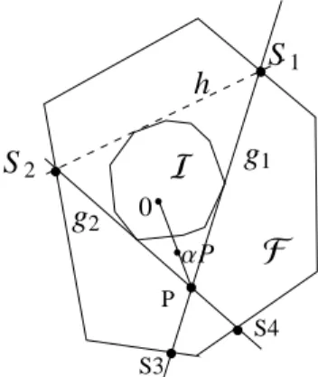
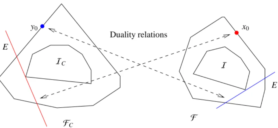
In words Cor. 3.2 is about the duality of ai, whose convex hull equalsI, and the hyperplanes E^(C)_i which underlie the construction ofF_C. The next lemma de- scribes a similar relation of points on the boundary ofFC to dual hyperplanes which are tangential to I, cf. Sec. 3 in [21]. Fig. 1 illustrates the relations.

Lemma 3.3. The point y0 ∈ R^s−1 is a boundary point ofF_C if and only if the dual affine hyperplane E to y0

is a tangential plane toI(which does not intersect the interior ofI) and at least one index i₀∈ {1, . . . ,k}exists so that ai0by (6) is a point of tangency of E toI.

Proof. First y0 ∈ F_C, that means UΣ₁

y0

≥0, is equiv- alent to

(UΣ)(:,2 : s)y0≥ −U(:,1)σ1. Equivalently it holds for all i∈ {1, . . . ,k}that

(UΣ)(i,2 : s)y0

U(i,1)σ1

≥ −1 (12) or a^T_iy0 ≥ −1 with ai by (6). Equality in (12) for one index i0, i.e. a^T_i

0y0 =−1, is equivalent to y0being located on the boundary ofF_C.

The dual affine hyperplane to y0reads by its definition E = {x ∈ R^s−1 : x^Ty0 = −1}. Hence (12) shows that all ai are located in the half-spaces on one side of the affine hyperplane E. The convex hull of the aiequals Iso that E cannot intersect the interior ofI. Finally, ai₀∈E is a point of tangency since a^T_i

0y0=−1 as shown above. This proves the two directions of the if-and-only- if conditional statement.

Lemma 3.3 can be reformulated for points on the boundary ofF which are set in relation to tangential affine hyperplanes ofI_C, see Fig. 1.

Corollary 3.4. Let x0 ∈R^s−1be located on the bound- ary ofF. Then the dual affine hyperplane E to x0 is a tangential plane toI_C. At least one index j0 ∈ {1, . . . ,n}

exists so that bj₀by (7) is a point of tangency of E toI_C. This point satisfies

V( j₀,2 : s)x₀=−V( j₀,1) or equivalently b^T_j

0x0=0.

The next step is to extend Lemma 3.3 in a way that the vertices ofF_Care shown to be the dual points of the affine hyperplanes which include facets of the polyhe- dronI. Up to now we have proved that the tangential hyperplanes touch the polygon at least in a vertex. It re- mains to show that this hyperplane contains an edge (for s= 3) or in general a facet ofI. This is the basis for computing the vertices ofFCby using the polyhedronI and also to compute the vertices ofF by usingIC.

.

H

0 y

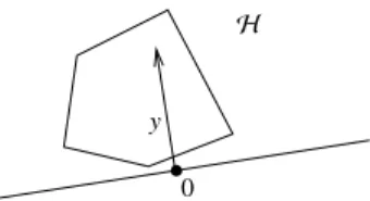
Figure 3: A convex set which does not include the origin is necessarily a subset of a half-planeHdefined by an appropriate y,0.

3.4. Duality of the facets ofIand the vertices ofF_C This section analyzes a duality of the facets ofIand the vertices ofF_C. First we show that the origin is an interior point ofI.

Lemma 3.5. Let DD^T be an irreducible matrix. Then the origin x=0 is an interior point ofI.

Proof. We assume x =0 not to be an interior point of I. Then the convexity ofIimplies thatIis a subset of the half-plane

H ={z∈R^s−1 : z^Ty≥0}

for a proper nonzero vector y∈R^s−1, see Fig. 3. Further (6) implies that

0≤a^T_iy= 1

σ1U(i,1)UΣ(i,2 : s)y, i=1, . . . ,k, which reads in vectorial form

1

σ₁diag(1/U(1,1), . . . ,1/U(k,1))UΣ(:,2 : s)y≥0.

Since σ1 > 0 and as the first singular vector U(:,1) can be assumed strictly positive (due to the Perron- Frobenius theory on the assumption of irreducibility of DD^T), the last equation proves that UΣ(:,2 : s)y ≥ 0 for the given y , 0. This contradicts Corollary 2.3 in [28] for irreducible DD^T since a nonnegative and nonzero linear combination of the columns of UΣal- ways has a nonzero contribution from the first singular vector U(:,1).

The Lemma 3.3 is needed in order to prove that the vertices of F_C and the facets of the polyhedronIare dual. Facets are nondegenerate faces of a polyhedron, i.e. the dimension of a facet is one less the dimension of the polyhedron (or mathematically a facet has the codi- mension 1). See Fig. 2 of an illustration of the content of the following theorem.

Theorem 3.6. Let D^TD and DD^T be irreducible matri- ces with D of the rank s ≥ 3. A point y₀is a vertex of FCif and only if its dual affine hyperplane E contains a facet ofI, i.e. a face of the codimension 1.

5

. .

y₀

F_C F

I_C I

E E

Duality relations

Figure 1: Lemma 3.3 describes a duality relation of a boundary point y0∈ FCto a tangential plane ofIas well as of a boundary point x0∈ Fto a tangential plane ofIC.

. .

y0

F_C F

I_C I E

E Duality relations

Figure 2: Theorem 3.6 describes a duality relation of a vertex y0 ∈ FCto a tangential plane ofIwhich encloses a facet ofI. Further a vertex x0∈ Fis dual to a tangential plane ofICwhich contains a facet ofI.

6

Proof. First we prove the direction that a facet ofIis dual to a vertex y0ofF_C. In order to show that a dual vector y₀in the sense of Def. 3.1 exists, we have to prove that the facet is enclosed by an affine hyperplane and not only by a hyperplane. (The crucial point is that Def. 3.1 with y^TzE = −1 specifies an affine hyperplane which does not include the origin.) Due to Lemma 3.5 the ori- gin 0 = (0, . . . ,0)^T ∈ R^s−1 is an interior point of I.

Hence the facet E ofIcannot contain the origin. Thus a dual vector y0 exists which represents the affine hy- perplane E in the form E ={x∈R^s−1 : y^T₀x=−1}. It remains to show that y0is a vertex ofF_C.

As E contains a facet (codimension 1) ofI, there ex- ist s−1 affine independent vertices ai₁, . . . ,ais−1 by (6) whose convex hull equals the facet. Therefore it holds that

y^T₀ai_j =−1, j=1, . . . ,s−1, (13) y^T₀aℓ≥ −1, ℓ∈ {1, . . . ,k} \ {i₁, . . . ,is−1}. (14) Thus (13) and (14) show that y₀ fulfills the condition UΣ(1,y₀)^T ≥ 0 for a membership inF_C according to (9). Furthermore from (13) it follows that y₀belongs to exactly s−1 of the affine hyperplanes which encloseF_C. For the selected indexes i1, . . . ,is−1these s−1 affine hy- perplanes are linearly independent. Hence y0is a vertex ofF_C (and not only an interior point of an edge). This completes the proof of the first direction.

In order to prove the other direction let y0be a vertex ofF_C. As y0is a vertex it holds that in s−1 components of UΣ(1,y^T₀)^T ≥ 0 equality is attained. Let i1, . . . ,is−1

be the indexes of these components. Reversing the argu- ments of the first part of the proof proves that the dual hyperplane E encloses the facet ofIwith the vertices a_i1, . . . ,a_is−1.

Analogously, this result is valid for facets ofI_C and the dual vertices ofF, see Fig. 2.

Corollary 3.7. On the assumptions of Thm. 3.6 the fol- lowing equivalence holds: A point x0is a vertex ofF if and only if its complementary affine hyperplane E con- tains a facet ofI_C.

The duality results of Thm. 3.6 enable a fast compu- tation ofF_C if the polyhedronIis known, see the fol- lowing Sec. 3.5. Additionally, the duality helps to de- termine the setsF andIeven in the presence of noise or perturbations, see the second part of this paper.

Fig. 4 illustrates the duality of the facets ofIto the vertices ofF_Cas well as the duality of the facets ofI_C to the vertices ofF. These figures have been generated for a three-component model problem which is taken

from the FACPACK-homepage, see [29] for the details.

Related pairs of objects (vertices and edges of the poly- gons) are marked by the same, continuously changing color. Additionally, Fig. 5 illustrates these relations for a four-component model problem. Vertices of the three- dimensional polyhedrons are dual to the 2D-facets of the dual polyhedra.

3.5. Fast computation ofF andF_C

The setsF andIare decisive ingredients for the ge- ometric construction ofM, see [16, 5, 23, 11, 12]. The same geometric construction algorithm applied to F_C andI_C leads to the AFSM_Cfor the concentration fac- tor. The setsF andFC are intersections of the n, re- spectively k, affine hyperplanes (10) and (11) which are oriented each in a way that they include the origin. Our approach for the fast computation of the four polyhedra F,I,F_CandI_Ccan significantly decrease the compu- tation times forMandM_C.

This section introduces a direct and also an indirect approach for the computations ofF andF_C. These ap- proaches are based on Thm. 3.6 and Cor. 3.7. A compar- ison of these techniques for a three-component model problem is contained in Sec. 5.2. The following two subsections focus onF; everything can easily be refor- mulated forF_C.

3.5.1. Direct computation ofF

A direct and intuitive approach to compute the poly- hedron F is as follows: Initially s affine half-spaces are selected in a way that their intersection is bounded.

Then all other affine half-spaces (which finally tightly encloseF) are analyzed whether or not a further reduc- tion of the current intersection can be gained. If so, then the new smaller intersection is the new approximation toF. This iteration terminates inF. See also the ap- proach in [23].

3.5.2. Indirect computation ofF

The polyhedronF can also be computed in an in- direct way as already suggested by Beyramysoltan et al. [3], see Sec. 3. The formal mathematical justifica- tion (which requires the irreducibility of the matrices D^TD and DD^T) is given in Thm. 3.6 and Cor. 3.7. Fol- lowing [3], firstI_Cis computed by simply forming the convex hull of the vectors b_j, see Eq. (9). MatLabpro- vides for this the routineconvhull. In a second step for each facet ofICits dual vertex ofF is computed.

7

0 2 4 6 8

−10

−5 0 5

y₁ y2

Vertices ofFCand the facets ofIC

−0.5 0 0.5 1 1.5

−1

−0.5 0 0.5 1

x1

x2

Vertices ofF and the facets ofI

Figure 4: The duality of the facets ofIand the vertices ofFCand also the duality of the facets ofICand the vertices ofFis illustrated for the three-component model problem from [29]. Left: The setsIC,FCas well as the three isolated subsets of the AFSMC(in gray) are shown. Right:

The setsI,F as well as the three isolated subsets of the AFSM(in gray) are shown. The series of dotted lines encloses and defines the convex setFC(left) respectivelyF (right); the boundaries of these two sets are drawn by black solid lines. The dual pairs of facets ofICand vertices of Fare each plotted by using the same color. Analogously, the same colors are used for the dual pairs of facets ofIand vertices ofFC.

−5 0

5

−5 0 5

−10

−5 0 5 10

y1

y2

y3

Vertices ofFCand the facets ofIC

−0.4 −0.2 0 0.2 0.4

−0.4

−0.2 0 0.2 0.4

−0.5 0 0.5

x₁ x2

x3

Vertices ofF and the facets ofI

Figure 5: The duality of the facets ofIand the vertices ofFCand also the duality of the facets ofICand the vertices ofF are illustrated for a four-component model problem. Left: The setsICandFCare shown. Right: The setsIandFare drawn. The edges of the polyhedraFCandF are plotted by black lines. The dual pairs of facets ofI_Cand vertices ofF are plotted by using the same color. Analogously, the same colors are used for dual pairs of facets ofIand vertices ofF_C.

8

4. Simultaneous computation of M and M_C for three-component systems

In 1985 Borgen and Kowalski [5] introduced the ge- ometric construction of the AFS for three-component systems (s=3) on the basis of results gained in [13, 16].

The method was revitalized by Rajk ´o [23] in 2005 and has been extended in [11, 12]. The idea of the geo- metric construction is to form the inner boundary ofM by means of all triangles which enclose INNPOL and which are enclosed by FIRPOL (F). In combination with the polygon F, which is a superset of the AFS M, this yields the boundary of the AFS. This boundary comprises of separate closed curves if the AFS consists of isolated subsets. We call these subsets the segments of the AFS.

In contrast to the numerical AFS approximation by means of solving optimization problems, the benefit of a geometric construction of the AFS is that the inner boundary points of the AFS can be constructed exactly.

However, the boundary of the AFS is in general not a polygon, but consists of a sequence of smooth curves which are joined to a continuous boundary curve. The construction of the smooth boundary curves requires a discretization of the problem and results in approxima- tion errors and also in the unavoidable small rounding errors by the computer arithmetic. The computational costs for the geometric construction are relatively low.

Furthermore, degenerated segments of the AFS, namely points or line segments, can also be computed precisely (aside from the small numerical rounding errors). Bor- gen plots are ideal tools for the investigation of theoret- ical questions on noise-free and non-perturbed model data. For experimental noisy data some modifications of the Borgen plot construction are required. In [11, 12]

an extended construction algorithm has been presented which can deal with small perturbations. Nevertheless, the purely numerical methods in [2, 7, 27] are still more robust for AFS computations for experimental spectral data.

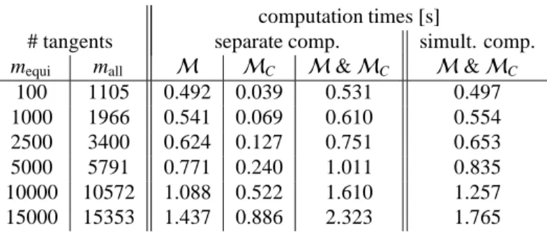
This section presents a new method for the simulta- neous geometric construction of the spectral AFS and also the AFS for the concentration factor. The new con- struction algorithm can form the two AFS sets at costs which are slightly higher than the costs for construct- ing only one AFS set by the classical algorithm. This is a considerable improvement on the classical approach with double costs if the two AFS setsM andM_C are constructed in separate steps.

In this section we first define inner boundary points and prove a certain property of these points. The clas- sical Borgen plot construction is briefly reviewed and

.

P

. .

. . .

S3

S4

. .

F I ^g

g

S

S

h

0 αP

Figure 6: Construction of inner boundary points by triangles tightly includingIwith the vertices S1and S2on the boundary ofFand a third vertex inF.

the new simultaneous construction is explained. The suggested method is tested for a model problem whose AFS consists of an isolated point, a line segment and a bounded planar segment.

4.1. Inner boundary points

The following definition of an inner boundary point refers to the ray casting concept for AFS computations as suggested in [31]. The definition is not limited to the case s=3.

Definition 4.1. A point x∈ Mis called an inner bound- ary point ifγx<Mfor allγ∈(0,1). In words x is the only member ofMon the line segment from the origin 0 to x. A point x∈ Mis called an outer boundary point ifγx<Mfor allγ >1.

A direct consequence of these definitions is summa- rized in the next remark.

Remark 4.2. A point x ∈ Mcan belong to the inner and to the outer boundary according to Def. 4.1. Special examples are punctiform or line-shaped AFS segments.

The key idea of the geometric construction of the AFS for three-component systems [16, 5, 23, 11] is that the inner boundary points are constructed by certain tri- angles. Each of these triangles is a triangle which tightly includesI, is contained inF and has two of its vertices on the boundary ofF. Then the third vertex is an in- ner boundary point. This property is proved in the next lemma.

Lemma 4.3. For s=3 let h be a tangent ofI. The two points of intersection of h with the boundary ofF are S₁ and S2, see Fig. 6. Let g1be a further tangent ofIwhich runs through S1 and g2 be another tangent ofIwhich 9

runs through S2so that h, g1and g2tightly encloseI.

The point of intersection of g1and g2is denoted by P.

If P∈ F, then P is an inner boundary point ofM.

Proof. We consider the case that P∈ F. Then the tri- angle construction guarantees that P∈ M, see [5]. We assume P not to be an inner boundary point ofMand derive a contradiction. If P is not an inner boundary point, then anαwith 0 < α < 1 exists so thatαP is closer to the origin and is still an element ofM, see Fig. 6. AsαP is a feasible point, two other points S^′ and S^′′ exist inF so that the triangle∆^′with the ver- ticesαP, S^′and S^′′includesIand is contained inF. The geometry in the AFS plane, see Fig. 6, shows (by considering tangents ofIwhich run throughαP) that P, S^′and S^′′are on the same side of h. Moreover, S^′and S^′′are not located on h asIis a convex set with a pos- itive volume (since the origin is an interior point ofI).

Thus the line segment S^′-to-S^′′which is an edge of∆^′ must intersectI. This is a contradiction to∆^′including I.

4.2. Classical Borgen plots

The tangent-rotation method for the geometric con- struction of the AFS for three-component systems is ex- plained, e.g., in [5, 23, 11, 12]. The basic idea is to ro- tate a tangent h around the polygonI. For each tangent an inner boundary point P is constructed in the way as explained in Lemma 4.3. In a computer implementation the rotation of the tangent is discretized by considering only a fixed number of equiangular tangents. In order to find all critical boundary points, one also considers all tangents which coincide with a facet ofIand also the families of possible tangent lines at vertices ofI.

In order to detect line-shaped (1D) AFS segments addi- tional tangents are to be analyzed. This process results in a finite set of points which discretizes the boundary curve of the inner boundary. The outer boundary ofM coincides with a subset of the boundary ofF. The spa- tial resolution of the inner boundary increases with a decreasing finite rotation angle of the tangent. In the generalized Borgen plot module of FACPACK [29] we typically use 3600 equiangular tangents in order to at- tain a sufficiently resolved boundary ofM.

4.3. Simultaneous Borgen plots

The standard approach to compute the Borgen plot for the concentration factor is to apply the algorithm to the transposed data matrix D^T. This doubles the costs for the construction ofMandM_C compared to a con- struction of onlyM. The simultaneous construction of the dual Borgen plots determines the inner boundary of

M_C as a by-product of the construction of the spectral AFSM. In contrast to the classical Borgen plots each tangent h is not only used to construct a single trian- gle, but three of them. In terms of the notation used in Lemma 4.3 these two additional triangles result in the two points Q and R which are possible candidates for inner boundary points ofMC.

4.3.1. Construction of the inner boundary ofM_C We continue with the notation from the proof of Lemma 4.3, see Fig. 6. Let∆be the triangle with the vertices P, S1 and S2. Furthermore, let S3be the sec- ond point intersection of g1 with the boundary ofF in a way that S3,S1. Based on this construction the dual point of the line through S2and S3 is an inner bound- ary point of M_C provided that this point is located in F_C. This is proved next in Thm. 4.4. Furthermore it is possible to compute a second auxiliary triangle with the vertices S₁, S₂and S₄where S₄is the second point of intersection of g₂and the boundary ofF with S₄,S₂. Then the dual point of the line through S1and S4is an inner boundary point ofMC provided that the point is located inFC.

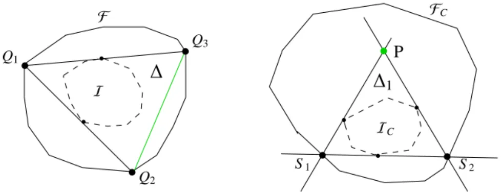
Theorem 4.4. Let the three points Q₁, Q₂ and Q₃ be located on the boundary ofF and span the triangle∆, see Fig. 7. The triangle∆is assumed to includeI. Let the two edges through Q1be tangential toI. Further, let

∆1 be the triangle which is spanned by the dual points of the edges of∆in the sense of Lem. 3.3. (Equivalently the three edges of∆1are dual to either Q1, Q2or Q3.)

Then the triangle∆1fulfills the conditions of Lemma 4.3 and the point P which is dual to the line through Q2

and Q3is an inner boundary point ofMCprovided that P is contained inF_C.

Proof. Cor. 3.4 guarantees that the three straight lines which are dual to Q₁, Q₂and Q₃ are tangential toI_C. These lines form a triangle∆₁ (as∆defines a feasible nonnegative factorization D = CS^T with∆₁ being re- lated to C). See Fig. 7 for the geometry. Two of the edges of∆are tangential toI. Hence Lemma 3.3 proves that two vertices of ∆1 are located on the boundary of FC. Thus Lemma 4.3 applies to the triangle ∆1 with the vertices S1, S2 and P and proves that P is an inner boundary point ofM_Cprovided that P∈ F_C. This point P is the dual point of the straight line through Q2 and Q3, see the green line and point in Fig. 7.

Theorem 4.4 is the basis for the simultaneous Borgen plot algorithm which is explained next.

10

. .

.

.

. . ^{. .} .

.

. P

Q₁

Q2

Q3

S1 S2

∆ ∆

F_C F

I

I_C

Figure 7: Simultaneous construction of points P on the inner boundary ofMC, see Thm. 4.4.

−0.5 0 0.5 1 1.5 2

−1

−0.5 0 0.5 1

x1

x2

h

g1

g2

g₃

g4

S1

S₂

S₃

S₄ P

Simultaneous geometric construction inM

0 2 4 6 8

−10

−8

−6

−4

−2 0 2 4 6

y1

y2

New dual inner boundary points inM_C

Figure 8: Demonstration of the extension of the classical Borgen plots in order to compute simultaneously an inner boundary point ofMand two inner boundary points ofMCfor the three-component model problem. Left: Geometric construction of an inner boundary point. For the tangent h (broken black line) the points of intersection S1and S2(×) with the boundary ofF as well as the tangents g1and g2(black solid lines) toIare constructed. The point of intersection of g1and g2is the inner boundary point P (###). The points S3and S4are the points of intersection of g1

respectively g2with the boundary ofF. The triangles with the vertices S1, S2and S3respectively S1, S2and S4fulfill the condition of Thm. 4.4.

The dual point of g3(blue line) is contained in the dual plane which containsFCand is an inner boundary point ofMC(###in the right subplot).

Also the dual point of g4(red line) belongs toFCand so it is an inner boundary point ofMC(###in the right plot). The resulting AFS setsMand MCare plotted as gray areas. The boundaries of the supersetsFandFCare the black closed curves. The boundaries of the inner polygonsIand I_Care plotted gray.

11

4.3.2. The algorithm

The construction of the inner boundary points of the AFS M_C is embedded into the classical Borgen plot construction of the inner boundary points of the AFS M. The only step which is basically different from the classical Borgen construction is that the computed inner boundary points ofM_C require a specific ordering. To this end we use polar coordinates.

The construction of the two inner boundary points ofMC is based on Theorem 4.4. Only those points which belong to the supersetF_C successfully pass the construction. The starting point is a tangent h ofI.

1. The two points of intersection S1and S2of the tan- gent h ofIwith the boundary ofF are constructed.

2. A first tangent g1ofIthrough S1with g1 ,h and a second tangent g2ofIthrough S2 with g2 ,h are constructed.

3. The intersection of g1 and g2 is P. According to Lemma 4.3 P is an inner boundary point as far as P∈ F.

4. Additionally, the point of intersection S₃of g₁with the boundary of F is determined (in a way that S₃ , S₁) and also the point of intersection S₄ of g2 with the boundary of F is computed (so that S4 ,S2).

5. Then g3is the straight line through S2and S3. Fur- ther, g4is the straight line through S1and S4. Ac- cording to Theorem 4.4 the dual point of g3 is an inner boundary point ofM_C if it is contained in F_C. Also the dual point of g4is an inner boundary point ofM_Cif it is inF_C.

Remark 4.5. The point which is dual to g3is contained in the supersetF_C(and so it is an inner boundary point ofM_C) if and only if P is contained inF (so that P is an inner boundary point ofM). An analogous statement holds for the point which is dual to g4.

The complete algorithm is based on the rotation of the tangent h aroundI. Practically, only a fixed num- ber of m equiangular tangent lines are considered to- gether with certain additional points which serve to de- tect punctiform or line-shaped AFS segments. At the end all constructed boundary points of the AFSM_Care ordered with respect to their polar coordinates. This ap- proach is justified by the gap-free intersection property of the AFS sets [31]; this property says that the intersec- tion of an AFS with an infinite ray starting at the origin is either empty or a line-segment (which may be degen- erated to a single point).

4.3.3. Visualization of the geometric construction Fig. 8 illustrates the simultaneous Borgen plots for a three-component model problem. For a fixed tangent h of Ishows the construction of one inner boundary point ofMand two inner boundary points ofM_C. First the triangle of the classical Borgen plot yields an inner boundary point P. Then two additional triangles with the vertices S1, S2 and S3 respectively S1, S2 and S4

are formed. Finally, the dual points of g₃respectively g₄are plotted in the AFSM_C for factor C. These two points are inner boundary points ofM_C (if located in F_C.

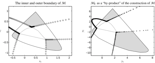
Further, Fig. 9 shows the results of the simultaneous Borgen plot algorithm. The sequences of points on the inner boundaries ofMandMCare presented for a (rel- atively small) number of m=500 tangents toI. How- ever, m=500 leads to a sufficient spatial resolution for a graphical demonstration of the principles of simulta- neous Borgen plots. The spatial resolution of the bound- ary ofM_Cis twice as high as forMsince two boundary points ofM_Ccorrespond to one boundary point ofM.

4.4. Detection of line segments and isolated points An AFS can have various shapes. The AFS can either be a topologically connected set with a hole around the origin or can consist of several isolated subsets (the seg- ments). For three-component systems (s=3) the num- ber of segments can be 1 or a multiple of 3. IfMcon- sists of three or more segments, then one segment can equal an isolated point or it can be a one-dimensional line segment. Such degenerated segments can be ob- served for properly designed model data. The (simulta- neous) Borgen plot algorithm can detect such degener- ated AFS segments.

Next we demonstrate for D=













1 1 1

0 1 1

0 0 1













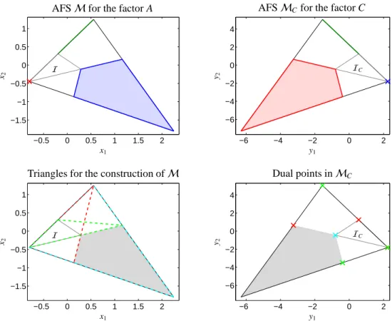
(15) that the simultaneous Borgen plot algorithm can find punctiform and line-shaped AFS segments as parts of M_C, see the upper row of plots in Fig. 10. There is no necessity to demonstrate that these degenerated seg- ments can correctly be detected in the spectral AFSM as the simultaneous Borgen plot algorithm for the first AFS coincides with the classical Borgen plot construc- tion from [5, 23, 11]; classical Borgen plots are well- known to construct degenerated AFS segments cor- rectly.

The lower two subplots of Fig. 10 explain the trian- gle and point selection. The red and the green trian- gle (broken lines) are related to the line-shaped segment 12

−0.5 0 0.5 1 1.5 2

−1

−0.5 0 0.5 1

x1

x2

The inner and outer boundary ofM

0 2 4 6 8

−10

−8

−6

−4

−2 0 2 4 6

y1

y2

M_Cas a “by-product” of the construction ofM

Figure 9: Simultaneous construction ofMandMCby the algorithm from Sec. 4.3.2. A number of m=500 equiangular tangents h has been used for the computation of the inner boundary points ofM. The steps 4 and 5 of the algorithm supply the by-product of the inner boundary points of MC. Left: The combination of the (outer) boundary ofF(closed black curve) and the results for the inner boundary points (###) ofMleads to the three isolated subsets ofM(in gray). Right: The inner boundary (×) ofM_Cis a by-product of the geometric construction forM. Together with boundaryFC(closed black curve) this makes it possible to compute the three isolated subsets of the AFSMCfor the concentration factor (gray areas).

and also two critical points of the 2D-area segment of the AFSM. These two triangles are important for the classical Borgen plots. All vertices of these two trian- gles are located on the boundary ofFand all their edges are tangents ofI. Hence each edge of the two triangles yields a dual inner boundary point ofM_C, see Thm. 4.4.

These dual points are plotted in the lower right subplot.

All points are significant (but two of them coincide) for the construction of the segments ofM_C. The last point (in cyan), which is significant for the construction of the inner boundary ofM_C, is the dual point of the cyan triangle (broken line) in the lower left plot. This tri- angle is part of the combined geometric construction.

All other points on the inner boundary ofMC, which arise from the other tangents, do not influence the final result. Hence the simultaneous geometric construction leads toMCas a by-product of the computation ofM even for this problem with degenerated punctiform and line-shaped AFS segments.

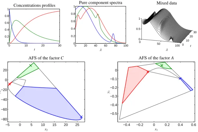
5. Numerical results and computation times This section demonstrates the effectiveness of si- multaneous Borgen plots for a three-component model problem, see Sec. 5.1. We consider various discretiza- tions of the model problem with increasing matrix di- mensions. The underlying pure component spectra, the concentration profiles and the kinetic equations are al- ways the same. The focus of the comparative analy- sis is on the computation times. These times are com-

pared with some well-established methods. Simultane- ous Borgen plots have at least the same precision (spa- tial resolution) as the classical geometric constructive Borgen plots.

We start with the construction and computation ofF andIand their counterpartsI_C andF_C. We compare the proposed indirect computation ofF, see Sec. 3, with the direct approach and also with the numerical approxi- mation by means of the polygon inflation method. Then the simultaneous Borgen plot construction is compared with two separate runs of the classical Borgen plot con- struction. Finally, simultaneous Borgen plots are com- pared with the FACPACK implementations of the poly- gon inflation method [27, 28] and with the generalized Borgen plots [11, 12].

We run all computations on a single core of a 3.40GHz Intel CPU of a standard personal computer with 16GB RAM. The major part of the program is writ- ten in C; however some MatLabroutines, e.g. the rou- tineconvhull, have been used.

5.1. The three-component model problem

We consider the first-order consecutive reaction scheme

X−→^k1 Y −^k→² Z

with k1 = 0.5 and k2 = 0.1 and the initial concen- trations cX(0) = 1 and cY(0) = cZ(0) = 0. The 13