Performance of Top Quark and W Boson Tagging in Run 2 with ATLAS

ATLAS-CONF-2017-064 14/02/2018

ATLAS Note

ATLAS-CONF-2017-064

14th February 2018

Performance of Top Quark and W Boson Tagging in Run 2 with ATLAS

The ATLAS Collaboration

A problem affecting Figures 16a, 16b, 18a, 18b, 19a, 19b, 28a, 28b, 35a, 35b was found. The document was therefore revised with corrected figures on February 14, 2018.

The performance of hadronically-decaying top-quark and W -boson taggers in pp collisions at

√ s = 13 TeV recorded by the ATLAS experiment at the Large Hadron Collider is presented.

A set of techniques, including some new to the data recorded in 2015 and 2016, are studied to determine a set of optimal cut-based taggers for use in physics analyses. A further extension is made to study the utility of combinations of substructure observables as a multivariate tagger using boosted decision trees and deep neural networks in comparison with taggers based on two-variable combinations. The performance of these taggers is studied with the data collected during 2015 and 2016 in t¯ t , dijet and γ + jet event topologies.

© 2018 CERN for the benefit of the ATLAS Collaboration.

Reproduction of this article or parts of it is allowed as specified in the CC-BY-4.0 license.

1 Introduction

With the increase to 13 TeV center-of-mass energy in Run 2 of the Large Hadron Collider (LHC) [1], it is increasingly important for searches for physics beyond the Standard Model to probe processes involving highly boosted massive particles, such as W bosons and top quarks, with recent examples from ATLAS in Refs. [2–5].

To fully exploit these final states, reconstructing the hadronic decay modes of these massive particles is of great importance. The identification of the origin of a hadronic jet can be used as an effective tool to reject events produced by background processes and improve the sensitivity in searches for physics beyond the Standard Model.

For W -boson and top-quark jet identification, physically motivated observables exploiting the radiation pattern within the jet have been used to effectively tag large-radius jets [6–10]. This work is intended to expand upon those studies and provide a more comprehensive investigation of tagging techniques applicable to the identification of both W bosons and top quarks.

The contents of this note are organized as follows: Section 2 briefly describes the ATLAS detector, followed by Section 3 with a description of the Monte Carlo and data samples used in the analysis.

The set of substructure techniques investigated here is described in Section 4 where a signal definition based on the parton decay products is also introduced. The optimization procedure used to determine the optimal tagger for use in searches following this signal definition and new inputs is described in Section 5. Additionally, comparisons are made of W -boson and top-quark identification techniques using simulated data at

√ s = 13 TeV. In Section 6, the data recorded in 2015 and 2016 is used to investigate the

performance of these tagging techniques by measuring signal and background efficiencies using boosted

lepton+jet t¯ t , dijet and γ + jet topologies. Concluding remarks are given in Section 7.

2 ATLAS detector

The ATLAS detector [11] at the LHC covers nearly the entire solid angle around the collision point. It consists of an inner tracking detector (ID) surrounded by a thin superconducting solenoid, electromagnetic and hadronic calorimetry, and a muon spectrometer composed of three large superconducting toroid magnets. For this study, important subsystems are the calorimeters, which cover the pseudorapidity range

1

|η| < 4.9. Within the region |η | < 3.2, electromagnetic calorimetry is provided by barrel and endcap high- granularity lead/liquid-argon (LAr) electromagnetic calorimeters, with an additional thin LAr presampler covering |η| < 1.8 to correct for energy loss in material upstream of the calorimeters. Hadronic calorimetry is provided by a steel/scintillating-tile calorimeter, segmented into three barrel structures within |η | < 1.7, and two copper/LAr hadronic endcap calorimeters. The forward region 3.2 < |η | < 4.9 is instrumented with copper/LAr and tungsten/LAr calorimeter modules. Inside the calorimeters, there is a 2 T solenoid magnet that surrounds the inner tracking detector which measures charged-particle trajectories covering a pseudorapidity range |η| < 2.5 with pixel and silicon microstrip detectors (SCT), and additionally covering the region |η | < 2.0 with a straw-tube transition radiation tracker (TRT).

The muon spectrometer (MS) comprises separate trigger and high-precision tracking chambers measuring the deflection of muons in a magnetic field generated by superconducting air-core toroids. The precision chamber system covers the region |η | < 2.7 with three layers of monitored drift tubes, complemented by cathode strip chambers in the forward region where the background is highest. The muon trigger system covers the range |η| < 2.4 with resistive plate chambers in the barrel and thin gap chambers in the endcap regions. A two-level trigger system is used to select events for offline analysis [12]. The first pass, named the level-1 trigger, is implemented in hardware and uses a subset of detector information to reduce the event rate to 100 kHz. This is followed by a software-based high-level trigger which reduces the final event rate to less than 1 kHz.

1ATLAS uses a right-handed coordinate system with its origin at the nominal interaction point (IP) in the centre of the detector and thez-axis along the beam pipe. The x-axis points from the IP to the centre of the LHC ring, and the y-axis points upwards. Cylindrical coordinates (r, φ) are used in the transverse plane,φ being the azimuth’s angle around thez-axis.

The pseudo-rapidity is defined in terms of the polar angleθasη=−ln tan(θ/2). Angular distance is measured in units of

∆R≡

q(∆η)²+(∆φ)².

3 Samples

The taggers described in this note are studied using three Monte Carlo (MC) samples for signal and background processes. The dijet process is used to simulate jets from gluons and other (non-top) quarks and this process is modelled using the Pythia8 (v8.186) [13] generator with the NNPDF2.3LO [14]

parton distribution function (PDF) set and the A14 tune [15]. Events are generated in slices of jet p

to sufficiently populate the kinematic region of interest. Event-by-event weights are applied to correct for this generation and to produce the expected smoothly-falling p

distribution expected for multijet background.

The signal samples containing either high- p

top-quark or W -boson jets are obtained from two physics processes modelling phenomena beyond the Standard Model. For the W -boson sample, the high-mass W

→ W Z → qqqq is used. For the top-quark sample, high-mass Z

→ t¯ t events are used as a source of signal jets. Both the W bosons and top quarks are required to decay hadronically. The two signal processes are simulated using the Pythia8 generator with the NNPDF2.3LO PDF set and A14 tune for multiple values of the resonance ( W

or Z

boson) mass between 400 and 5000 GeV in order to populate the entire p

range

from 200 to 2500 GeV and to ensure that the calculated signal efficiencies have small statistical uncertainties.

For the study of W -boson and top-quark jets in data, described in Section 6, a number of Monte Carlo samples are needed to model both the t¯ t signal and backgrounds. The Powheg-Box v2 generator [16]

is used to simulate t t ¯ and single-top-quark production in the W t - and s -channels, while for the single- top-quark t -channel process, Powheg-Box v1 generator is used. The matrix-element generation in Powheg-Box is interfaced to the CT10 [17] NLO PDF set. For all processes involving top quarks, the parton shower, fragmentation, and the underlying event are simulated using Pythia6 (v6.428) [18] with the CTEQ6L1 [19] PDF set and the corresponding Perugia 2012 tune (P2012) [20]. The top-quark mass is set to 172.5 GeV. The h

parameter, which controls the p

of the first additional emission beyond the Born configuration, is set to the mass of the top quark. The t t ¯ process is normalized to the cross- sections predicted to next-to-next-to-leading-order (NNLO) in α

and next-to-next-to-leading logarithm in soft-gluon terms while the single-top-quark processes are normalized to the NNLO cross-section predictions.

Several additional variations of the t¯ t generator are used for the estimation of modeling uncertainties.

Estimates for the parton-showering and hadronization modelling uncertainty are derived by comparing results with the Powheg-Box v2 generator in tandem with Herwig++ (v2.7.1) [21] instead of Pythia6. To estimate the hard-scattering-modelling uncertainty, the MadGraph5_aMC@NLO (v2.2.1) generator [22]

(hereafter referred to as MC@NLO) with Pythia6 is used. To estimate the uncertainty on modelling of additional radiation, the Powheg-Box v2 generator with Pythia6 is used with modified renormalization and factorization scales (both × 2 or × 0 . 5) and simultaneously modified h

parameter ( h

= m

or h

= 2 × m

).

Samples of W/Z +jets and Standard Model diboson ( W W / W Z / Z Z ) production are generated with final states that include either one or two charged leptons. The Sherpa [23] generator version 2.1.1 and version 2.2.1 are used with the CT10 PDF set to simulate the diboson production and W/ Z +jets processes, respectively. The W/Z +jets events are normalised to the NNLO cross sections.

2As the combination of these signal samples with different generated heavy resonance masses results in irregular top-quark and W-bosonp_Tdistributions, the events are reweighted on the generator level to either a flat or a QCD background-like falling p_Tdistribution in the following.

For the study of γ + jets in data, events containing a photon with associated jets are simulated using the Sherpa 2.1.1 [23] generator, requiring a photon transverse momentum above 140 GeV. Matrix elements are calculated with up to 4 partons at LO and merged with the Sherpa parton shower [24] using the ME+PS@LO prescription [25]. The CT10 PDF set is used in conjunction with dedicated parton shower tuning developed by the Sherpa authors.

The Monte Carlo samples are processed through the full ATLAS detector simulation [26] based on Geant4 [27]. Additional simulated proton–proton collisions generated using Pythia8 (v8.186) with the A2 [28] tune and MSTW2008LO PDF set [29] are overlaid to simulate the effects of additional collisions from the same and nearby bunch crossings (pile-up), with a mean number of 24 collisions per bunch crossing. All simulated events are then processed using the same reconstruction algorithms and analysis chain as is used for real data.

Data are collected in three broad categories to study the signal and the background. For the signal, a set of observed top-quark and W -boson candidates is obtained from a sample of t¯ t candidates in which one top quark decays semi-leptonically and the other decays hadronically, the so-called lepton plus jets decay signature. The background is studied using data samples of dijet events and γ + jet events. In addition to covering different p

regions, the dijet and γ + jet samples differ in what partons initiated the jets under study. In the γ + jet topology the jets are dominantly initiated by quarks over the full p

range studied, while for the dijet topology the fraction of quarks initiating the jets is slightly smaller than the gluon fraction at low p

and becomes large at high p

. The data for the t¯ t and γ + jets studies were collected during normal operations of the detector and correspond to an integrated luminosity of 36 . 1 fb

. For the dijet analysis additional data where the toroid magnet was turned off can be used, resulting in 36 . 7 fb

in total.

The signal lepton plus jets events are collected with a set of single-electron and single-muon triggers that become fully efficient for p

of the reconstructed lepton greater than 28 GeV. The dijet events are triggered by a single large- R jet trigger that becomes fully efficient for an offline-jet p

of approximately 450 GeV.

Additionally for the dijet studies, small contributions from signal processes are accounted for with the

use of the simulated Standard Model W/Z plus jets and all-hadronic t¯ t samples. The γ + jet events are

triggered by a single-photon trigger that becomes fully efficient for an offline-photon p

of approximately

155 GeV. Additionally, for the γ + jet studies the small contributions from signal processes are accounted

for with the use of the simulated W/Z + γ and t¯ t + γ samples.

4 Jet substructure techniques

The reconstruction and identification of hadronic decays of boosted W bosons and top quarks can broadly be divided into two stages, grooming and tagging. A number of techniques and observables pertaining to these two categories have been described and investigated extensively in previous work [8, 9] with only a short summary of the relevant techniques presented here.

4.1 Jet reconstruction and grooming

Jets within ATLAS are reconstructed from noise-suppressed topological clusters [30] that are individually calibrated to correct for effects such as the non-compensation of the calorimeter response and inactive material [31]. The clusters are set to be massless. They form the basis for the set of constituents from which large- R jets are reconstructed using the anti- k

algorithm [32] with a radius of R = 1 . 0 and further trimmed to remove the effects of pile-up and underlying event. Trimming [33] is a grooming technique in which the original constituents of the jets are reclustered using the k

algorithm [34] with a distance parameter R

in order to produce a collection of subjets. These subjets are then discarded if they carry less then a specific fraction ( f

) of the p

of the original jet. The trimming parameters used here are R

= 0.2 and f

= 5%. These jets are then calibrated in a two-step procedure that first corrects the jet energy scale and then the jet mass scale [31, 35].

The resultant set of constituents forms the basis from which further observables are calculated. The notable exceptions are the inputs for the shower deconstruction [36] and the HEPTopTagger [37, 38] algorithms, described later in more detail, that make use of the Cambridge/Aachen (C/A) jet algorithm [39, 40].

For the purpose of identifying the flavor of the jet at truth level in Monte Carlo events, a second set of jets is formed from truth particles with lifetimes greater than 10 picoseconds, except for muons and neutrinos which are not included. These jets are reconstructed with the anti- k

algorithm with a distance parameter of R = 1 . 0 but are not modified with the trimming algorithm. These jets are referred to as truth jets and the related quantities such as the p

of the jets are referred to as p

T

.

In the MC-simulation-based study presented in Section 5, the event selection isolates ensembles of jets which are representative of those originating from either W bosons or top quarks (signal) and gluon or other quarks

(background). Initially, events which contain a reconstructed primary vertex with at least two tracks are selected. In each event the two highest- p

truth jets are retained if they satisfy | η| < 2 and have a p

greater than 200 GeV in the case of the W -boson or background quark and gluon jets, and greater than 350 GeV for top-quark jets. The retained truth jets and the reconstructed jets that are truth-matched to those as described below are used.

It is important to note that the tagging techniques used to identify signal W -boson or top-quark jets are typically designed under the hypothesis of a signal model for the jets. In the study presented in Section 5, signal jets are defined as hadronically-decaying W bosons or top quarks when all partonic decay products are fully contained within the region of interest of the reconstructed jet in a three-step process. First, reconstructed jets are matched to truth jets. Next, those truth jets are matched to truth W bosons and top quarks ( W , t ). Lastly their partonic decay products (two light quarks for hadronically-decaying W bosons and an additional b quark for top quarks decaying into a W boson and a b quark) are matched to the initial reconstructed jet. All stages of this matching procedure are performed with simple matching in ( η , φ )

3 This includes quark flavours other than top quarks.

with ∆R < 0 . 75

. In particular, the containment depends strongly on the p

of the particle, as shown in Figure 1.

[GeV]

Truth WBoson pT

0 200 400 600 800 1000 1200 1400

W Boson Jet Containment Fraction

0 0.2 0.4 0.6 0.8 1 1.2

1.4 ^WJet Contains

and q2

q1

or q2

only q1

ATLAS

Simulation Preliminary q2

q1

truth W→

R=1.0 truth jets anti-kt

| < 2 ηjet

|

[GeV]

Truth Top Quark pT

0 200 400 600 800 1000 1200 1400

Top Quark Jet Containment Fraction

0 0.2 0.4 0.6 0.8 1 1.2

1.4 Top Jet Contains

and q2

b and q1

or q2

b and only q1

and q2

only q1

only b ATLAS

Simulation Preliminary q2

b q1

truth t →

R=1.0 truth jets anti-kt

| < 2 ηjet

|

Figure 1: Containment of theW boson and top quark decay products in a single truth level anti-ktR=1.0 jet as a function of the particle’s transverse momentum.

4.2 Jet mass

The jet mass provides the most powerful single discriminant and is typically constructed purely from the topocluster constituents of the jet. However, at extremely high p

, it becomes advantageous to use the spatial granularity of tracks reconstructed in the inner detector to construct an observable called the track-assisted jet mass ( m

), defined as

m

= m

× p

T

p

T

(1) in which m

and p

T

are the invariant mass and p

calculated from tracks associated with the large- R trimmed calorimeter jet and p

T

is the p

of the original trimmed large- R jet.

In order to take full advantage of this new observable and the calorimeter-based jet mass, a new combined mass ( m

) definition uses a linear combination of the two. The variables combined in a weighted average. The assigned weight w

for the track-assisted mass is defined as

w

= σ

TA

σ

calo

+ σ

TA

(2) where σ

and σ

are the m

and calorimeter mass resolutions, respectively. The calorimeter weight, w

= 1 − w

, is defined so that the sum of both weights equals unity. An illustration of the m

distribution for signal and background events is shown in Figure 2. Further details can be found in Ref. [35].

4For R = 1.5 C/A jets the containment cuts are increased to 0.75·1.5=1.125.

Combined Mass [GeV]

0 50 100 150 200 250 300

Normalized amplitude / 3 [GeV]

0 0.02 0.04 0.06 0.08 0.1 0.12 0.14 0.16

0.18 ^ATLAS Simulation Preliminary = 13 TeV

s

R=1.0 jets anti-kt

= 0.2) = 0.05 Rsub

Trimmed (fcut

= [200, 500] GeV

truth

pT

| < 2

truth

|η Jets W Dijets Top Jets

Combined Mass [GeV]

0 50 100 150 200 250 300

Normalized amplitude / 3 [GeV]

0 0.02 0.04 0.06 0.08 0.1 0.12 0.14 0.16 0.18

ATLAS Simulation Preliminary = 13 TeV

s

R=1.0 jets anti-kt

= 0.2) = 0.05 Rsub

Trimmed (fcut

= [1000, 1500] GeV

truth

pT

| < 2

truth

|η Jets W Dijets Top Jets

Figure 2: Distributions of the combined track-assisted + calorimeter jet mass for lowp_T[200-500 GeV] (left) and highp_T[1000-1500 GeV] (right)W, top and QCD jets.

4.3 Tagging techniques

In addition to the jet mass, a number of observables and techniques can be used to further identify a jet as originating from a W boson or a top quark.

4.3.1 Jet moments

The first broad class of observables are those referred to as jet moments or simply jet substructure variables that are analytically defined and that quantify the nature of the radiation pattern via a single quantity calculated from the set of constituents of the trimmed jet. A brief summary of all observables tested here is provided in Table 1 and a more complete description of the observables under study can be found in Refs. [8, 9].

In general, these observables are constructed with the intent to quantify how clustered or uniform the constituents are. This can be done by explicitly using a set of axes (e.g. N-subjettiness, τ

and τ

), declustering the jet (e.g. splitting measures,

√ d

and

√ d

), or using all jet constituents to quantify the

dispersion of the jet constituents in an axis independent way (e.g. energy correlation ratios). In previous

ATLAS studies [6–9], it was found that for W -boson tagging, that energy correlation variables, in

particular D

, were the best performing tagging observable while for top-quark tagging the N-subjettiness

ratio, τ

, was found to be optimal. This has recently been understood from an analytical point of view and

attributed to additional wide-angle radiation present in parton jets originating from W -boson decays, which

is more fully exploited in the energy correlation functions than in the N-subjettiness moments [41].

Observable Variable Used For Reference

Jet mass m^comb top,W [35]

Energy Correlation Ratios ECF₁,ECF₂,ECF₃ top,W [41,42]

C₂,D₂

N-subjettiness τ₁,τ₂,τ₃ top,W [43,44]

τ₂₁,τ₃₂ Center of Mass Observables Fox Wolfram (R^FW

2 ) W [45]

Splitting Measures Z_cut W [46]

√ d₁₂,

√

d₂₃ top,W [47]

Planar Flow P W [48]

Angularity a₃ W [49]

Aplanarity A W [50]

KtDR Kt DR W [51]

Qw Q_w top [46]

Table 1: Summary of tagging techniques and resultant variables that have been studied. In the case of the energy correlation observables, the angular exponent βis set to 1.0 and for the N-subjettiness observables, the winner- take-all [52] configuration is used.

4.3.2 Shower deconstruction

The shower deconstruction (SD) algorithm [36] is a different approach to tagging that involves decon- structing the jet into its constituents and that uses those constituents as inputs into an algorithm that tests different parton shower hypotheses. During Run 1, extensive work was done to test this technique in the context of top-quark tagging [53], and in this work the technique is further studied as a top tagger. The goal of the shower deconstruction algorithm is to assign a variable to a jet which can be used to discriminate between predefined signal and background models. In order to calculate this variable, defined as χ , a simplified parton shower model is used.

The constituents of an input jet are reclustered into subjets and these are used as the inputs to the algorithm. For a set of input subjets ( { p}

), a set of potential shower histories is constructed for the signal and background models. Each shower history represents a possible way that the chosen model could have resulted in the given input subjet configuration. A probability is assigned to each shower history based on the parton shower model and the χ variable is defined as the likelihood ratio

χ({ p}

) = P

histories

P( {p}

|S) P

histories

P( {p}

|B) . (3)

Then log χ is used as a tagging discriminant. In addition, the SD algorithm can only define log χ when the subjets are kinematically compatible with a hadronic top-quark decay.

This leads to the following requirements: the large- R jet has at least three subjets; two or more subjets

must have a mass in a window centered around the W boson mass ( ∆M

); and at least one more subjet can

be added to obtain a total mass in a window centered around top mass ( ∆M

). Values of ∆M

and ∆M

equal to 20 GeV and 40 GeV were found to give the best results in terms of signal efficiency and background

rejection. Moreover, the computation time needed for the calculation of log χ grows exponentially with

the subjet multiplicity. This effect was also studied by restricting the number of subjets. The optimal

Parameter Value m

50 GeV R

filt

0.25

N

5 f

15%

Table 2: The HEPTopTagger parameter settings used in this study.

maximum number of subjets was found to be 6. This limits computation time without loss of rejection power.

In previous ATLAS studies, the subjets were defined by running the C/A jet algorithm [39, 40] with R = 0.2 over the large- R jet constituents [53]. This definition of the subjets was found to have a low signal efficiency for very high transverse momentum. This is due to the fact that the distance between the decay products of the top ( ∆R

) is expected to be lower than 0.2 due to the kinematic boost. This leads to a number of reconstructed subjets lower than three. This is improved in this study by defining subjets using exclusive jets [54]. First, the k

algorithm with R = 1.0 is run over the large- R constituents and then the k

reclustering is stopped if splitting scales bigger than 15 GeV are found. At that stage, the reclustered protojets are used as subjets. Since splitting scales are less dependent on the large- R jet p

than the ∆R

, an improvement in the signal efficiency at high transverse momentum is expected.

4.3.3 HEPTopTagger

An alternative approach to top-quark tagging is the HEPTopTagger (HTT) algorithm [37, 38]. Unlike the previous observables which are calculated from the constituents of the large- R trimmed jets, this technique relies on reconstructing jets using the C/A algorithm with R = 1 . 5 to allow the tagging of fully contained boosted tops to reach lower values of p

and to take advantage of the C/A clustering sequence. To define jet kinematics at reconstruction level, the C/A R = 1 . 5 jets are groomed to mitigate pile-up effects. Various configuration of trimming and filtering techniques are tested. Trimming with subjet radius of R

= 0 . 2 and momentum fraction f

= 0 . 05 is found to produce jets that are independent of the average number of interactions per bunch crossing.

The C/A R = 1 . 5 jets are analysed with the HEPTopTagger algorithm, which identifies the hard jet substructure and tests it for compatibility with the 3-prong pattern of hadronic top-quark decays. This tagger was developed to find top quarks with p

> 200 GeV and to achieve a high rejection of background, with the latter being largest for low- p

large- R jets. The HEPTopTagger studied in this paper is the original algorithm, not the extended HEPTopTagger2 algorithm [55]. The settings used here are given in Table 2.

The large- R jet is considered to be tagged if the top-quark-candidate mass is between 140 and 210 GeV

and the top-quark-candidate p

is larger than 200 GeV.

5 Tagger optimization

As described in Section 4, a wide variety of techniques for identifying W -boson and top-quark jets exist.

To assist in guiding the efficient use of these taggers and exploit their full potential in searches and measurements, a comparison is performed between the different techniques in two broad ways. First, a simple approach to W -boson and top-quark tagging is pursued, where one-dimensional selections on two jet substructure tagging observable are combined, as described in Section 5.1. Second, the usage of deep neural networks and boosted decision trees that use substructure observables as inputs is studied to attempt to fully exploit the information content of multiple observables at once, as described in Section 5.2.

The simulated signal samples described in Sections 3 and 4 are combined and weighted (separately for W bosons and top quarks) such that the truth p

distribution of the ensemble of signal jets matches that of the dijet background to remove any bias on the tagging performance due to the difference in the p

spectrum of the signal and background jet samples. To evaluate the performance of each tagger, the two primary quantitative figures of merit, the signal efficiency and background rejection, are used and are defined as

Signal efficiency =

= N

sig

N

sig

(4)

Background rejection = 1

= N

bkg

N

bkg

. (5)

For each tagger, the performance is quantified in terms of the background rejection as a function of jet p

. Working points are established at 50% and 80% efficiency as a function of p

for W -boson and top-quark tagging. For these studies, the jet p

that is used to parameterize the performance is that of the associated anti- k

R = 1 . 0 truth jet ( p

T

), thereby allowing comparisons of taggers employing different jet clustering algorithms.

5.1 Cut based optimization

A straightforward cut-based tagger combines a selection of jet mass and a second observable, and these have been studied by ATLAS in 2015 [6, 7]. The primary goal of these taggers is to provide a set of selections that vary based on the p

of the jet and provide an approximately constant signal efficiency.

The selections are parameterized as a function of the p

of the associated anti- k

R = 1 . 0 truth jet to make the choice of the optimal set of variables only.

For this study the optimization is unified for both W -boson and top-quark tagging. For fixed signal efficiencies the background rejection of two-variable combinations is scanned and the combination of cuts leading to the largest background rejection is considered optimal.

In case of the substructure pattern of hadronic top-quark decays, cuts which can be either a single-sided

upper or lower cut on a substructure variable are found to discriminate best against multi-jet patterns. In

the case of W -boson tagging a two-sided cut on the jet mass variable is used, alongside a single-sided cut

on another substructure variable. The two-sided mass cut was found to improve the background rejection

due to the expected Gaussian-like distributed shape of the mass. To provide a smooth cut function, the

optimised cut values as a function of jet p

are fitted using two different kinds of functions. All single-sided cuts are fitted with a polynomial function to flexibly describe features which occur due to correlation of the combined-tagger variables. For the W -boson tagging jet mass optimization, an empirical cut function is used to fit the two-sided mass cuts,

p ( A/p

+ B)

+ (C · p

+ D)

, where A , B , C and D are fit to the optimised cut values in each p

bin.

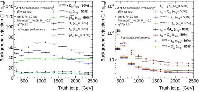
Different combinations of 2 variables are tested and their performance is compared at signal efficiencies of 50% and 80% with a parametrization yielding flat signal efficiencies as a function the jet p

T

. The resulting background rejection versus p

T

distributions are shown in Figure 3 for the best performing combinations found.

The two-variable combinations that provided the best overall performance for W-boson and top-quark tagging were chosen:

• combined jet mass and D

for W -boson tagging and

•

√ d

and τ

for top-quark tagging.

For the chosen taggers the working points are re-defined as a function of the reconstructed jet p

and they are parametrized so that they yield flat signal efficiencies versus p

. In addition, only one efficiency working point parametrized in p

will be presented in the following: 50% for W -boson tagging and 80%

for top-quark tagging, as those are commonly used in ATLAS analyses.

[GeV]

Truth jet pT

500 1000 1500 2000 2500

)bkg∈Background rejection (1 /

0 20 40 60 80 100 120

140 ATLAS Simulation Preliminary = 13 TeV

s

R=1.0 jets anti-kt

=0.2)

=0.05, Rsub

Trimmed(fcut

|<2.0

truth

η

|

tagger performance W

= 50%)

∈sig 2 (

comb + D m

)

= 50%

∈sig 21 ( τ

comb + m

)

= 50%

∈sig 12 ( d

comb + m

= 80%)

∈sig 2 (

comb + D m

= 80%)

∈sig 21 ( τ

comb + m

= 80%)

∈sig 12 ( d

comb + m

[GeV]

Truth jet pT

500 1000 1500 2000 2500

)bkg∈Background rejection (1 / 10

102

103 ATLAS Simulation Preliminary = 13 TeV

s

R=1.0 jets anti-kt

=0.2)

=0.05, Rsub

Trimmed(fcut

|<2.0

truth

η

|

Top tagger performance

= 50%)

∈sig 23 ( d

32 + τ

= 50%)

∈sig W (

32 + Q τ

= 50%)

∈sig 32 ( τ

comb + m

= 50%)

∈sig W (

comb + Q m

= 80%)

∈sig 23 ( d

32 + τ

)

= 80%

∈sig W (

32 + Q τ

)

= 80%

∈sig 32 ( τ

comb + m

)

= 80%

∈sig W (

comb + Q m

Figure 3: W-boson (left) and top-quark tagging (right) background rejection distributions as a function of p_Tfor the best performing two-variable combinations at 50% and 80% signal efficiency.

5.2 Deep neural network and boosted decision tree based taggers

Some of the observables described in Section 4 contain complementary information. It has been shown that

the combination of these observables to create a multivariate W -boson or top-quark classifier provides

higher discrimination, albeit to differing degrees [56–58]. In this work boosted decision tree (BDT)

and deep neural network (DNN) algorithms are applied to explore such techniques following a similar

Tagging Type Observable Set

W-boson tagging

m^comb,p_T e₃,C₂,D₂ τ₁,τ₂,τ₂₁

R^FW

2 , P,a₃,A Z_cut,

√ d₁₂ KtDR

Top-Quark Tagging

m^comb,p_T e₃,C₂,D₂ τ₁,τ₂,τ₃,τ₃₂,τ₂₁

√ d₁₂,

√ d₂₃,Q_W

Table 3: Summary of variables used in the DNN and BDT taggers studies forW-boson and top-quark tagging. Here e₃is defined ase₃=ECF₃/ECF³

1.

procedure as Ref. [58] and the ability of these algorithms to discriminate W -boson and top-quark jets from the gluon and light-quark jet background are studied in parallel. Study of these two algorithms in parallel is motivated to explore if one of the architectures is better suited to exploit input correlations among high-level variables, and to study the performance of both algorithms when applied to data.

The BDT and DNN used here are similar to the ones described in detail in Ref. [58]. The description of the training criteria, of the training and testing sets, and of the relevant event weights is not repeated here. A similar hyperparameter scan was performed yielding similar results. While the procedure has only changed minimally in comparison to the one in Ref. [58], the choice of input observables are slightly adapted and they are shown in Table 3. As the jet mass is now used as an input, the BDT and DNN taggers in this work do not use an additional mass cut except the very low mass threshold that is part of the training criteria

. Although the BDT and DNN optimization studies are carried out using only the jets that satisfy the training criteria, the discrimination power obtained by m

> 40 GeV is included as part of the BDT and DNN taggers in Section 5.3 in order to compare taggers using jets with similar kinematics as inputs

. Additionally, the optimization studies are carried out in a wide p

T

bin and the relative performance gain is evaluated with flat p

T

spectra. However, the comparison of taggers in Section 5.3 is made with p

T

distributions for signal jets weighted to match that of the dijet background samples.

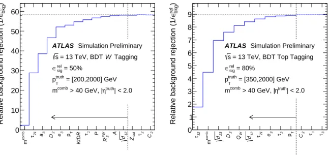
To find the optimal set of BDT input variables, single input variables that give the largest increase in relative performance are sequentially added to the network. This procedure is initiated with the input variables listed in Table 3. The relative performance is evaluated using jets from the testing sample which pass the training criteria and with the training weights described in Ref. [58] in the kinematic range 200 < p

T

< 2000 GeV. During the input and hyperparameter optimization of the multivariate techniques, the jets which do not pass the jet mass ( m

> 40 GeV) and number of constituents ( N

> 2) training criteria are not included in the relative signal efficiency or background rejection evaluation.

At each step, the variable which gives the greatest increase in relative background rejection at a fixed relative signal efficiency of 50% ( W -boson tagging) and 80% (top-quark tagging), when added to the existing set of variables, is retained. The minimum set of variables which reaches the highest relative

5To ensure that all used jet substructure features are well defined for the training jets, two additional selection criteria are applied on the jet mass (m^comb >40 GeV) and number of constituents (N^const>2). The jets which fail the training criteria are not used in the training.

6Jets that fail the mass criteria are tagged as background jets. Jets that pass the mass requirement but fail the number of constituents requirement are tagged as signal jets. The fraction of jets found to be categorized in this way is less than 1%.

background rejection within statistical uncertainties are selected. The minimal number of variables is 12 for W -boson tagging and 10 for top-quark tagging. The relative background rejections achieved are shown in Figure 4.

combm 21τ 3a 2D 3e Tp KtDR 1τ P FW 2R A 12d cutZ 2τ 2C

)bkgrel∈Relative background rejection (1/

0 10 20 30 40 50 60

ATLAS Simulation Preliminary Tagging W

= 13 TeV, BDT s

= 50%

rel

∈ sig

= [200,2000] GeV

truth

pT

| < 2.0

truth

η > 40 GeV, | mcomb

32τ combm 23d 2D WQ 12d 21τ 3e 2τ Tp 2C 1τ 3τ

)bkgrel∈Relative background rejection (1/

0 1 2 3 4 5 6 7 8 9

ATLAS Simulation Preliminary = 13 TeV, BDT Top Tagging s

= 80%

rel

∈ sig

= [350,2000] GeV

truth

pT

| < 2.0

truth

η > 40 GeV, | mcomb

Figure 4: BDT relative background rejection (blue) for different sets of variables with successively adding more variables at the 50%(W-boson tagging) and 80% (top-quark tagging) relative signal efficiency working point forW- boson (left) and top-quark tagging (right). Only jets which pass the training criteria are considered while calculating the relative signal efficiency and relative background rejection. The performance is evaluated with flatp^truth

T spectra.

Uncertainties are not presented.

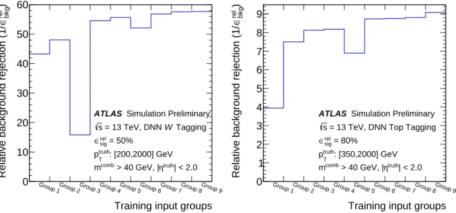
Similar to the BDT training, the DNN is trained on different sets of input variables in order to find the

optimal set of input variables with the training weights described in Ref. [58]. The relative performance

is evaluated using the jets in the testing set that pass the training criteria. Unlike the BDT, sets of

input variables are not defined by successively adding variables but are defined by grouping the inputs

variables related to the corresponding signal. The grouping is chosen by selecting variables based on their

dependence on the momentum scale of the jet’s substructure objects, on what features of the substructure

they describe and on their dependence on other substructure variables. A summary of all the variables

tested for the DNN is shown in Tables 4 and 5. The relative background rejections achieved inclusively

in jet p

are presented in Figure 5. As observed in Ref. [58], the performance of the DNN tagger depends

both on the number of variables and the information content in the group. The chosen groups of inputs

for W -boson tagging and top-quark tagging are listed in Table 6. Within the statistical uncertainties the

number of variables necessary for maximum rejection at the relative fixed signal efficiency (50% for

W -boson, 80% for top-quark) is found to be 12 variables for W -boson tagging (Group 8 in Table 4) and

13 variables for top-quark tagging (Group 9 in Table 5).

Group 1 τ

, τ

, e

, m

, p

Group 2 τ

, τ

, e

, m

, p

,

√ d

, KtDR Group 3 τ

, C

, D

, R

2

, P , a

, A , Z

Group 4 τ

, C

, D

, R

2

, P , a

, A , Z

, m

Group 5 τ

, C

, D

, R

2

, P , a

, A , Z

, m

, p

Group 6 τ

, τ

, e

, m

, p

, R

2

,

√ d

, KtDR, a

, A Group 7 τ

, C

, D

, R

2

, P , a

, A , Z

, m

,

√ d

, KtDR Group 8 τ

, C

, D

, R

2

, P , a

, A , Z

, m

, p

,

√ d

, KtDR Group 9 τ

, τ

, τ

,

√ d

, C

, D

, e

, m

, p

, R

2

, P , a

, A , Z

, KtDR

Group 1 C

, D

, τ

, τ

, Group 2 C

, D

, τ

, τ

, m

Group 3 C

, D

, τ

, τ

, m

, p

Group 4 τ

, τ

, τ

, e

, m

, p

Group 5 C

, D

, τ

, τ

,

√ d

,

√ d

, Q

Group 6 C

, D

, τ

, τ

,

√ d

,

√ d

, Q

, m

Group 7 τ

, τ

, τ

, e

, m

, p

,

√ d

,

√ d

, Q

Group 8 C

, D

, τ

, τ

,

√ d

,

√ d

, Q

, m

, p

Group 9 τ

, τ

, τ

, τ

, τ

,

√ d

,

√ d

, Q

, C

, D

, e

, m

, p

5.3 Summary of tagger performance studies in simulation

The discrimination power of the taggers studied is compared in this section in two ways. First, for various taggers the background rejection versus the signal efficency is shown in receiver operating characteristic (ROC) curves. In addition, the background rejection versus the p

T

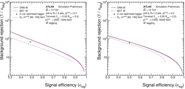
is presented for fixed signal efficiencies. For W -boson tagging, four taggers are compared:

• BDT W -boson and DNN W -boson taggers are both composed of a requirement on the relevant discriminant described in Section 5.2, optimized for W -boson tagging, and a fixed m

requirement of m

> 40 GeV. The requirement on the BDT or DNN discriminant is varied to obtain the desired signal efficiency.

• Simple m

+ D

is composed of a pre-defined fixed mass requirement of 60 < m

< 120 GeV and a varying D

requirement chosen to obtain the desired signal efficiency. This simple tagger is included for comparison purposes.

• The two-variable optimized 50% W -boson tagger is composed of a varying m

and D

require- ment as described in Section 5.1. As this tagger is designed and optimized for the specific fixed signal efficiency working points, it is represented by a point in Figure 6 that gives the desired signal efficiency chosen for comparison.

For top-quark tagging, six taggers are compared:

• BDT top-quark and DNN top-quark taggers are both composed of a requirement on the relevant

discriminant described in Section 5.2, optimized for top-quark tagging, and a fixed m

require-

Training input groups

Group 1Group 2Group 3Group 4Group 5Group 6Group 7Group 8Group 9

)

rel bkg

∈Relative background rejection (1/

0 10 20 30 40 50 60

ATLAS Simulation Preliminary Tagging W = 13 TeV, DNN s

= 50%

rel

∈ sig

: [200,2000] GeV

truth

pT

| < 2.0

truth

η > 40 GeV, | mcomb

Training input groups

Group 1Group 2Group 3Group 4Group 5Group 6Group 7Group 8Group 9

)

rel bkg

∈Relative background rejection (1/

0 1 2 3 4 5 6 7 8 9

ATLAS Simulation Preliminary = 13 TeV, DNN Top Tagging s

= 80%

rel

∈ sig

: [350,2000] GeV

truth

pT

| < 2.0

truth

η > 40 GeV, | mcomb

Figure 5: Distributions showing the training with different set of variables and relative improvement in performance for the DNNW-boson and top-quark taggers at the 50% and 80% relative signal efficiency working point, respectively.

Only jets which pass the training criteria are considered while calculating the relative signal efficiency and relative background rejection. The performance is evaluated with flatp^truth

T spectra. Uncertainties are not presented.

W -Boson Tagging Top-Quark Tagging

Observable BDT DNN BDT DNN

m

◦ ◦ ◦ ◦

p

◦ ◦ ◦ ◦

e

◦ ◦ ◦

C

◦ ◦

D

◦ ◦ ◦ ◦

τ

◦ ◦

τ

◦ ◦

τ

◦

τ

◦ ◦ ◦ ◦

τ

◦ ◦

R

2

◦ ◦

P ◦ ◦

a

◦ ◦

A ◦ ◦

Z

◦

√ d

◦ ◦ ◦ ◦

√ d

◦ ◦

Kt DR ◦ ◦

Q

◦ ◦

Table 6: Summary of the set of observables that are chosen with respect to Figures4and5.

ment of m

> 40 GeV. The requirement on the BDT or DNN discriminant is varied to obtain the desired signal efficiency.

• The shower deconstruction tagger is composed of a requirement on the log χ variable described in Section 4.3.2 and a fixed m

requirement of m

> 60 GeV. Similar to the BDT and DNN taggers, the requirement on log χ is varied to obtain the desired signal efficiency.

• The HEPTopTagger selection consists of identifing a top-quark candidate followed by a mass requirement of 140 < m

< 210 GeV on this candidate. This tagger is represented by a point in Figure 7 as it provides a working point in each p

bin.

• A tagger using the m

and τ

variables requires a fixed m

> 60 GeV and a varying maximum τ

cut to obtain the desired signal efficiency. This simple tagger is included for comparison purposes.

• The two-variable optimized 80% top-quark tagger is composed of a varying

√ d

and τ

require- ment as described in Section 5.1. As this tagger is optimized for the specific fixed signal efficiency working points, it is represented by a point in Figure 7 that gives the desired signal efficiency chosen for comparison.

The performance of the taggers is evaluated in two wide jet p

T

bins in terms of ROC curves, as shown in Figures 6 and 7 for the W -boson and top-quark taggers, respectively. Furthermore, the background rejection at the fixed 50% and 80% signal efficiency working point

as a function of p

are presented for W -boson and top-quark tagging, respectively, in Figure 8.

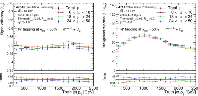
The dependence of the taggers on the pile-up conditions is illustrated in Figures 9 and 10 using the two- variable W -boson and top-quark taggers optimized for the full dataset (independent of the average number of interactions in the event) as examples and showing the signal efficiency and background rejection obtained for different average number of interactions µ . While the top-quark tagger shows hardly any dependence ( < 1%) on the pile-up conditions, there is some dependence for the W -boson tagger due to the use of the D

variable that is more sensitive to pile-up. At the 50% working point, the variation in the W -boson tagger efficiency and background rejection in different µ ranges is observed to be up to 5% and 6%, respectively.

For W -boson tagging the best performing taggers are the DNN and BDT taggers over the whole range in p

studied. They perform very similarly and outperform the two-variable tagger, especially at low p

. The optimization of the two-variable taggers yields a better performance than the cut and scan combination of the same variables.

For top-quark tagging the DNN and BDT taggers also yield the best performance over the full p

range.

They show very similar performance overall, with the BDT being a bit better at low signal efficiencies and p

. Shower deconstruction algorithm yields the best non multivariate result, with the much simpler HEPTopTagger (in its original version) being close in performance. The HEPTopTagger is the only tagger able to tag top quarks down to a p

of 200 GeV.

In the next sections, the taggers that are compared in this section are applied to data and compared to MC samples. For this purpose working points are defined for the BDT, DNN, shower deconstruction taggers and they are parametrized so that they yield flat signal efficiencies versus reconstructed jet p

like the two-variable taggers.

7HEPTopTagger is not included in this comparison as it provides a single working point in eachp_Tbin.

sig) Signal efficiency (∈

0.3 0.4 0.5 0.6 0.7 0.8 0.9 1

)bkg∈Background rejection (1 /

1 10 102

103

104

ATLAS Simulation Preliminary = 13 TeV

s

| < 2.0

truth

R=1.0 jets, |η anti-kt

= 0.2) = 0.05 Rsub

Trimmed (fcut

= [500, 1000] GeV

truth

pT

tagging W DNN W

BDT W

2−var optimised tagger [60, 100] GeV , mcomb

D2

sig) Signal efficiency (∈

0.3 0.4 0.5 0.6 0.7 0.8 0.9 1

)bkg∈Background rejection (1 /

1 10 102

103

104

ATLAS Simulation Preliminary = 13 TeV

s

| < 2.0

truth

R=1.0 jets, |η anti-kt

= 0.2) = 0.05 Rsub

Trimmed (fcut

= [1500, 2000] GeV

truth

pT

tagging W DNN W

BDT W

2−var optimised tagger [60, 100] GeV , mcomb

D2

Figure 6: The performance comparison of theW-boson taggers in a low-p^truth

T (left) and high-p^truth

T (right) bin. The performance is evaluated with thep^truth

T distribution of the signal jets weighted to match that of the dijet background samples.

sig) Signal efficiency (∈

0.3 0.4 0.5 0.6 0.7 0.8 0.9 1

)bkg∈Background rejection (1 /

1 10 102

103

104

ATLAS Simulation Preliminary = 13 TeV

s

| < 2.0

truth

R=1.0 jets, |η anti-kt

= 0.2) = 0.05 Rsub

Trimmed (fcut

= [500, 1000] GeV

truth

pT

Top tagging DNN top

BDT top

Shower Deconstruction 2-var optimised tagger HEPTopTagger v1

> 60 GeV , mcomb

τ32

sig) Signal efficiency (∈

0.3 0.4 0.5 0.6 0.7 0.8 0.9 1

)bkg∈Background rejection (1 /

1 10 102

103

104

ATLAS Simulation Preliminary = 13 TeV

s

| < 2.0

truth

R=1.0 jets, |η anti-kt

= 0.2) = 0.05 Rsub

Trimmed (fcut

= [1500, 2000] GeV

truth

pT

Top tagging DNN top

BDT top

Shower Deconstruction 2-var optimised tagger HEPTopTagger v1

> 60 GeV , mcomb

τ32

Figure 7: The performance comparison of the top-quark taggers in a low-p^truth

T (left) and high-p^truth

T (right) bin. The performance is evaluated with thep^truth

T distribution of the signal jets weighted to match that of the dijet background samples.