Analyzing the Optimization Potential of Steam Production in Waste-to-Energy Plants: Examples by Evaluating Data from Three Different Plants

(1)

227 Analyzing the Optimization Potential of Steam Production in Waste-to-Energy Plants

Waste Incineration

Analyzing the Optimization Potential of Steam Production in Waste-to-Energy Plants: Examples by Evaluating Data

from Three Different Plants

^*

Therese Schwarzböck, Helmut Rechberger and Johann Fellner

1. Material and methods ...229

1.1. Determining the waste feed composition by applying the Balance Method ...229

1.2. Analysing the variability of the steam production ...229

2. Results ...230

2.1. Variability of steam production ...230

2.2. Relation between variable steam production and waste characteristics .232 2.3. Effect of variable waste composition on steam production ...236

3. Conclusions ...239

4. Literature ...239 In many affluent countries, energy recovery from waste has become an important part of their waste management, resource recovery and energy supply strategies. It is regarded as a viable treatment option to save land for landfill facilities, to significantly reduce waste volumes, and to completely disinfect waste. While these aspects have been the main arguments in the past, developments in recent years depict Waste-to-Energy (WtE) as important tool for material recycling and resource conservation [2, 7, 15].

Thus, driven by the climate debate, the promotion of renewable energies and the demand for high energy efficiencies, the efficient recovery of energy from waste is becoming increasingly important. On the one hand, the energy gained represents an important source of income for WtE plant operators, on the other hand, efficient recovery of energy indirectly reduces the greenhouse gas emissions from WtE plants (through the higher substitution of fossil fuels). However, compared to conventional thermal power plants (coal, gas, fuel oil), energy efficiencies of WtE plants are significantly lower [2, 3, 14]. This is primarily due to three factors:

a) steam parameters of WtE boilers are significantly lower than those of conventional thermal power plants, because of the highly corrosive properties of waste flue gas (mainly due to high Cl content),

b) a higher air surplus is required as a buffer due to fluctuations (and heterogeneity) of the waste,

c) energy input from waste is not constant as for conventional fossil fuel power plants, but subject to considerable temporal fluctuations, depending on its composition (variable calorific value).

* peer reviewed paper

(2)

Therese Schwarzböck, Helmut Rechberger, Johann Fellner

228

Waste Incineration

Factor a) is partially compensated by extracting heat only (provided that there is demand for heat) or by reheating the steam between high pressure and low pressure stage of the turbine. Furthermore, in certain WtE plants higher steam parameters are attempted to be achieved by increased corrosion protection (cladding of the boiler flues), which lead to a higher total electrical efficiency (e.g. WtE plant in Amsterdam, planned WtE plant in Shenzhen) [8, 9].

Factors b) and c) both arise from variations in waste composition, which are usually unavoidable. The composition of the delivered waste is influenced by the settlement structure, social disparities in the catchment area of the WtE plant, seasonal factors as well as the type of waste (household waste, commercial waste, industrial waste, etc.) [5, 6]. By mixing the delivered waste in the bunker of the WtE plant, the operator tries to compensate for the varying composition. This attempt to homogenize the waste (e.g.

in terms of calorific value, water content or ash content), is beneficial for the energy efficiency but also reduces emissions of air pollutants (such as CO, NO_x, or dioxins). In particular, emission peaks, which are primarily caused by unstable operation of the plant (fluctuating firing capacity) and insufficient burnout, are thereby avoided [1, 3, 13-15].

However, so far, it cannot be assessed if waste mixing in the bunker is conducted suffi- ciently, as there is a lack of information on the short-term variability of the waste feed composition. Thus, the changing waste feed composition cannot be considered in the combustion control system [16]. First investigations by the authors at one WtE plant showed that the so-called Balance Method [4] can potentially be utilized to deliver appropriate data on the short-term variation in waste composition (e.g. hourly data on the share of biomass in the waste). Furthermore, it was shown that short-term changes (hourly) in waste composition are much more pronounced compared to variations in daily means or monthly means [10, 12].

The paper presents the first detailed analysis of the effect of changing waste feed composition in WtE plants on different operating data, such as steam production, auxiliary fuel consumption, waste throughput or excess air. The analysis is done by empirical statistical evaluations of real WtE plant operating data. Data from three WtE plants are evaluated at a high temporal resolution (hourly values) over a period of one year.

In particular, the following general questions are addressed:

• Which factors lead to a variability of the steam production and which parameters could be used as indication for an unstable steam production?

• Is there a connection between variability in steam production and the variability in waste feed composition?

• Which losses of steam production can be expected to be avoided when mixing of the bunker waste is improved (thereby reducing the temporal variability of the waste composition)?

A further objective of the paper is to evaluate the suitability of the Balance Method for the purpose of detecting short-term fluctuations of the waste composition (e.g.

biomass share) and thus, providing a potential tool to avoid insufficiently mixed waste on the grate.

(3)

Waste Incineration

1. Material and methods

The conducted analysis is based on the evaluation of real operating data from three different WtE plants over a period of one year. All three WtE plants are equipped with a grate firing system and have a capacity between 100,000 and 300,000 tons of waste per year. Hourly values during regular operation of the plant are used for the empirical statistical analyses. Shut-down and start-up periods are disregarded because they are considered as unavoidable due to annually required plant revisions. The analyses are conducted with data which are measured directly at the plants as well as with data which have been calculated by means of the Balance Method.

1.1. Determining the waste feed composition by applying the Balance Method

The Balance Method is used to generate data on the waste feed characteristics in the WtE plants. The method is based on different material and energy balances, which use plant operating data and information upon the elemental composition of biogenic and fossil materials. This allows the content of biogenic (biomass) and of fossil materials (plastics) to be determined [4]. The calculations based on the Balance Method are integrated into the Software BIOMA, which can be applied to WtE plant operating data (https://iwr.

tuwien.ac.at/ressourcen/downloads/bioma/) and which is used in the presented study.

Waste composition data is provided by BIOMA based on the following mass shares:

Biomass share, fossil share (plastics), share of water, share of inert materials and metals.

Different to previous (common) evaluations by means of the Balance Method (e.g.

[11]), the output data are generated on an hourly basis instead of monthly or annual averages. This possibility to generate high temporal resolution data by means of the Balance Method (restricted only by the temporal resolution of the input operating data) is considered as a chance to provide valuable information to the plant operators on short-term change of waste characteristics. The following output parameter of the Balance Method are used in the presented investigations: water content of waste feed (m_W), share of biomass in waste feed (m_B), and lower heating value of waste feed (LHV).

1.2. Analysing the variability of the steam production

The variability of the steam production is compared with different plant operation characteristics (steam production, waste throughput, O₂-content in the flue gas, utilization of auxiliary fuels) and with different waste characteristics (m_W, m_B, LHV) and their respective variability. The comparisons are made in order to ascertain if an unstable steam production is generally connected with lower efficiency of the plant operation (higher excess air, lower steam production) and if the assumption that a varying steam production is caused by the heterogeneity of the waste composition, is valid.

The variability of the different parameters is defined as standard deviation (SD) over a period of six consecutive hours. All data during start-up and shut-down times are excluded from the conducted statistical analyses. Empirical cumulative distribution

(4)

230

Waste Incineration

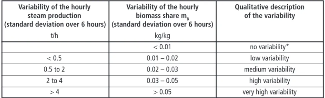
functions are applied to hourly values and to the 6-hours SD. The variability of the steam production and of the biomass share m_B is divided into different categories as listed in Table 1. Figure 1 shows an example of varying steam production over a period of around three days.

Table 1: Categories of variability for the parameter steam production and biomass share (m_B) Variability of the hourly Variability of the hourly Qualitative description steam production biomass share m_B of the variability (standard deviation over 6 hours) (standard deviation over 6 hours)

t/h kg/kg

< 0.01 no variability*

< 0.5 0.01 – 0.02 low variability

0.5 to 2 0.02 – 0.03 medium variability

2 to 4 0.03 – 0.05 high variability

> 4 > 0.05 very high variability

* times declared with no variability in mB are used to calculate the reference steam production

Figure 1: Example of the hourly steam production (given relatively to the target hourly steam production) and hourly usage of auxiliary fuel over a period of 80 hours for a Waste-to- Energy plant

2. Results

2.1. Variability of steam production

Figure 2 to Figure 5 show the relative cumulative frequency of different plant operation parameter compared with the variability of the steam production. It can be seen that a higher variability of the steam production (given as standard deviation over a period of six consecutive operating hours) is connected with a lower steam production by trend for all three plants. When there is a low variability of the steam production

0 0.2 0.4 0.6 0.8 1.0

Relative steam production t/t

Relative steam production

0 1 2 3 4 5 Auxiliary fuel consumption t/h

Auxiliary fuel consumption

period with medium variability of

steam production period with very high variability of steam production

00:0004:00 08:00 12:00 16:00 20:00 00:00 04:00 08:00 12:00 16:00 20:00 00:00 04:0008:0012:00 16:00 20:00 00:0004:0008:00

(5)

Waste Incineration

(SD below 0.5 t/h, blue line in Figure 2), then at least 90 % of the target steam production is reached during more than 90 % of the time. At high variability (SD above 4 t/h, red line in Figure 2), 90 % of the target steam production is only reached during 60 % (WtE A, WtE B) to 80 % (WtE C) of the time.

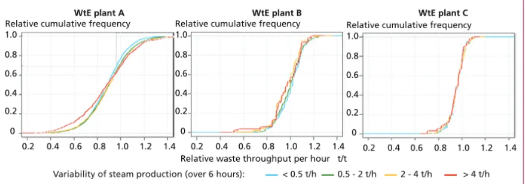
When comparing the variability in the steam production to the waste throughput (Fig- ure 3), there is no clear trend between waste throughput and unstable steam production.

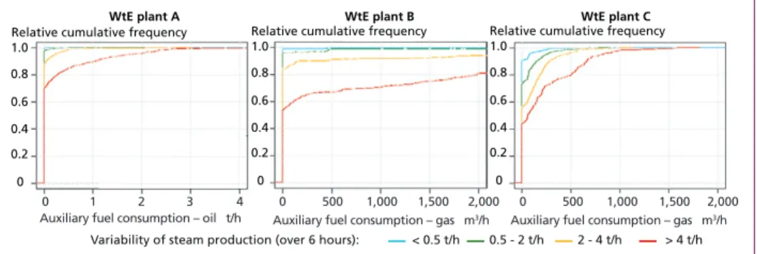
From Figure 4 it can be expected that a higher instability of the steam production is connected with a higher excess air (as indicated by an increasing oxygen concentration in the flue gas) for all plants. This indicates that a lower boiler efficiency (due to higher flue gas volume) is reached when the steam production is not stable. Finally, also the demand for auxiliary fuels (heating oil, natural gas) is elevated when the variability of the steam production is high (Figure 5).

For all regarded three plants, Figure 2 to Figure 5 show that there is a general interrelation between different plant operating parameters and an unstable steam production.

Hence, it can be assumed that the variability of the steam production gives an indication of the degree of stability or instability of the WtE plant operation.

Figure 2: Relative cumulative frequencies of hourly steam production (referred to the target hourly steam production) for different variability categories of steam production (given as standard deviation over a period of six hours); hourly operating data over a period of one year are considered

0.4 0.5 0.6 0.7 0.8 0.9 1.0 1.1 Relative cumulative frequency

0 0.2 0.4 0.6 0.8 1.0

WtE plant C

0.4 0.5 0.6 0.7 0.8 0.9 1.0 1.1 Relative cumulative frequency

0 0.2 0.4 0.6 0.8 1.0

Relative cumulative frequency

0 0.2 0.4 0.6 0.8 1.0

WtE plant A WtE plant B

Relative steam production per hour t/t 0.4 0.5 0.6 0.7 0.8 0.9 1.0 1.1

Variability of steam production (over 6 hours): < 0.5 t/h 0.5 - 2 t/h 2 - 4 t/h > 4 t/h

0.2 0.2

0 0.4 0.4

0.6 0.6

0.8 0.8

1.0 1.0

1.4 0.2 0.4 0.6 0.8 1.0 1.2 1.4 1.2

Relative waste throughput per hour t/t 0.2 0.4 0.6 0.8 1.0 1.2 1.4

0.2 0 0.4 0.6 0.8 1.0

WtE plant A WtE plant B WtE plant C

Figure 3: Relative cumulative frequencies of hourly waste throughput (referred to the average hourly waste throughput) for different variability categories of steam production (given as standard deviation over a period of six hours); considering data over a period of one year

(6)

232

Waste Incineration

WtE plant C

0.2 0 0.4 0.6 0.8 1.0

WtE plant A WtE plant B

0.2 0 0.4 0.6 0.8 1.0

6 8 10 12 14

O₂-concentration in the flue gas Vol-%

6 8 10 12 14 6 8 10 12 14

Figure 4: Relative cumulative frequencies of oxygen concentration in the flue gas for different variability categories of steam production (given as standard deviation over a period of six hours); considering data over a period of one year

Figure 5: Relative cumulative frequencies of the demand for auxiliary fuels (heating oil, natural gas) for different variability categories of steam production (given as standard deviation over a period of six hours); considering data over a period of one year

2.2. Relation between variable steam production and waste characteristics

Figure 6 to Figure 8 compare different waste characteristics (water content m_W, biomass share m_B, lower heating value LHV) to the variability of the steam production for the different plants. The presented waste characteristics do all represent parameters, which are determined by the Balance Method (output parameter of the software BIOMA).

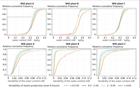
The results show that for WtE plant B, a high variability of the steam production (SD > 4 t/h) is connected with a higher m_W and thus, a lower m_B (on a dry basis) and a lower LHV of the waste feed (upper middle graph in Figure 6 to Figure 8). This indicates that in this plant, the water content of the waste (which is in average above the ones in WtE plant A and C) affects the stability of the steam production. For WtE plant A and WtE plant C, this interrelation is less apparent (upper left and upper right graph in Figure 6).

However, the relation between a variable steam production and LHV is observable for all three plants, whereby least distinct for WtE plant C (Figure 8 upper graphs).

Comparing the graphs for WtE plant C for the parameter m_W, m_B, and LHV in Figure 6 to Figure 8 show that m_B is rather diverse in this plant in the course of one year (flat curve for upper right graph in Figure 7). Still, the curves for m_W and LHV for WtE plant C are in a narrow range (steep curves in upper right graphs of Figure 6 and Figure 8).

0.2 0 0.4 0.6 0.8 1.0

Relative cumulative frequency WtE plant A

0.2 0 0.4 0.6 0.8 1.0

Relative cumulative frequency WtE plant B

0.2 0 0.4 0.6 0.8 1.0

Relative cumulative frequencyWtE plant C

Auxiliary fuel consumption – oil t/h

0 1 2 3 4

Auxiliary fuel consumption – gas m³/h

0 500 1,000 1,500 2,000

Auxiliary fuel consumption – gas m³/h 1,500 2,000

0 500 1,000

(7)

STANDARDKESSEL BAUMGARTE - Power plants, plant operation and services for generating electricity, steam and heat from residues, primary fuels, waste heat and biomass.

Energy costs are continually rising. Making it all the more important for companies and municipalities to explore cheaper fuel alternatives for their energy supply.

We are experts in them: household and commercial waste, industrial residues and refuse derived fuels. And for many years now, we have been proving how they can be used in thermal recycling processes to produce useable energy for generating electricity, process steam and district heat.

For more information and references, visit:

www.standardkessel-baumgarte.com

TONS OF ENERGY!

ENERGY GENERATION FROM RESIDUES:

EFFICIENT & ECO-FRIENDLY.

(8)

www.emea.mhps.com Integrated Power Generation Solutions

Mitsubishi Hitachi Power Systems Europe supplies up-to-date, efficient products. We construct most modern power plants and Waste-to-Energy plants. And we deliver reliable and cost- effective service solutions. Our green technologies – in energy storage and biomass, for instance – are examples for our innovation capabilities. Intelligent power generation solutions require know-how and experience. Mitsubishi Hitachi Power Systems has them both – making us a globally successful energy plant constructor and service provider.

Joint Forces

(9)

Waste Incineration

Figure 6: Relative cumulative frequencies of water content (m_W) of the waste feed (top row), and relative cumulative frequencies of variability of m_W (given as SD over a period of six hours) (bottom row) for different variability categories of steam production (given as SD over a period of six hours); hourly operating data over a period of one year are considered for each graph

Figure 7: Relative cumulative frequencies of biomass share (m_B) in the waste feed (top row), and relative cumulative frequencies of variability of m_B (given as SD over a period of six hours) (bottom row) for different variability categories of steam production (given as SD over a period of six hours); hourly operating data over a period of one year are considered for each graph

0.2 0

0 0.1 0.2 0.3 0.4 0.5

0 0.02 0.04 0.06 0.08 0.10 0.12 0.4

0.6 0.8 1.0

Biomass share m_B kg/kg 0 Biomass share m0.1 0.2 0.3_B kg/kg0.4 0.5 0 0.1Biomass share m0.2 0.3_B kg/kg0.4 0.5 0.2

0 0.4 0.6 0.8 1.0

0.2 0 0.4 0.6 0.8 1.0

Variability of biomass share m_B 0 0.02 0.04 0.06 0.08 0.10 0.12

Variability of biomass share m_B 0 0.02 0.04 0.06 0.08 0.10 0.12 Variability of biomass share m_B

Variability of steam production (over 6 hours): < 0.5 t/h 0.5 - 2 t/h 2 - 4 t/h > 4 t/h 0.2

0

0 0.1 0.2 0.3 0.4 0.5

0 0.02 0.04 0.06 0.08 0.10 0.12 0.4

0.6 0.8 1.0

water content mW kg/kg 0 0.1 0.2 0.3 0.4 0.5

water content mW kg/kg 0.2

0 0.4 0.6 0.8 1.0

0.2 0 0.4 0.6 0.8 1.0

Variability of the water content mW 0 0.02 0.04 0.06 0.08 0.10 0.12

Variability of the water content mW 0 0.02 0.04 0.06 0.08 0.10 0.12 Variability of the water content mW Variability of steam production (over 6 hours): < 0.5 t/h 0.5 - 2 t/h 2 - 4 t/h > 4 t/h

(10)

236

Waste Incineration

These different frequency curve appearances for WtE plant C suggest that the varying waste feed composition in terms of biomass content can generally be better compensated than in the other two plants. A better waste mixing (or easier mixable waste) can be expected for WtE plant C. However, high short-term variabilities (here: 6 hours) for m_W, m_B and LHV of the waste, appears to be linked with a high variability of the steam production in all three plants (bottom graphs in Figure 6 to Figure 8). Thus, a (short-term) change in the waste composition (e.g. from 25 to 30 weight-% of biomass in the waste within a few hours) leads to an unstable plant operation (lower steam production, lower efficiency).

2.3. Effect of variable waste composition on steam production

Based on the analyses in the previous chapter, the variability of both parameters m_B (biomass share) and m_W (water content) appear to be appropriate indicators for a changing waste composition (and thus the heterogeneity of the waste feed). In this chapter, the waste heterogeneity based on the parameter m_B is directly compared to the steam production. Expected losses of the steam production are estimated when m_B is varying at certain levels. Thereto, five different categories for the variability of m_B are defined (see Table 1) and the respective data on the hourly steam production are assigned. The first category (m_B variability < 1 weight-%) is used to define the reference Figure 8: Relative cumulative frequencies of lower heating value (LHV) of the waste feed (top row), and relative cumulative frequencies of variability of LHV (given as SD over a period of six hours) (bottom row) for different variability categories of steam production (given as SD over a period of six hours); hourly operating data over a period of one year are considered for each graph

0.2 0

4,000 6,000 8,000 10,000 12,000 14,000 0.4

0.6 0.8 1.0

Lower heating value LHV kJ/kg Lower heating value LHV kJ/kg Lower heating value LHV kJ/kg 0.2

0 0.4 0.6 0.8 1.0

0.2 0 0.4 0.6 0.8 1.0

Variability of lower heating value LHV Variability of lower heating value LHV Variability of lower heating value LHV 4,000 6,000 8,000 10,000 12,000 14,000 4,000 6,000 8,000 10,000 12,000 14,000

0 1,000 2,000 3,000 4,000 0 1,000 2,000 3,000 4,000 0 1,000 2,000 3,000 4,000

(11)

Waste Incineration

steam production (mean value). Based on this reference value, the differences per hour to the actual steam production are calculated and presented as relative difference in Figure 9 to Figure 11 depending on the variability of m_B.

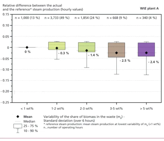
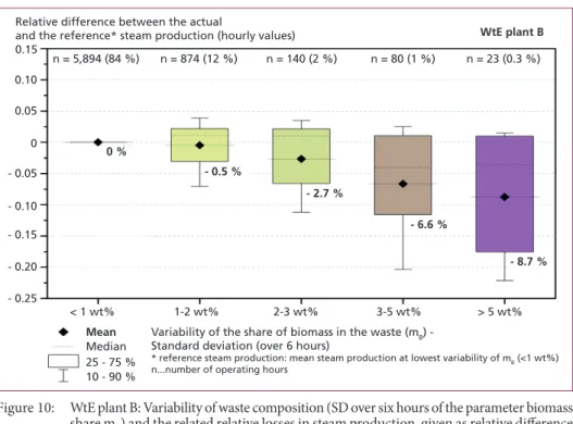
The results show that there are losses in steam production with increasing variability of the biomass share. The highest losses (-8.7 %) are expected for WtE plant B when there is a variability of m_B of above 5 weight-%. However, this high variability is only occurring during a very limited number of time (0.3 % of the regarded hours). The highest total losses (or optimization potential by better mixing of the waste feed) of steam production during times of high variable waste composition are expected for WtE plant A (Figure 9). In average, a reduced steam production of 2.5 % is found when m_B is varying in average by more than 3 weight-% (over six hours). This variation occurs during 13 % (sum of 9 % and 4 % as given in Figure 9) of the regular operating hours.

For WtE plant C, the steam production losses due to the variability of the waste feed can be estimated to be below 0.5 % (Figure 11). A low heterogeneity of the waste feed (and thus a good mixing of the waste in the bunker) of WtE plant C can be expected.

Figure 9: WtE plant A: Variability of waste composition (SD over six hours of the parameter biomass share m_B) and the related relative losses in steam production, given as relative difference between the actual hourly steam production and the reference steam production; mean relative differences are provided as bold numbers for each box plot

n = 1,000 (13 %) n = 3,733 (49 %) n = 1,854 (24 %) n = 668 (9 %) n = 340 (4 %)

0 % - 0.3 % - 1.4 %

- 2.5 % - 2.4 %

Mean Median 25 - 75 % 10 - 90 % - 0.25

- 0.15 - 0.10

- 0.20 0.05

- 0.05 0 0.10 0.15

Relative difference between the actual

and the reference* steam production (hourly values) WtE plant A

Variability of the share of biomass in the waste (m_B) - Standard deviation (over 6 hours)

* reference steam production: mean steam production at lowest variability of m_B (<1 wt%) n...number of operating hours

< 1 wt% 1-2 wt% 2-3 wt% 3-5 wt% > 5 wt%

(12)

238

Waste Incineration

Figure 10: WtE plant B: Variability of waste composition (SD over six hours of the parameter biomass share m_B) and the related relative losses in steam production, given as relative difference between the actual hourly steam production and the reference steam production; mean relative differences are provided as bold numbers for each box plot

Figure 11: WtE plant C: Variability of waste composition (SD over six hours of the parameter biomass share m_B) and the related relative losses in steam production, given as relative difference between the actual hourly steam production and the target steam production;

mean relative differences are provided as bold numbers for each box plot

n = 5,894 (84 %) n = 874 (12 %) n = 140 (2 %) n = 80 (1 %) n = 23 (0.3 %)

0 %

- 0.5 %

- 2.7 %

- 6.6 %

- 8.7 %

Mean Median 25 - 75 % 10 - 90 % - 0.25

- 0.15 - 0.10

- 0.20 0.05

- 0.05 0 0.10 0.15

and the reference* steam production (hourly values) WtE plant B

< 1 wt% 1-2 wt% 2-3 wt% 3-5 wt% > 5 wt%

n = 3,433 (53 %)

n = 1,803 (28 %)

n = 498 (8 %)

n = 366 (6 %)

n = 354 (5 %)

0 % - 0.2 % 0 % - 0.1 % - 0.4 %

Mean Median 25 - 75 % 10 - 90 % - 0.25

- 0.15 - 0.10

- 0.20 0.05

- 0.05 0 0.10 0.15

and the reference* steam production (hourly values) WtE plant C

< 1 wt% 1-2 wt% 2-3 wt% 3-5 wt% > 5 wt%

(13)

Waste Incineration

3. Conclusions Based on the conducted analysis (of hourly operating data from three WtE plants over a period of one year), it can be concluded that the heterogeneity of the waste feed significantly affects the plant operation and can easily lead to a reduction in steam production, to energy efficiency losses as well as to increased demand for auxiliary fuels. All three of these plant operation impairments go along with economic losses.

The highest optimization potential with regards to higher steam production by a better waste homogenization can be expected for WtE plant A, where a medium to very high variability of the waste composition was found during 37 % of the operating time (during regular operation). For WtE plant B and C this share is at 4 % and 19 %, respectively. First estimations on the energy losses due to reduced steam production reveal that between 500 to 15,000 GJ per year could be additionally produced when the bunker waste mixing is improved (and thus, the waste composition variability is reduced to a low level). This can be translated to additional gains per plant of up to 75,000 EUR per year. Additional economic benefits can be expected due to a reduced auxiliary fuel consumption and an increased waste throughput during times of better waste homogenization.

The Balance Method appears suitable for providing data on the waste composition on an hourly basis. But still the method has some limitations regarding its data provision on a high temporal-resolution. This is because it requires a variety of operating data for the mathematical calculations, which are usually not available on an hourly (or even lower) basis and for which (annual, monthly) mean values need to be considered (e.g. amount of incineration residues). Furthermore, the Balance Method combines operating data measured at different points/locations in the plants, which are slightly time shifted (e.g. time of waste input versus time of flue gas composition or steam production). Thus, it is expected that the Balance Method underestimates the actual variability of the waste composition and the improvement potential might be even higher than presented in this first analysis.

In the presented investigations, the variation in steam production is used as indication for a stable or unstable plant operation and for estimating the optimization potential.

Other parameters (such as excess air, boiler efficiency, air emissions, etc.) are equally important for a stable and efficient plant operation. Thus, future investigations will focus also on other factors and will include other WtE plants with different waste feed and different firing technologies. Finally, practical tests will be done in order to test if the Balance Method is suitable to provide real-time information on the waste variability on the grate; information which could be useful for the operating personal to systematically intensify the bunker waste mixing and thereby improve the stability and energy efficiency of the WtE plant operation and reduce emissions.

4. Literature

[1] Astrup, T., C. Riber, and A.J. Pedersen, Incinerator performance: effects of changes in waste input and furnace operation on air emissions and residues. Waste Management & Research, 2011. 29(10_suppl): p. S57-S68.

(14)

240

Waste Incineration

[2] Brunner, P.H. and H. Rechberger, Waste to energy – key element for sustainable waste management. Waste Management, 2015. 37: p. 3-12.

[3] Di Maria, F., et al., Energetic Efficiency of an Existing Waste to Energy Power Plant. Energy Procedia, 2016. 101: p. 1175-1182.

[4] Fellner, J., O. Cencic, and H. Rechberger, A new method to determine the ratio of electricity production from fossil and biogenic sources in waste-to-energy plants. Environmental Science

& Technology, 2007. 41(7): p. 2579-2586.

[5] Horttanainen, M., et al., The composition, heating value and renewable share of the energy content of mixed municipal solid waste in Finland. Waste Management, 2013. 33(12): p. 2680-2686.

[6] Larsen, A.W., et al., Biogenic carbon in combustible waste: Waste composition, variability and measurement uncertainty. Waste Management & Research, 2013. 31(10): p. 56-66.

[7] Li, Y., et al., Waste incineration industry and development policies in China. Waste Management, 2015. 46: p. 234-241.

[8] Madsen, O., Designing the World’s Largest WTE Plant in Shenzhen; China. 2018: Babcock &

Wilcox Volund, Denmark; ISWA 2018 World Congress, Kuala Lumpur, Malaysia, 22.10.2018 - 24.10.2018.

[9] Murer, M.J., et al., High efficient waste-to-energy in Amsterdam: getting ready for the next steps.

Waste Management & Research, 2011. 29(10_suppl): p. S20-S29.

[10] Schwarzböck, T., et al. Bestimmung des Biomasseanteils in Abfällen und EBS - Untersuchungen zur Anwendbarkeit der Bilanzenmethode. in Recy & DepoTech 2018. 2018. Montanuniversität Leoben, Department für Umwelt- und Energieverfahrenstechnik, Leoben, Austria; 07.11.2018 - 09.11.2018.

[11] Schwarzböck, T., et al., Determining national greenhouse gas emissions from waste-to-energy using the Balance Method. Waste Management, 2016.

[12] Schwarzböck, T., H. Rechberger, and J. Fellner, The added-value of the Balance Method for Waste-to-Energy operators and national authorities, in IRRC Waste-to-Energy, 5.-6. September 2016, K.J. Thomé-Kozmiensky, Editor. 2016, Vivis: Wien, Österreich.

[13] Seifert, H. and D. Merz, Primärseitige Stickoxidminderung als Beispiel für die Optimierung des Verbrennungsvorgangs in Abfallverbrennungsanlagen, in Abschlussbericht des HGF-Strategie- fond-Projektes. 2003, Forschungszentrum Karlsruhe in der Helmholtz-Gemeinschaft. Institut für Technische Chemie: Karlsruhe, Germany.

[14] Strobel, R., M.H. Waldner, and H. Gablinger, Highly efficient combustion with low excess air in a modern energy-from-waste (EfW) plant. Waste Management, 2018. 73: p. 301-306.

[15] Zhang, D., et al., Waste-to-energy in China: Key challenges and opportunities. Energies, 2015.

8(12): p. 14182-14196.

[16] Zwiehllehner, M., F. Grafmans, and R. Warnecke, Description of the fuel transport in the feeding area of waste incineration plants; Part 1: fuel and influence of fuel variations. VGB PowerTech, 2018. 10: p. 60-67.

Contact Person

Dr. rer. nat. Therese Schwarzböck Technische Universität Wien (TU Wien)

Institute for Water Quality and Resource Management Post-doctoral researcher

Karlsplatz 13 1040 Vienna AUSTRIA +43 1 5880122650

therese.schwarzboeck@tuwien.ac.at

(15)

Vorwort

4

Bibliografische Information der Deutschen Nationalbibliothek Die Deutsche Nationalbibliothek verzeichnet diese Publikation in der Deutschen Nationalbibliografie; detaillierte bibliografische Daten sind im Internet über http://dnb.dnb.de abrufbar

Thiel, S.; Thomé-Kozmiensky, E.; Winter, F.; Juchelková, D. (Eds.):

Waste Management, Volume 9 – Waste-to-Energy –

ISBN 978-3-944310-48-0 Thomé-Kozmiensky Verlag GmbH

Publisher: Thomé-Kozmiensky Verlag GmbH • Neuruppin 2019 Editorial office: Dr.-Ing. Stephanie Thiel, Elisabeth Thomé-Kozmiensky, M.Sc.

Layout: Claudia Naumann-Deppe, Janin Burbott-Seidel, Sarah Pietsch, Ginette Teske, Roland Richter, Cordula Müller, Gabi Spiegel Printing: Universal Medien GmbH, Munich

This work is protected by copyright. The rights founded by this, particularly those of translation, reprinting, lecturing, extraction of illustrations and tables, broadcasting, micro- filming or reproduction by other means and storing in a retrieval system, remain reserved, even for exploitation only of excerpts. Reproduction of this work or of part of this work, also in individual cases, is only permissible within the limits of the legal provisions of the copyright law of the Federal Republic of Germany from 9 September 1965 in the currently valid revision. There is a fundamental duty to pay for this. Infringements are subject to the penal provisions of the copyright law.

The repeating of commonly used names, trade names, goods descriptions etc. in this work does not permit, even without specific mention, the assumption that such names are to be considered free under the terms of the law concerning goods descriptions and trade mark protection and can thus be used by anyone.

Should reference be made in this work, directly or indirectly, to laws, regulations or guidelines, e.g. DIN, VDI, VDE, VGB, or these are quoted from, then the publisher cannot ac- cept any guarantee for correctness, completeness or currency. It is recommended to refer to the complete regulations or guidelines in their currently valid versions if required for ones own work.