Dissertation
Searches for Higgs Boson Decays to Muon Pairs in the Standard Model
and in its Minimal Supersymmetric Extension with the ATLAS Detector
von
Sebastian Stern
eingereicht an der
Fakultät für Physik
der
Technischen Universität München
erstellt am
Max–Planck–Institut für Physik (Werner–Heisenberg–Institut)
München
Juli 2013
TECHNISCHE UNIVERSITÄT MÜNCHEN
Max–Planck–Institut für Physik (Werner–Heisenberg–Institut)
Searches for Higgs Boson Decays to Muon Pairs in the Standard Model
and in its Minimal Supersymmetric Extension with the ATLAS Detector
Sebastian Stern
Vollständiger Abdruck der von der Fakultät für Physik der Technischen Universität München zur Erlangung des akademischen Grades eines
Doktors der Naturwissenschaften (Dr. rer. nat.) genehmigten Dissertation.
Vorsitzender: Univ.–Prof. Dr. N. Kaiser Prüfer der Dissertation:
1. Priv.–Doz. Dr. H. Kroha 2. Univ.–Prof. Dr. L. Oberauer
Die Dissertation wurde am 16.07.2013 bei der Technischen Universität München eingereicht und
durch die Fakultät für Physik am 23.07.2013 angenommen.
Abstract
Two studies of Higgs boson decays to two oppositely charged muons in the Standard Model and in its minimal supersymmetric extension with the ATLAS experiment at the Large Hadron Collider (LHC) at CERN are presented.
The search for the decays of the neutral Higgs bosons, h, A and H, of the Minimal Supersymmetric Extension of the Standard Model (MSSM) to µ + µ − is performed in proton-proton collisions at a centre-of-mass energy of 7 TeV based on the data recorded in 2011 which correspond to an integrated luminosity of 4.8 fb −1 . The branching fraction for the h/A/H → µ + µ − decay is about 300 times smaller compared to the most sensitive h/A/H → τ + τ − decay channel. But due to the very high experimental µ + µ − mass resolution, the signal appears as narrow resonances in the µ + µ − invariant mass distribution on top of a continuous background. Motivated by the two Higgs boson production modes, via gluon fusion and in association with b quarks, the search is performed in two complementary event categories either without or with at least one reconstructed b jet in the selected µ + µ − events. The two event categories have different signal–to–background ratios and their statistical combination improves the sensitivity of the search. Signal and background are parametrised by analytic functions. The total background contribution is estimated directly from the data. No significant excess of events above the Standard Model background is observed. Exclusion limits are derived for the MSSM m max h benchmark scenario with positive Higgs mixing parameter as a function of the free parameters m A
and tan β. In addition, less model–dependent exclusion limits are set on the production cross section times branching fraction of a generic Higgs boson, φ, produced in either gluon fusion or in association with b quarks as a function its mass, m φ .
The second study evaluates the physics potential of the ATLAS experiment for the search
for the rare decay of the Standard Model Higgs boson with a mass of 125 GeV to µ + µ − .
The study uses Monte Carlo simulations of the proton–proton collisions at a centre-of-mass
energy of 14 TeV with simplified description of the detector response. The sensitivity
is evaluated for two benchmark scenarios with integrated luminosities of 300 fb −1 and
3000 fb −1 which are expected to be reached after two stages of luminosity upgrades of the
LHC machine. The prospects are expressed in terms of expected exclusion limits and signal
significances and contribute to the combined Higgs boson coupling measurement. With the
proposed data set of 3000 fb −1 , decays of the Standard Model Higgs boson with mass of
125 GeV to µ + µ − are expected to be discovered with a significance of more than 6 standard
deviations. Higgs boson couplings to the second–generation leptons can be determined
with an accuracy of about 25 % relative to the third–generation lepton couplings.
vii
Acknowledgements
I devote this page to all the people who went along with me during the past more than three years and supported me and my work in many different ways. Looking back now, I feel deeply grateful to these many helping hands.
I am indebted to Dr. Hubert Kroha for being my thesis advisor, for guiding me through the quite busy last weeks with much patience and for giving me plenty of valuable advice.
I want to express my deepest gratitude to Dr. Sandra Kortner for offering me a PhD position in the ATLAS Minerva group at MPI and for giving me the possibility to participate in interesting schools, workshops and conferences all over the world. Most important, I thank her for always showing much patience with me, being available for my questions and the following fruitful discussions even though she had also a pretty busy time during these years. Many thanks for all the support, especially during the last months while I was compiling this thesis.
For the time I was working on the muon data quality monitoring I would like to thank Dr.
Dominique Fortin and the muon combined performance group conveners by that time, Dr.
Oliver Kortner and Dr. Wolfgang Liebig for introducing me to the data quality business and Athena code development and for supporting my work.
Related to my work on the neutral MSSM Higgs boson search I would like to thank again Oliver for providing me with countless valuable information especially on the field of fitting. I also want to thank Dr. Trevor Vickey who was the Higgs sub–group convener my analysis was associated to for supporting the h/A/H → µ + µ − one–man–show and for giving me the chance to publish this work. Concerning the work on the publication itself, I would like to thank my fellow editors, Julian Glatzer, John Stakely Keller, Nikos Rompotis, Holger von Radziewski and again Trevor. It took us fairly long to get this out but it was a great experience and I’ve learned a lot from you guys.
I thank all my colleagues at MPI Munich who came and went during my years here.
Thanks for the very pleasant atmosphere, especially during the not so busy days — yes, there were some — when we’ve managed to go out for some drinks. I have to say that I was in very good company.
I want to thank Dr. Jörg Dubbert for being always an excellent host when I came to CERN, for the epic Armagetron battles and for his help in proofreading my thesis.
My very special and biggest thanks go to Philipp Schwegler and my office mate Maximilian Emanuel Goblirsch–Kolb, better known as Max Power, for making the days at MPI as pleasant as possible. I thank you for the entertaining coffee breaks and BBs, for collecting a remarkable browsing history and for the excellent atmosphere we always had in the office.
Finally, I would like to thank a couple of very special fellows in my life outside physics. My
family and long–time friends, Mum and Dad, Claudia, Moni, Luci, Carola and Jeff, Vaddi,
Hatze, Piffe, Aldi, Leuke and Gierle. My deepest thanks for all the support throughout
the years, for the time I could spend with you, for distracting me from physics and most
important, for just being there.
Contents
Abstract v
Acknowledgments ix
Contents xi
1 Introduction 1
2 Higgs Bosons in the Standard Model and the MSSM 5
2.1 The Standard Model of Particle Physics . . . . 5
2.1.1 The Gauge Structure of the Standard Model . . . . 6
2.1.2 The Higgs Mechanism . . . . 10
2.1.3 Theoretical Constraints on the Higgs Boson Mass . . . . 12
2.2 The Minimal Supersymmetric Standard Model . . . . 14
2.2.1 Successes and Limitations of the Standard Model . . . . 14
2.2.2 Supersymmetry . . . . 17
2.2.3 The Gauge Structure of the Minimal Supersymmetric Standard Model 19 2.2.4 The Higgs Sector of the MSSM . . . . 23
2.2.5 The m max h Scenario . . . . 26
2.2.6 Theoretical Constraints on the MSSM Higgs Sector . . . . 27
3 Higgs Boson Phenomenology 29 3.1 Phenomenology of Proton–Proton Collisions . . . . 29
3.2 Standard Model Higgs Boson Production at the LHC . . . . 30
3.3 Neutral MSSM Higgs Boson Production at the LHC . . . . 34
3.4 Status of the Searches for the Standard Model Higgs Boson . . . . 38
4 The ATLAS Experiment at the LHC 45 4.1 The Large Hadron Collider . . . . 45
xi
4.2 The ATLAS Experiment . . . . 48
4.2.1 The ATLAS Coordinate System . . . . 50
4.2.2 The Magnet System . . . . 50
4.2.3 Inner Detector . . . . 51
4.2.4 Calorimeters . . . . 53
4.2.5 Muon Spectrometer . . . . 54
4.2.6 Trigger and Data Acquisition . . . . 57
4.2.7 Luminosity Measurement . . . . 58
4.3 LHC Beam Conditions and ATLAS Data Taking . . . . 59
4.3.1 LHC Upgrade Plans . . . . 62
5 Muon Identification and Data Quality Monitoring 63 5.1 ATLAS Muon Reconstruction and Identification . . . . 63
5.1.1 Track Reconstruction . . . . 64
5.1.2 Muon Identification . . . . 64
5.2 Muon Data Quality Monitoring . . . . 67
5.2.1 Monitoring of the Muon Reconstruction Algorithms . . . . 68
5.2.2 Monitoring of Muon Identification and Trigger Efficiencies . . . . 71
6 Search for neutral MSSM Higgs Bosons in µ + µ − Decays 81 6.1 Motivation . . . . 82
6.2 Analysis Strategy . . . . 82
6.3 Signal and Background Processes . . . . 84
6.4 Data and Monte Carlo Samples . . . . 85
6.5 Identification of Physics Objects . . . . 88
6.5.1 Trigger . . . . 88
6.5.2 Muon Identification . . . . 88
6.5.3 Jet Reconstruction and b–Jet Tagging . . . . 90
6.5.4 Missing Transverse Momentum . . . . 91
6.6 Event Selection . . . . 92
6.7 Event Categorisation . . . . 95
6.8 Statistical Methods . . . . 99
6.9 Signal Modelling . . . 108
6.10 Background Modelling . . . 113
6.11 Systematic Uncertainties . . . 115
6.12 Results . . . 122
6.13 Combination with h/A/H → τ + τ − Decay Channels . . . 129
Contents xiii 7 Prospects for the Standard Model Higgs Boson Search in µ + µ − Decays135
7.1 Motivation . . . 136
7.2 Analysis Strategy . . . 137
7.3 Signal and Background Processes . . . 137
7.4 Muon Performance Assumptions . . . 139
7.5 Event Selection . . . 140
7.6 Signal and Background Modelling . . . 143
7.7 Systematic Uncertainties . . . 145
7.8 Results . . . 146
7.8.1 Sensitivity of the H → µ + µ − Search . . . 146
7.8.2 Higgs Boson Couplings to Standard Model Particles . . . 147
8 Summary 153 Appendices 155 A Additional Information for the Muon Data Quality Monitoring 155 A.1 Data Taking Periods in the 2011 Proton–Proton Run . . . 155
A.2 Data Quality . . . 156
A.2.1 ATLAS Run Conditions . . . 156
A.2.2 Online Detector Monitoring . . . 158
A.2.3 Offline Data Reconstruction . . . 158
A.2.4 Offline Data Quality Assessment . . . 159
A.2.5 Muon Performance Data Quality Defects . . . 160
A.3 Detector Regions for Muon Efficiency Monitoring . . . 163
B Additional Studies for the MSSM Higgs Boson Search 165 B.1 Monte Carlo Samples . . . 165
B.2 Event Selection Details . . . 170
B.3 Background Model Validation . . . 173
B.4 Model–Independent Search for Excesses and Deficits . . . 180
B.5 Validation of the Asymptotic Approximation . . . 186
List of Figures 188
List of Tables 195
Bibliography 197
Chapter 1
Introduction
The Standard Model of Particle Physics developed in the second half of the last century has been thoroughly tested over the past decades and turned out to be extremely successful.
Based on the principle of local gauge invariance, it describes with per–mille accuracy the elementary constituents of matter, the spin–1/2 fermions, and their interactions by the electromagnetic, weak and strong forces mediated by spin–1 gauge bosons. Electroweak gauge invariance in the Standard Model requires all elementary particles to be massless — in obvious contradiction to the observations — unless there is the phenomenon of spontaneous electroweak symmetry breaking. A solution to this problem is provided by introducing an additional complex scalar field coupling to weak gauge bosons and fermions and giving them masses. The mechanism of spontaneous symmetry breaking gives rise to a new scalar particle, the Higgs boson. Being the last missing particle predicted by the Standard Model, the Higgs boson has been extensively searched for during the last decades.
In July 2012, a breakthrough in the search for the Standard Model Higgs boson was made with the discovery of a new boson with a mass of 125.5 ± 0.2(stat) +0.5 −0.6 (syst) GeV by the ATLAS and CMS collaborations at the Large Hadron Collider (LHC) at CERN.
Measurements of its spin, CP and coupling properties show good compatibility with the predictions of the Standard Model. More data are needed to finally pin down the nature of the new boson and discriminate whether it is the Standard Model Higgs boson or it belongs to a more complex Higgs sector of an extension of the Standard Model.
It is widely believed that the Standard Model is an effective theory valid only up to a certain energy scale and that it needs to be extended to describe the physics phenomena at the very high energy scales. Supersymmetry provides attractive solutions to several intrinsic problems of the Standard Model. The simplest supersymmetric extension of the Standard Model is the Minimal Supersymmetric Standard Model (MSSM). In addition to supersymmetric partners for every Standard Model particle, the MSSM Higgs sector predicts five physical Higgs bosons. Three of them are electrically neutral while the other two have positive and negative electric charges. Two of the neutral MSSM Higgs bosons
1
are scalar particles with even CP quantum number. The remaining neutral boson is a pseudoscalar with odd CP quantum number. The new particle discovered at the LHC can also be interpreted as one of the CP–even MSSM Higgs bosons.
An introduction to the theoretical framework of the Standard Model and of its minimal supersymmetric extension is given in Chapter 2. An overview of the phenomenological consequences of the Higgs sector in the Standard Model and the MSSM is given in Chapter 3 including a summary of the current status of the experimental searches and constraints.
The LHC is the world’s most powerful accelerator in terms of centre–of–mass energy and luminosity. It started its physics programme in 2009 and will explore physics phenomena at the TeV scale in the next decades. After the start with proton–proton collisions at a centre–of–mass energy of √
s = 7 TeV in 2010, the LHC was raised to √
s = 8 TeV in 2012 and will reach a centre–of–mass energy of close to √
s = 14 TeV after the two–year shut down in 2013/2014. The design luminosity of 10 34 cm −2 s −1 is expected to be reached shortly after the 2013/2014 shut down. Proposed high–luminosity upgrades of the LHC (HL–LHC) can reach peak luminosities of 5 to 7 · 10 34 cm −2 s −1 after the year 2022.
Four major experiments are studying the collisions of proton or lead beams provided by the LHC: ATLAS, ALICE, CMS and LHCb. While ALICE and LHCb are specialised to study mainly lead–lead collisions and physics with b quarks, respectively, ATLAS and CMS are multi–purpose detectors designed for the search for the Higgs boson and a wide range of new physics phenomena. This thesis is performed in the framework of the ATLAS experiment. The LHC and the ATLAS detector are discussed in Chapter 4 together with the LHC upgrade plans.
Efficient muon identification and precise muon momentum measurement are key re- quirements for the ATLAS detector in order of efficiently exploit the physics potential at the LHC. Muons provide important signatures for the triggering and identification of interesting physics events. High muon reconstruction efficiency and excellent momentum resolution are particularly important for the analyses presented in this thesis. During data taking and during the offline event reconstruction, the performance of the detector systems and of the reconstruction algorithms need to be continuously monitored. In the context of this thesis, the data quality monitoring procedures of the muon trigger and of the muon reconstruction have been improved. The results of the muon data quality monitoring for the 2011 data are presented in Chapter 5 together with an overview of the ATLAS muon reconstruction.
The main topic of this thesis is the search for the neutral MSSM Higgs bosons in decays
to muon pairs. These decays have very small branching fraction but offer excellent Higgs
boson mass resolution. The signal of the three neutral MSSM Higgs bosons is expected to
appear as narrow resonances in the µ + µ − invariant mass on top of a continuous background
from Standard Model processes. Since the signal–to–background ratio is expected to be
small, precise estimation of the background contribution is essential. The search for the
Chapter 1 – Introduction 3 neutral MSSM Higgs bosons in decays to two muons in 2011 ATLAS data at √
s = 7 TeV is presented in Chapter 6.
The µ + µ − decay channel providing high mass resolution is also interesting for the study
of the properties of the newly discovered boson. The study of this rare Higgs boson
decay requires large integrated luminosity at the highest centre–of–mass energy. Chapter 7
describes the study of the physics potential of the ATLAS experiment for the measurement
of the Standard Model Higgs boson decays to µ + µ − and the determination of its couplings
at high–luminosity upgrades of the LHC.
Chapter 2
Higgs Bosons in the Standard Model and the MSSM
This chapter introduces the theoretical background of the experimental searches for the Standard Model Higgs boson and the neutral MSSM Higgs bosons presented in this thesis. The Standard Model of Particle Physics and its minimal supersymmetric extension, the Minimal Supersymmetric Standard Model (MSSM), are outlined. Section 2.1 describes the Standard Model based on References [1, 2]. An introduction to the MSSM with focus on the Higgs sector is given in Section 2.2 based on References [3, 4].
2.1 The Standard Model of Particle Physics
The Standard Model of particle physics (SM) describes our current understanding of the elementary constituents of matter — the spin–1/2 fermions — and of their interactions with the exception of gravitation. The fundamental interactions mediated by spin–1 gauge bosons are described by quantum field theories. Their dynamics is determined in a consistent framework by the principle of local gauge invariance. The Standard Model is a Yang–Mills theory [5] based on the direct product of the three simplest unitary Lie groups:
SU (3) C × SU(2) L × U (1) Y . The electromagnetic and weak interactions are determined by the SU (2) L × U (1) Y symmetry group of the electroweak gauge theory [6–8] and the strong interactions are described by the SU (3) C colour symmetry group of quantum chromodynamics (QCD) [9]. The field equations are the Euler–Lagrange equations derived according to Hamilton’s principle of least action [10] with the classical Lagrange function replaced by the integral of the Lagrange density, the so–called Lagrangian L. The gauge structure of the Standard Model Lagrangian is introduced in Section 2.1.1. At low energies the Standard Model gauge symmetry is spontaneously broken by the vacuum
5
to SU(3) C × U (1) Q leading to the prediction of the Standard Model Higgs boson. The mechanism describing the electroweak symmetry breaking is discussed in Section 2.1.2.
Section 2.1.3 summarises theoretical constraints on the Higgs boson mass.
2.1.1 The Gauge Structure of the Standard Model
The local gauge symmetry of the Standard Model determines the electroweak and the strong interactions via minimal gauge invariant couplings of the gauge fields to the matter fields. The structure of the fields and coupling terms is briefly outlined in the following.
More information is given in References [1, 2] and references therein.
The Matter Fields
The elementary fermion states of the Standard Model are assigned to the multiplets of the fundamental representations of the gauge symmetry groups.
The weak interaction maximally violates parity [11]. Left–handed and right–handed quarks and leptons, f L,R = 1 2 (1 ∓ γ 5 )f with the product of the four Dirac matrices, γ 5 = iγ 0 γ 1 γ 2 γ 3 , couple differently to the weak gauge bosons. In the fundamental represen- tation of the electroweak symmetry group SU (2) L × U (1) Y the left–handed fermions and quarks are assigned to three generations of weak isospin doublets,
L 1 = ν e e −
!
L
, L 2 = ν µ µ −
!
L
, L 3 = ν τ τ −
!
L
,
Q 1 = u d
!
L
, Q 2 = c s
!
L
, Q 3 = t b
!
L
,
(2.1)
where L 1,2,3 represent the lepton and Q 1,2,3 the quark generations and the members of the doublets are distinguished by their quantum numbers, I f 3,L = ± 1 2 , the third component of the weak isospin. The right–handed fermions are weak isosinglets under SU(2) L ,
e R
1= e − R , e R
2= µ − R , e R
3= τ R − , u R
1= u R , u R
2= c R , u R
3= t R , d R
1= d R , d R
2= s R , d R
3= b R ,
(2.2)
with I f 3,R = 0. The neutrinos are considered massless in the original version of the Standard Model and only have left–handed components. The U (1) Y symmetry adds another quantum number to the left– and right–handed fermions, the weak hypercharge, defined as
Y f = 2Q f − 2I f 3 (2.3)
with the electric charge quantum number Q f .
2.1. The Standard Model of Particle Physics 7 In the representation of the SU (3) C symmetry group of quantum chromodynamics, the quarks appear in three colour triplet states,
q =
q r q g q b
, (2.4)
with q = u, d, s, c, t, b and the three colour quantum numbers r, g and b. Leptons are colour singlets under SU (3) C and have no colour charge.
The non–observation of coloured particles motivates the colour confinement hypothesis.
It forbids the existence of free coloured states and requires that quarks and gluons are bound in colourless singlets, the baryons and mesons. Charged pions, for example, have the colour components
π + = 1
√ 3
u r d ¯ r ¯ + u g d ¯ g ¯ + u b d ¯ ¯ b
. (2.5)
On the other hand, at the short distances within the bound colourless states, the quarks behave as free particles. This so–called asymptotic freedom is confirmed experimentally by the measurements of the running of the strong coupling constant, α s (Q 2 ), with the energy scale Q 2 [12].
The Gauge Fields
The gauge symmetry groups determine the properties of the interactions. Their generators correspond to quantum mechanical observables, the charges of the interactions. The interactions are mediated by the exchange of vector bosons with spin 1, corresponding to the gauge fields.
The electroweak symmetry group SU (2) L × U (1) Y has one generator, Y , corresponding to the weak hypercharge and three generators, T SU(2) a (a = 1, 2, 3), corresponding to the weak isospin. These generators obey the relations
[Y, T SU(2) a ] = 0
[T SU(2) a , T SU(2) b ] = i abc T c SU(2) T SU(2) a = 1
2 τ a
(2.6)
where τ a are the 2 × 2 Pauli matrices and abc is the totally antisymmetric tensor. The gauge vector fields W µ 1,2,3 of the SU (2) L symmetry group form a weak isospin triplet. The weak isospin singlet field B µ is the gauge field of the U (1) Y group.
The SU (3) C symmetry group has eight generators T SU(3) a (a = 1, ..., 8) fulfilling the
relations
[T SU(3) a , T SU(3) b ] = if abc T c SU(3) T SU a (3) = 1
2 λ a ,
(2.7)
where f abc are the structure constants of SU (3) and λ a are the 3 × 3 Gell–Mann matrices.
The SU (3) C gauge fields are the gluon fields, G 1,...,8 µ , which are assigned to a colour octet.
The field strength tensors of the strong, weak and electromagnetic gauge fields are given by
G a µν = ∂ µ G a ν − ∂ ν G a µ + g 3 f abc G b µ G c ν , W µν a = ∂ µ W ν a − ∂ ν W µ a + g 2 abc W µ b W ν c and
B µν = ∂ µ B ν − ∂ ν B µ ,
(2.8)
respectively, where g 2 and g 3 are the coupling constants of SU (2) L and SU(3) C . The generators of the non–abelian symmetry groups SU (2) L and SU (3) C do not commute with each other. This leads to self–coupling terms for the gluon and the weak vector boson fields.
Matter–Gauge Field Coupling
To satisfy the requirement of local gauge invariance of the Standard Model Lagrangian, the ordinary derivative is replaced by the covariant derivative defined as
D µ ψ =
∂ µ − ig 3
λ a
2 G a µ − ig 2
τ a
2 W µ a − ig 1
Y f
2 B µ
ψ, (2.9)
where ψ are the matter fields defined in Equations 2.1, 2.2 and 2.4 and g 1 is the coupling constant of U (1) Y .
The complete Lagrangian of the SM before electroweak symmetry breaking is given by L SM = − 1
4 G a µν G µν a − 1
4 W µν a W a µν − 1
4 B µν B µν + + ¯ L i iD µ γ µ L i + ¯ e R
iiD µ γ µ e R
i+ ¯ Q i iD µ γ µ Q i + + ¯ u R
iiD µ γ µ u R
i+ ¯ d R
iiD µ γ µ d R
i,
(2.10)
with i = 1, 2, 3 for the three fermion generations. Inserting Equations 2.8 into the first line
results in the kinetic terms of the gauge fields and the terms describing the self–interaction
of the non–abelian gauge fields. Inserting Equation 2.9 into the second and third lines
of Equation 2.10 gives the kinetic terms of the matter fields and the matter–gauge field
2.1. The Standard Model of Particle Physics 9 couplings. The SU (2) L term in Equation 2.9,
−ig 2 τ a
2 W µ a = −i g 2 2
W µ 3 W µ 1 + iW µ 2 W µ 1 − iW µ 2 −W µ 3
!
, (2.11)
can be written in terms of the physical gauge bosons W ± = 1
√ 2
W µ 1 ∓ iW µ 2 , (2.12)
mediating the charged–current interactions and of W µ 3 . The electrically neutral gauge fields of the electroweak sector, W µ 3 and B µ , are related to the neutral weak gauge field, Z µ 0 , mediating the neutral–current interactions and to the electromagnetic field, A µ , by a rotation,
A µ
Z µ 0
!
= cos θ W sin θ W
− sin θ W cos θ W
! B µ
W µ 3
!
, (2.13)
with the Weinberg angle θ W which is chosen such that the coupling of the neutrino to the photon field is zero:
cos θ W = g 2 q
g 2 2 + g 2 1 ,
sin θ W = g 1
q g 2 2 + g 2 1
.
(2.14)
The full Lagrangian in Equation 2.10 satisfies the requirement of local gauge invariance under SU (3) C × SU (2) L × U (1) Y , describes the strong, weak and electromagnetic interac- tions and incorporates all observed elementary fermions and vector bosons. However, it does not contain mass terms for the weak gauge bosons and the fermions which is in contra- diction to the observations. Adding Klein–Gordon mass terms of the form − 1 2 m 2 W W µ + W − µ and − 1 2 m 2 Z Z µ 0 Z 0 µ for massive weak gauge bosons to the Lagrangian violates the local SU (2) L gauge invariance. While Dirac mass terms for fermions, −m f ψψ, do not break ¯ SU (3) C , they violate the global SU (2) L gauge symmetry because left– and right–handed matter fields transform differently under SU (2) L .
A solution for incorporating massive W ± and Z gauge bosons while preserving the local
SU (2) L gauge symmetry has been proposed by P.W. Higgs, F. Englert, R. Brout and
G.S. Guralnik, C.R. Hagen and T.W.B. Kibble [13–18]. This solution allows also for the
introduction of fermion mass terms without violating global SU (2) L gauge symmetry. It is
commonly referred to as the Higgs mechanism and is introduced in the following section.
2.1.2 The Higgs Mechanism
The Higgs mechanism extends the Standard Model by a complex scalar field, Φ, which gives additional longitudinal polarisation degrees of freedom to the weak gauge bosons. In its minimal realisation in the Standard Model [8] one scalar SU (2) L doublet,
Φ = φ + φ 0
!
= 1
√ 2
φ 3 + iφ 4
φ 1 + iφ 2
!
, (2.15)
with four degrees of freedom and weak hypercharge Y = +1 is introduced.
The Lagrangian of the scalar field,
L S = (D µ Φ) † (D µ Φ) − V (Φ), (2.16) contains the Higgs potential,
V (Φ) = µ 2 Φ † Φ + λ(Φ † Φ) 2 , (2.17) with the mass parameter, µ, and the self–coupling parameter, λ. The scalar Lagrangian is invariant under local SU (2) L × U (1) Y transformations. While the Higgs potential is bounded from below only for λ > 0, there is no a priori preference for the sign of µ 2 . For µ 2 > 0, the scalar potential has a minimum at Φ 2 0 = 0 but for µ 2 < 0 the scalar field develops an infinite set of degenerate ground states with non–zero field strength,
Φ 2 0 = − µ 2
2λ 6= 0. (2.18)
As the U (1) Q symmetry of the electromagnetic interaction must remain unbroken according to the observation of a single massless photon, the non–zero vacuum expectation value, v =
q −µ
22λ , of the scalar field is chosen for the neutral component of the scalar field, hΦi 0 = 0
√ v 2
!
. (2.19)
By choosing this particular ground state, the SU (2) L × U (1) Y symmetry is spontaneously broken with the electromagnetic gauge symmetry U (1) Q remaining as a symmetry of the ground state.
Field excitations from the ground state can be parametrised as Φ(x) = exp
i ζ a (x)τ a v
0
√ 1
2 (v + H(x))
!
(2.20)
with four real scalar fields, ζ a (x) (a = 1, 2, 3) and H(x). The fields ζ a (x) correspond to
2.1. The Standard Model of Particle Physics 11 massless Goldstone bosons arising according to the Goldstone theorem [19] and can be eliminated by a local SU (2) L gauge transformation into the unitary gauge defined by ζ a (x) = 0. A physical massive scalar field, H(x), remains which corresponds to the Higgs boson, H.
The scalar Lagrangian after spontaneous symmetry breaking in the unitary gauge is obtained by inserting Equation 2.20 in Equation 2.16 with ζ a (x) = 0 as well as the electroweak part of the covariant derivative of Equation 2.9,
L S = 1 2
∂ µ H∂ µ H − m 2 H H 2 − λvH 3 − λ 4 H 4 + g 2
4 (H 2 + 2vH )
W µ + W µ,− + 1
2 cos 2 θ W Z µ 0 Z µ,0
+ 1
2 m 2 W W µ + W µ,+ + W µ − W µ,− + 1
2 m 2 Z Z µ 2 Z µ,0 .
(2.21)
Here the gauge fields are substituted by the physical fields using Equations 2.12, 2.13 and 2.14. In Equation 2.21 the masses of the weak gauge bosons and of the Higgs boson are given by the relations
m W = gv 2 , m Z = m W
cos θ W
, m H =
√ 2λv 2 .
(2.22)
Finally, also masses for the fermions can be generated via Yukawa couplings to the same scalar field, Φ. The Lagrangian for the Yukawa couplings of the fermions of the first generation (the terms for the other two generations are analogous) has the form
L F = −λ e L ¯ 1 Φe R 1 − λ d 1 Q ¯ 1 Φd R 1 − λ u Q ¯ 1 Φu ˜ R 1 + h.c. (2.23) where ˜ Φ = iτ 2 Φ ∗ is the SU (2) L doublet conjugate to Φ with weak hypercharge Y = −1.
In the unitary gauge, the mass terms for the fermions, f , in this Lagrangian are given by m f = λ f v
√ 2 , (2.24)
where λ f are the suitably chosen Yukawa coupling constants.
In summary, with the introduction of an additional complex scalar field, Φ, with negative
squared mass parameter, µ 2 < 0, the masses for the weak gauge bosons and the fermions
are generated in a consistent way without violating the electroweak local gauge invariance of
the Lagrangian. The Higgs self–coupling constant, λ, and thus m H , are free parameters and
need to be determined by experiment. The vacuum expectation value, v, is determined by
the Fermi coupling constant, G F , using the relation v = ( √
2G F ) −1/2 [2]. In the presented minimal version of the Higgs mechanism, the fermion couplings to the Higgs field are determined by the fermion masses (see Equation 2.24).
It has been shown that the Standard Model with the Higgs mechanism satisfies the requirement for renormalisability [20] and unitarity [21, 22]. The complete Standard Model Lagrangian is given as the sum of Equations 2.10, 2.21 and 2.23 and is invariant under local SU (3) C × SU (2) L × U (1) Y symmetry transformations.
2.1.3 Theoretical Constraints on the Higgs Boson Mass
Although the Higgs boson mass, m H , is a free parameter in the Standard Model, constraints on its value can be derived from the requirements of unitarity of scattering amplitudes and from the assumption on the energy scale up to which the Standard Model is supposed to be valid [23]. This energy cut–off parameter, Λ C , marks the scale at which perturbation theory of the Standard Model breaks down and new physics should appear. Values of Λ C up to the Planck scale, 10 19 GeV, are considered. At that energy scale at the latest the Standard Model has to be extended since gravitation becomes as strong as the fundamental interactions of the Standard Model and needs to be incorporated in a unified quantum theory.
The Unitarity Bound Unitarity is an essential self–consistency requirement of all quantum field theories [21, 22]. In di–boson scattering processes the amplitudes for the longitudinal components of the gauge bosons grow proportional to the energy and violate unitarity at a certain energy scale if there is no sufficiently light Higgs boson [24]. By requiring that the amplitudes for the scattering processes W ± W ∓ , ZZ, HH, ZH and W ± H satisfy the unitarity condition, one obtains an upper bound on the Higgs boson mass of
m H ≤ 780 GeV [25]. (2.25)
The Triviality and Vacuum Stability Bounds Tighter bounds on the Higgs boson mass are derived from the evolution of the Higgs boson quartic self–coupling, λ, with the squared momentum transfer, Q 2 [1, 26].
Contributions from Higgs boson loops drive λ to infinity as energy increases while it tends to zero with decreasing energy. To ensure that the theory remains perturbative and non–trivial, i.e. λ is non–zero, the quartic self–coupling is required to remain finite, 0 < λ(Q 2 ) < ∞, for Q 2 < Λ C which sets an upper bound on the Higgs boson mass.
In addition, contributions from top–quark loops to the quartic self–coupling become
dominant for small λ, potentially driving it to negative values. In this case the Higgs
potential, V , shown in Equation 2.17 is no longer bounded from below and the vacuum
2.1. The Standard Model of Particle Physics 13 becomes unstable. The requirement that λ remain positive at all scales up to Λ C ensures that the electroweak vacuum develops a stable ground state setting a lower bound on the Higgs boson mass.
GeV) / ( Λ log
104 6 8 10 12 14 16 18
[GeV]
HM
100 150 200 250 300 350
LEP exclusion at >95% CL
Tevatron exclusion at >95% CL
Perturbativity bound Stability bound
Finite-T metastability bound Zero-T metastability bound
error bands, w/o theoretical errors Shown are 1σ
= 2 π λ = π λ
GeV) / ( Λ log
104 6 8 10 12 14 16 18
[GeV]
HM
100 150 200 250 300 350
Figure 2.1: Triviality (perturbativity) and vacuum stability bounds on the Standard Model Higgs boson mass as a function of the energy scale, Λ, up to which the Standard Model is assumed to be valid [27]. The triviality bound is shown for λ = π (lower bold blue line) and λ = 2π (upper bold blue line); their difference indicates the theoretical uncertainty in this bound. The absolute vacuum stability bound (light shaded green) and the less restrictive finite–temperature (light shaded blue) and zero–temperature (dark shaded red) bounds are shown with their 1 σ uncertainty bands from the measurement uncertainty of the top quark mass and the strong coupling constant, α
s. Theoretical uncertainties are not included in the bands.
The triviality and vacuum stability bounds on the Higgs boson mass as functions of
the energy scale Λ obtained from renormalisation group equation (RGE) calculations
of Λ(Q 2 ) [27] are shown in Figure 2.1. The upper bold blue pair of lines shows the
triviality bound (also called perturbativity bound) obtained from the critical values of
λ = π and λ = 2π for which the one–loop and two–loop corrections to λ, respectively,
become sizeable. For Higgs boson masses above these lines, the Higgs self interaction
cannot be treated perturbatively or new physics has to appear. The stability bound is
shown as the light shaded green band. For Higgs boson masses below this bound, the
electroweak vacuum is no longer an absolute but at most a local minimum. A second
deeper minimum appears which leads to an instability of the electroweak vacuum. Below
the stability bound, metastable regions are indicated for which the electroweak vacuum has
a lifetime longer than the age of the Universe. The transitions to the deeper ground state
take place either via zero–temperature quantum fluctuations below the dark shaded red
band or via thermal fluctuations already below the light shaded blue band. The widths of the triviality, stability and metastability bounds indicate the 1 σ uncertainties in the input parameters from the top quark mass, m t , and the strong coupling constant, α s . Theoretical uncertainties from missing higher order corrections are not shown but can be found in the original documentation [27]. The calculations show that Higgs boson masses in the range of approximately 129 GeV to 175 GeV preserve the perturbativity of the Standard Model up to the Planck scale. The uncertainties in these mass bounds are on the order of 1 to 3 GeV.
For completeness it is noted here that an additional constraint on m H is induced by the fine tuning problem which will be discussed in Section 2.2.1.
2.2 The Minimal Supersymmetric Standard Model
The Minimal Supersymmetric Standard Model (MSSM) is the simplest effective low–
energy supersymmetric extension of the Standard Model [28, 29]. In the MSSM, global supersymmetry is introduced in the most minimal way, i.e. adding a minimum number of new parameters. In this section the MSSM is introduced based on the References [3, 4].
Section 2.2.1 briefly recalls the successful precision tests of the Standard Model and outlines open questions of the theory which motivate supersymmetric models. Section 2.2.2 introduces basic concepts of supersymmetry. The structure of the MSSM is introduced in Section 2.2.3. Particular attention is paid to the MSSM Higgs sector which is discussed in Section 2.2.4. Constraints on the large MSSM parameter space relevant for this thesis are discussed in Sections 2.2.5 and 2.2.6.
2.2.1 Successes and Limitations of the Standard Model
Precision Tests of the Standard Model
The Standard Model has withstood a vast number of experimental tests during the last
decades. Highly accurate theoretical predictions of electroweak observables including radia-
tive corrections provide predictions with per–mille level precision [30]. These predictions
have been confirmed experimentally mainly at LEP, SLC and the Tevatron [31, 32]. Except
for the Higgs boson mass and self–coupling constant, all parameters of the Standard
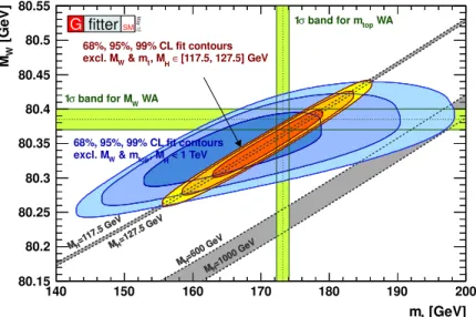
Model have been determined. Figure 2.2 shows a comparison of the world–average of
the measurements of the W boson and top quark masses, m W and m t , with indirect
determinations from the global fit of all Standard Model parameters to the electroweak
precision measurements except m W and m t [33] under different assumptions on the Higgs
boson mass range. The predicted relationship of the W boson and top quark masses are
also shown for different Higgs boson mass scenarios.
2.2. The Minimal Supersymmetric Standard Model 15
[GeV]
m
t140 150 160 170 180 190 200
[GeV]
WM
80.15 80.2 80.25 80.3 80.35 80.4 80.45 80.5 80.55
=117.5 GeV MH =127.5 GeV
MH
=600 GeV MH =1000 GeV
MH
top WA band for m 1σ
W WA band for M 1σ
68%, 95%, 99% CL fit contours < 1 TeV , MH
& mtop
excl. MW
68%, 95%, 99% CL fit contours [117.5, 127.5] GeV
∈ , MH
& mt
excl. MW
=117.5 GeV MH =127.5 GeV
MH
=600 GeV MH =1000 GeV
MH
G fitter
SMMay 12
Figure 2.2: Comparison of the world–average of the measurements of m
Wand m
t(green bands) and the indirect determinations from the global fit to the electroweak precision mea- surements expect m
Wand m
tfor two assumptions on the Higgs boson mass, m
H< 1 TeV (blue area) and 117.5 GeV < m
H< 127.5 GeV (red/yellow area). Also shown is the Standard Model prediction for the relationship of the masses m
Wand m
t, for the two Higgs boson mass scenarios, 117.5 GeV < m
H< 127.5 GeV and 600 GeV < m
H< 1000 GeV (grey bands) [33].
Figure 2.3 shows the pulls of the measured values of individual electroweak observables compared to the corresponding values obtained from the electroweak global fit [34]. The measured values agree with the results of the global fit within two standard deviations, except for the forward–backward asymmetry, A 0,b f b , of b quarks where the two values differ by three standard deviations.
Limitations of the Standard Model
Although the Standard Model is well established by precision tests as a theory describing the known elementary particles and their fundamental interactions at presently accessible energies, there are several open questions which suggest that this model may be only an effective low–energy approximation of a more general theory involving new physics phenomena.
Neutrino Masses In the Standard Model discussed in Section 2.1 it is assumed that
neutrinos are massless. However, the observation of neutrino oscillations [35] requires finite
neutrino masses. Even in simple extensions of the Standard Model which incorporate
neutrino masses [36] there is no explanation why neutrinos are much lighter than the other
fermions.
Measurement Fit |O
meas−O
fit|/σ
meas0 1 2 3
0 1 2 3
∆α
had(m
Z)
∆α
(5)0.02750 ± 0.00033 0.02759 m
Z[GeV]
m
Z[GeV] 91.1875 ± 0.0021 91.1874 Γ
Z[GeV]
Γ
Z[GeV] 2.4952 ± 0.0023 2.4959 σ
had[nb]
σ
041.540 ± 0.037 41.478 R
lR
l20.767 ± 0.025 20.742 A
fbA
0,l0.01714 ± 0.00095 0.01645 A
l(P
τ)
A
l(P
τ) 0.1465 ± 0.0032 0.1481 R
bR
b0.21629 ± 0.00066 0.21579 R
cR
c0.1721 ± 0.0030 0.1723 A
fbA
0,b0.0992 ± 0.0016 0.1038 A
fbA
0,c0.0707 ± 0.0035 0.0742 A
bA
b0.923 ± 0.020 0.935
A
cA
c0.670 ± 0.027 0.668
A
l(SLD)
A
l(SLD) 0.1513 ± 0.0021 0.1481 sin
2θ
effsin
2θ
lept(Q
fb) 0.2324 ± 0.0012 0.2314 m
W[GeV]
m
W[GeV] 80.385 ± 0.015 80.377 Γ
W[GeV]
Γ
W[GeV] 2.085 ± 0.042 2.092 m
t[GeV]
m
t[GeV] 173.20 ± 0.90 173.26
March 2012
![Figure 2.3: Measured values of electroweak observables compared to the corresponding results of the electroweak global fit [34].](https://thumb-eu.123doks.com/thumbv2/1library_info/4019626.1541684/30.892.266.566.153.517/figure-measured-electroweak-observables-compared-corresponding-results-electroweak.webp)
![Figure 2.4: Running of the inverse gauge couplings of the electromagnetic (U (1)), weak (SU (2)) and strong (SU (3)) interactions in the Standard Model (dashed lines) and in the MSSM (solid lines) [4]](https://thumb-eu.123doks.com/thumbv2/1library_info/4019626.1541684/32.892.226.609.298.606/figure-running-inverse-couplings-electromagnetic-strong-interactions-standard.webp)
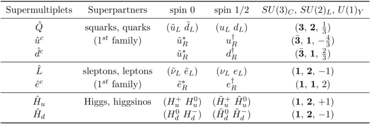
![Table 2.1: Gauge supermultiplets and superpartners in the MSSM and their quantum numbers [3, 4]](https://thumb-eu.123doks.com/thumbv2/1library_info/4019626.1541684/33.892.174.778.801.902/table-gauge-supermultiplets-superpartners-mssm-their-quantum-numbers.webp)
![Table 2.3: Gauge eigenstates of MSSM particles and their corresponding mass eigenstates [4].](https://thumb-eu.123doks.com/thumbv2/1library_info/4019626.1541684/37.892.230.724.323.506/table-gauge-eigenstates-mssm-particles-corresponding-mass-eigenstates.webp)
![Figure 3.5: Decay branching fractions (a) and total width (b) of the Standard Model Higgs boson as a function of its mass, M H [69].](https://thumb-eu.123doks.com/thumbv2/1library_info/4019626.1541684/47.892.168.791.592.909/figure-decay-branching-fractions-standard-model-higgs-function.webp)
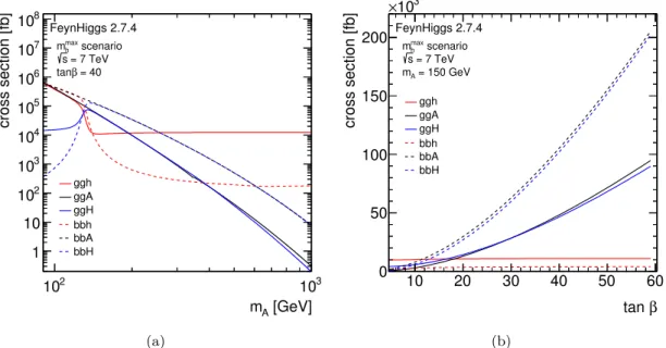
![Figure 3.9: Natural widths of the neutral MSSM Higgs bosons as a function of the mass of the CP–odd Higgs boson, m A , for tan β = 40 (a) and as a function of tan β for m A = 150 GeV (b) calculated in the m max h scenario with FeynHiggs 2.7.4 [59, 62–64].](https://thumb-eu.123doks.com/thumbv2/1library_info/4019626.1541684/51.892.172.779.609.927/figure-natural-neutral-function-function-calculated-scenario-feynhiggs.webp)
