s NN = 5.02 TeV with ATLAS

ATLAS-CONF-2015-054 28September2015

ATLAS NOTE

ATLAS-CONF-2015-054

26th September 2015

Femtoscopy with identified charged pions in proton-lead collisions at √

s NN = 5.02 TeV with ATLAS

The ATLAS Collaboration

Abstract

Bose-Einstein correlations between identified charged pions are measured for

p+Pb colli-

sions at

√

s_NN =

5.02 TeV with the ATLAS detector with a total integrated luminosity of 28 nb

⁻¹

. Pions are identified using ionisation energy loss measured in the pixel detector.

Two-particle correlation functions and the extracted source radii are presented as a func- tion of average transverse pair momentum (k

T

) and collision centrality. Pairs are selected with a pseudorapidity between -1.5 and 1.5 and with an average transverse momentum 0.1

< k_T <

0.8 GeV. The e

ff

ect on the two-particle correlation function from jet frag- mentation is studied, and a new method for constraining its contributions to the measured correlations is described. The measured source sizes are substantially larger in more central collisions and are observed to decrease with increasing pair

k_T

. Linear scaling of the volume with the average multiplicity in the acceptance region

|η| <

1.5 is observed. The scaling of the extracted radii with the mean number of participants is also used to compare a selection of initial-geometry models.

c

2015 CERN for the benefit of the ATLAS Collaboration.

Reproduction of this article or parts of it is allowed as specified in the CC-BY-3.0 license.

1 Introduction

While hydrodynamic models are applied successfully to nucleus-nucleus (A+A) collisions, the extent to which they can describe

p+

Pb collisions remains a topic of active debate. Femtoscopy, the method of using final-state interactions to probe the space-time extent of a particle-emitting source, provides important input to this discussion [1].

Correlation functions of outgoing particle pairs are often studied in A

+

A collisions as a function of rel- ative pseudorapidity (

∆η) and azimuthal angle (∆φ). For |∆η| &

2 the jet contribution does not appear, and the correlation function

C(∆η,∆φ) is then seen to be independent of∆η

[2–7]. These long-range correlations are known as the “ridge”. The pair production is often decomposed into Fourier modes:

dN/d∆φ∼

1

+

2

Σ_nvn

(p

^a_T

)v

n

(

p^b_T

) cos(n∆φ). The measured

vn

components are consistent with hydrody- namic evolution.

Recent observations of the ridge in

p+

Pb [8–10] and

pp

[11, 12] collisions, where the system size is much smaller than in Pb+Pb, raise questions over the interpretation of the

vn

as being purely of hydrodynamic origin. Both hydrodynamic [13–16] and initial-state [17–21] models, as well as a hybrid scenario [22], are able to describe the observed

v₂

and

v₃

in

p+

Pb collisions.

The Hanbury Brown and Twiss (often abbreviated as “HBT”) method originated in astronomy [23, 24], where space-time correlations of photons due to wavefunction symmetrisation are used to measure the size of distant stars. The procedure can be adapted to the tiny sources encountered in hadronic colli- sions if identical-particle Bose-Einstein correlations are instead studied in relative momentum space [25].

Measurements of these Bose-Einstein correlations in

pp

collisions at

√

s =

0.9 GeV and

√

s =

7 GeV have been produced by ATLAS [26], CMS [27], and ALICE [28]. At both energies the source radii are observed to decrease with rising transverse pair momentum

k_T

. It is also observed that the radii increase with particle multiplicity but saturate at the highest multiplicities.

Although Bose-Einstein correlations are the most straightforward to measure experimentally, any non- trivial interaction can be used in principle to image the source density. The term

femtoscopy

is often used to refer to any measurement that provides spatio-temporal information about a hadronic source [29].

The measured source radii are interpreted as the dimensions of a nuclear source at freeze-out, after all interactions between final-state particles and the bulk have ceased; thus, they are sensitive to the space- time evolution of the event. In particular, an increase in radii at low momentum indicates radial expansion since higher momentum particles are more likely to be produced earlier in the event [30]. The results of femtoscopic measurements in

p+Pb systems are of significant interest because they can provide insight

into the extent to which hydrodynamics applies in such small systems. While femtoscopic methods have already been applied to

p+Pb systems at the LHC [31,

32], this analysis presents new data-driven techniques to constrain the significant background contribution from jet fragmentation, referred to in this note as the “hard process” background.

The results presented in this analysis are shown for collision centralities ranging from 0% to 80%, in

centrality intervals no greater than 10% (see Sect. 3.1 for centrality definition). For a pair’s average

four-momentum

k

, the pair pseudorapidity

η_k

is selected from

|η_k| <

1.5 and the results are shown as

a function of transverse pair momentum 0.1 GeV

< k_T <

0.8 GeV. One- and three-dimensional source

radii are presented as a function of the average charged-particle multiplicity, and the scaling of the system

size with the number of initial nucleon participants is also investigated, using the predictions of three

initial-geometry models.

2 ATLAS detector

The ATLAS detector is described in detail in Ref. [33]. The inner detector (ID), which is immersed in a 2 Tesla axial magnetic field, is used to reconstruct charged particles within

|η| <

2.5

1

. It consists of a silicon pixel detector, a semi-conductor tracker (SCT) made of double-layered silicon microstrips, and a transition radiation tracker made of straw tubes. A particle travelling from the interaction point with

|η| <

2 crosses at least 3 pixel layers, 4 double-sided micro-strip layers and typically 36 straw tubes.

The forward calorimeter (FCal), covering a pseudorapidity region of 3.1

< |η| <

4.9, is used to measure the centrality of each collision. The FCal uses liquid argon as the active medium with tungsten and copper absorbers.

The Minimum Bias Trigger Scintillators (MBTS), consisting of two arrays of scintillation counters, are positioned at

z =±3.6 m and cover 2.1 < |η| <

3.9. They are used for the MinBias Level-1 trigger [34]

as well as to impose a constraint on the event selection.

3 Data analysis

3.1 Event and track selection

This analysis uses data from the LHC 2013

p+Pb run at √

s_NN =

5.02 TeV with an integrated luminosity of 28.1 nb

⁻¹

. The Pb ions had an energy per nucleon of 1.57 TeV and collided with the 4 TeV proton beam to yield a centre-of-mass energy

√

s_NN =

5.02 TeV with a longitudinal rapidity boost of 0.465 in the proton direction relative to the ATLAS laboratory frame. Events are required to satisfy the Level-1 MinBias trigger and to have a hit on each side of the MBTS. The di

ff

erence in time between the activity in each side can be no greater than 10 ns. Only a single reconstructed primary vertex (PV) is allowed, which is required to have at least two good tracks. Events which have more than one reconstructed vertex (including secondary vertices) with either more than 10 tracks or a scalar sum of track

p_T

greater than 6 GeV are rejected.

Event centrality is determined following the procedure in Ref. [35], using the total transverse energy in the Pb-going side of the FCal. The use of the FCal for measuring centrality has the advantage that it is not sensitive to multiplicity fluctuations in the kinematic region covered by the inner detector, where the fem- toscopic measurement is performed. For each centrality interval the average charged-particle multiplicity

hd N_ch/dηi

is measured and the corresponding average number of participating nucleons

hN_parti

is derived using methods and data also described in Ref. [35]. Since this analysis uses finer centrality intervals (no wider than 10%), a linear interpolation is used to construct new values based on the published results.

The values and errors from this procedure are tabulated in Sect. 6.2.

Reconstructed tracks, taken from

|η|<

2.5 at

p_T >

0.1 GeV, must originate from hits near the interaction point. A minimum of one pixel hit is required, and if the track crosses an active module in the innermost layer, a hit in that layer is required. For a track

p_T

greater than 0.1, 0.2, or 0.3 GeV there must be at least 2, 4, or 6 hits in the SCT, respectively. The transverse impact parameter with respect to the primary vertex,

1ATLAS uses a right-handed coordinate system with its origin at the nominal interaction point (IP) in the centre of the detector and thez-axis along the beam pipe. The x-axis points from the IP to the centre of the LHC ring, and the y-axis points upward. Cylindrical coordinates (r, φ) are used in the transverse plane,φbeing the azimuthal angle around the beam pipe.

The pseudorapidity is defined in terms of the polar angleθasη=−ln tan(θ/2).

d^PV₀

, must be such that

|d₀^PV| <

1.5 mm. The corresponding longitudinal impact parameter must satisfy

|z^PV₀

sin

θ| <

1.5 mm. Neither

|d₀^PV|

nor

|z^PV₀

sin

θ|

can be larger than 3 times its uncertainty as derived from the covariance matrix of the track parameter fit.

3.2 Particle identification

Particle identification (PID) is performed through measurements of the energy loss

dE/dx

acquired from the ionization charge deposited in the pixel clusters crossed by a track. Relative likelihoods that the track is a

π, K

, and

p

are formed by fitting the

dE/dx

distributions to

√

s =

7 TeV

pp

data in several momentum intervals [36]. Three PID selection levels are defined: one designed to have a high efficiency for pions, one designed to result in high purity, and a middle ground which was chosen as the nominal selection level. The e

ffi

ciency and purity of these selections are studied in a

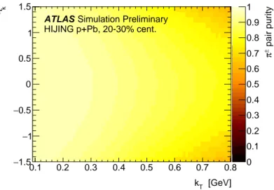
p+

Pb sample generated using Hijing [37] and simulated with the GEANT4 package [38]. The sample is reconstructed with the same conditions as the data. The resulting purity of pairs in the nominal selection is shown in Fig. 1. The results are also evaluated at the looser and tighter PID definitions, and the variation is incorporated into the systematic uncertainty.

[GeV]

kT

0.1 0.2 0.3 0.4 0.5 0.6 0.7 0.8

kη

−1.5

−1

−0.5 0 0.5 1 1.5

pair purity±π

0 0.1 0.2 0.3 0.4 0.5 0.6 0.7 0.8 0.9 1 Simulation Preliminary

ATLAS

HIJING p+Pb, 20-30% cent.

Figure 1: Purity of identified pion pairs, from fully simulated Hijingp+Pb events, as a function of the pair’s average transverse momentumk_Tand pseudorapidityη_k.

3.3 Pair selection

Track pairs are required to have

|∆φ| < π/2 to avoid an enhancement in the correlation function arising

primarily from dijets. This enhancement is not present in the signal region but can influence the results by a

ff

ecting the overall normalization factor in the fits. For a pair’s average momentum

k = ¹₂

p^a+p^b

the pseudorapidity

η_k

must lie inside

|η_k| <

1.5 (a narrower window than the track selection of

|η| <

2.5). When analyzing track pairs of opposite sign, selections on the invariant mass are applied such that

m_ππ−m_ρ0

>

150 MeV,

m_ππ−m_K0 S

>

20 MeV, and

m_{K K} −m_φ(1020)

>

20 MeV, where

m_ab

is

the pair’s invariant mass calculated with particle masses

m_a

and

m_b

. These selections are applied when

forming both the same- and mixed-event distributions.

3.4 Correlation function

The two-particle correlation function is defined as the ratio of two-particle and single-particle momentum spectra:

C p^a,p^b

≡

dN^{a b} d³p^ad³p^b dN^a d³p^a

dN^b d³p^b

,

(1)

for pairs of particles with four-momenta

p^a

and

p^b

. Utilising the correlation function as defined in this way has the experimental advantage that most of the single-particle e

ffi

ciency, acceptance, and resolution effects cancel in the ratio.

It is of physical interest to evaluate the correlation function as a function of the relative momentum

2 q ≡ p^a −p^b

in intervals of average momentum

k ≡ ¹₂

p^a+p^b

. The relative momentum distribution

A(q) ≡ ^dN_dq

^same

is formed by selecting pairs of particles from each event in an event class, which is defined by the collision centrality and

z

position of the primary vertex. The background

B(q) ≡ ^dN_dq

^mix

is constructed by event mixing, that is, by selecting one particle from each of two events in the same event class as

A(q). The ratio of the distributions defines the correlation function:

C_k

(q)

≡ A_k

(q)

B_k

(q)

.

(2)

The relative momentum correlation functions are studied as a function of

q_inv ≡ p

−q_µq^µ

and the three- vector

q. When working in all three dimensions, a longitudinally co-moving frame (LCMF) with the pair

of particles is used such that

k_z =

0. The coordinate axes are defined according to the “out-side-long”

convention [39–41]:

q_out ≡k_T ·q

|k_T| = |p^a_T|²− |p_T^b|²

2k

T

,

(3)

q_side ≡

(ˆ

z×k_T

)

·q

|k_T| =−

ˆ

z·

p^a_T ×p_T^b

k_T ,

(4)

q_long ≡ˆz·q= p_z^aE^b−p_z^bE^a q

k₀²−k²_z

.

(5)

2Whileqhere refers to the relative four-momentum, it is also used generically to refer to either the Lorentz invariantq_invor three-vectorq. The correlation function is studied in terms of both these variables but the description of the analysis is nearly identical for both cases.

3.5 Parameterization and fitting of the correlation function

In the approximation that all particles are identical pions created in a fully chaotic source and that they have no final-state interactions, the correlation function is enhanced by the Fourier transform of the source density. This description is useful for guiding intuition, but is not sufficient for a complete analysis. The Bowler-Sinyukov formalism [42, 43] is used to account for final-state corrections:

C_k

(

q) =

(1

−λ)+λK

(q)C

BE

(q)

,

(6) where

K

is a factor for final-state corrections, and

C_BE

(q)

=

1

+F

[S

k

] (q) with

F

[S

k

] (q) denoting the Fourier transform of the two-particle source density function

S_k

(r ). A number of factors influences the value of the experimental parameter

λ, which is constrained between 0 and 1. Including non-identical

particles decreases this parameter, as does coherent emission. Products of weak decays or long-lived resonances are emitted at a length scale greater than can be resolved by the momentum resolution of the detector, and also lead to a decrease in

λ. These additional contributions to the source density are not

Coulomb-corrected in the Bowler-Sinyukov form. When describing pion pairs of opposite charge, there is no Bose-Einstein enhancement and

C_BE →

1.

The particular choice of the correction factor

K(q) is determined using the formalism in Ref. [44], under

the approximation that the Coulomb correction is e

ff

ectively applied over a Gaussian source density of radius

R_eff

:

K

(q

_inv

)

=G(q_inv

)

"

1

+

8R

_eff

√πa²F₂

1 2

,

1; 3

2

,

3

2 ;

−R²_effq²_inv

!#

,

(7)

where

G(qinv

) is the Gamow factor [45]

G(qinv

)

= _aq^4π_inv e

4π aqinv −

1

−1

,

a =

388 fm is the Bohr radius of two pions, and

2F₂

is a generalised hypergeometric function.

The Bose-Einstein enhancement in the correlation function is fit to an exponential form,

C_BE

(q)

=

1

+e^{− | |Rq| |},

(8)

where

q

refers to either

q_inv

or

q

depending on whether it is applied to the one- or three-dimensional correlation function, and

R

is a diagonal matrix in one or three dimensions whose components are the source radii. The double-bar expression

||Rq||

indicates the vector magnitude of

Rq

in three dimensions and the absolute value of

R_invq_inv

in one dimension. This function corresponds to an underlying Cauchy source density. A Gaussian enhancement is found to not describe the data as well as an exponential, which is also observed in the

pp

results in Ref. [26]. The choice of form for

F

[S

k

](q) must be taken into account when interpreting source radii, and there is no simple correspondence between results using one form and those using another.

A negative log-likelihood ratio

L

is minimised that assumes the bin contents of

A

and

B

are Poisson distributed and

C

is best fit to the ratio of their means:

−2 lnL =

2

X

i

"

A_i

ln (1

+C_i

)

A_i C_i

(

A_i+B_i+

2)

!

+

(B

_i+

2) ln (1

+C_i

)(

B_i+

2)

A_i+B_i +

2

!#

.

(9)

The factor

−2 makes this statistic approach χ²

in the high-statistics limit. Here

A

and

B

are the quantities in Eq. 2 when considered as histograms, such that

A_i

and

B_i

are the contents in bin

i.C_i

is shorthand for

C

(q

i

) where

q_i

is the bin centre and

C(q) is the fitting function describing the correlation. The statistical

uncertainties in the fit parameters of

C

(q) are selected from the points in the parameter space where

−2 lnL=

min (−2 ln

L)+

1.

4 Hard-process contribution

Additional non-femtoscopic enhancements to the correlation functions at

q_inv.

0.5

−

1 GeV are observed in both

+−

(opposite charge) and

±±

(same charge) pairs. This section describes the Monte Carlo (MC) generators used to study these structures and presents the study performed to constrain their description.

4.1 Monte Carlo generators

Four Monte Carlo generator-level samples are used to study the background described in this section at the truth level. No subsequent simulation is performed, as the effects of the reconstruction were studied using full simulation and found to be negligible. In each of the following samples, 50 million minimum-bias events are generated at a centre-of-mass energy per nucleon-nucleon pair of

√

s_NN =

5.02 TeV.

1. H

ijingp+

Pb [37]

The same settings as in the nominal ATLAS

p+

Pb reconstructed simulation (as described in Sect. 3.2) are used, except that the minimum hard-scattering

p_T

is adjusted as described in Sect. 4.2. A boost is applied along the collision axis in the proton-going direction to match the frame of the measured

p+

Pb system.

2. H

ijingpp

The generator is run with all of the same settings as the

p+

Pb sample, except that both incoming particles are protons and no boost is applied.

3. P

ythia

8

pp

[46]

The default ATLAS tune “UE AU2-CTEQ6L1” is used with P

ythia

8.209, which utilises the CTEQ 6L1 parton distribution function (PDF) from LHAPDF6 [47].

4. H

erwig++pp

[48]

The NNLO MRST PDF [49] was used with H

erwig++

2.7.1.

4.2 Data-driven estimate of hard process backgrounds

The non-femtoscopic enhancement is more prominent at higher

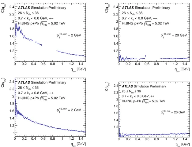
k_T

and lower multiplicities. This suggests that the correlation is primarily due to jet fragmentation. This attribution is verified by studying corre- lation functions in Hijing where the contribution from jets can be removed by increasing the minimum hard-scattering

p_T

from 2 to 20 GeV, as demonstrated in Fig. 2.

The amplitude of the hard-process contribution tends to be larger in Monte Carlo generators than it is

in the data. Thus, attempting to account for it by studying the double-ratio

C^data

(

q)/C^MC

(q) leads to a

depletion that is apparent in the region where the Bose-Einstein enhancement disappears [26]. Another

[GeV]

qinv

0 0.2 0.4 0.6 0.8 1 1.2 1.4

) invC(q

1 1.2 1.4 1.6 1.8 2 2.2

2.4 ATLAS Simulation Preliminary

≤ 36 Nch

≤ 26

− + < 0.8 GeV, 0.7 < kT

= 5.02 TeV sNN

HIJING p+Pb

= 2 GeV

HS, min

pT

[GeV]

qinv

0 0.2 0.4 0.6 0.8 1 1.2 1.4

) invC(q

1 1.2 1.4 1.6 1.8 2 2.2

2.4 ATLAS Simulation Preliminary

≤ 36 Nch

≤ 26

− + < 0.8 GeV, 0.7 < kT

= 5.02 TeV sNN

HIJING p+Pb

= 20 GeV

HS, min

pT

[GeV]

qinv

0 0.2 0.4 0.6 0.8 1 1.2 1.4

) invC(q

1 1.2 1.4 1.6 1.8 2 2.2

2.4 ATLAS Simulation Preliminary

≤ 36 Nch

≤ 26

+ + < 0.8 GeV, 0.7 < kT

= 5.02 TeV sNN

HIJING p+Pb

= 2 GeV

HS, min

pT

[GeV]

qinv

0 0.2 0.4 0.6 0.8 1 1.2 1.4

) invC(q

1 1.2 1.4 1.6 1.8 2 2.2

2.4 ATLAS Simulation Preliminary

≤ 36 Nch

≤ 26

+ + < 0.8 GeV, 0.7 < kT

= 5.02 TeV sNN

HIJING p+Pb

= 20 GeV

HS, min

pT

Figure 2: Correlation functions of truth-level charged particles from Hijingfor+−pairs (top) and++pairs (bottom).

The generator is run with the minimum hard-scatteringp^{HS, min}_T at the default setting of 2 GeV (left) and turned up to 20 GeV (right) to remove the contribution from hard processes. The gaps in the opposite-sign correlation functions are a result of the selections described in Sect.3.3, which remove the largest resonance contributions.

commonly used method is to parameterize the mini-jet contribution using MC and allow one or more parameters of the description to be free in the fit [31, 32].

The analysis presented in this note avoids both of these strategies and instead develops a data-driven method to constrain the correlations from jet fragmentation. Opposite-sign correlation functions are used to predict the jet contribution in the same-sign correlation function. This has two clear di

ffi

culties. Firstly, resonance decays appear prominently in the opposite-sign correlations. The most prominent of these are removed by selections on the invariant mass of the opposite-sign pairs (as described in Sect. 3.3), and the fits ignore opposite-sign structure below

q_inv=

0.2 GeV. Secondly, jet fragmentation a

ff

ects the opposite- sign correlations at a different level than it does for same-sign pairs. This is in part because opposite-sign pairs are more likely to have a closer common ancestor in a jet’s fragmentation into hadrons.

To account for the remaining differences between

+−

and

±±

pairs, a study of the correlation function comparison is performed in P

ythia

8. H

ijing

, which uses P

ythia

6, was found to describe the charge comparison inadequately. Fits are performed to a stretched exponential function of the form

C

(q

inv

)

=N

1

+λbkgde^{− |Rbkgdqinv|αbkgd}

,

(10)

where

N

is a normalization factor and the other parameters depend on the charge combination and on

k_T

. First,

α_bkgd

is determined with fits to same-sign correlation functions. The fits are well described by a Gaussian form (α

_bkgd=

2) at

k_T .

0.4 GeV. The shape parameter

α_bkgd

is only very weakly dependent on multiplicity, so a function is fit to parameterize

α_bkgd

as a function of

k_T

. The fits to correlation functions are performed again with

α_bkgd

fixed to the same value in same- and opposite-charged pairs, and a comparison is made between the width parameters

R_bkgd⁺⁻

and

R^±±_bkgd

. The width of the jet fragmentation correlation for same-sign pairs is found to be roughly proportional to that for opposite-sign pairs:

R_bkgd^±± = ρR⁺_bkgd⁻ .

(11) This proportionality begins to break down at low

k_T

, but in this kinematic region hard processes contribute little to the correlation function (i.e.

λ_bkgd

is small). The multiplicity of charged particles,

N_ch

, is the number of truth-level charged particles for

p_T >

0.1 GeV and

|η| <

2.5. The

ρ

parameter is extracted as a

k_T

- and multiplicity-independent factor. Finally,

R^±±_bkgd

is also fixed from

R_bkgd⁺⁻

using the value of

ρ, and

the fits are performed again to parameterize the relationship between the amplitudes:

λ^±±_bkgd= µ(k_T

)

λ⁺_bkgd⁻ ν(kT)

.

(12)

At each

k_T

,

µ

and

ν

are fit to describe four multiplicity intervals (26

≤ N_ch ≤

36, 37

≤ N_ch ≤

48, 49

≤ N_ch ≤

64, and 65

≤ N_ch

). The power-law scaling of Eq. 12 is found to provide a good description of the relation between the same- and opposite-sign amplitudes across all four multiplicity intervals studied.

The multiplicity-independence of

µ

and

ν

is important to justify the use of these parameters in

p+Pb.

Since this study is done with P

ythia

8 in a

pp

system, H

ijing

is also used to compare the correspondence between opposite- and same-sign pairs in both

pp

and

p+

Pb. While the mapping is mostly consistent between the two systems, it is found that

µ

is larger in

p+Pb than in pp

by 8.5% on average. When the mapping is applied to the data, this factor is also taken into account, and the standard deviation of this factor is incorporated into a systematic uncertainty.

With

α_bkgd

(

k_T

),

µ(k_T

),

ν(k_T

), and

ρ

determined from generator-level samples, the mapping can be applied to the

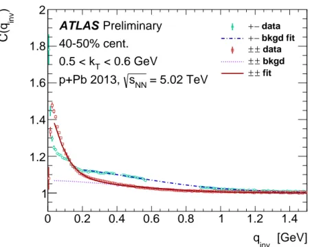
p+

Pb data. As illustrated in Fig. 3, the

+−

correlation function is fit to Eq. 10 for

q_inv >

0.2 GeV, with

α_bkgd

fixed from Pythia 8 and

λ⁺_bkgd⁻

and

R_bkgd⁺⁻

as free parameters. The

µ,ν, and ρ

are used to infer

λ^±±_bkgd

and

R^±±_bkgd

, which are fixed before the femtoscopic part of the correlation function is fit to

±±

data.

In three dimensions,

q_inv

is calculated from

q

and the average

k_T

in each bin. The same parameters used to describe the hard-process contribution in the invariant correlation function are also used in the 3D fit.

The full form of the correlation function fit to

±±

data including the hard-process background description is

C

(q)

=N

1

−λ+λK

(q

_inv

)C

_BE

(q)

1

+λ^±±_bkgde^{− |R±±bkgdqinv|}

αbkgd

,

(13)

where

q

refers generically to either

q_inv

or

q.

[GeV]

q

inv

0 0.2 0.4 0.6 0.8 1 1.2 1.4

)

inv

C(q

1 1.2 1.4 1.6 1.8 2

data

− +

bkgd fit

− +

data

±

± bkgd

±

±

± fit

±

Preliminary ATLAS

40-50% cent.

< 0.6 GeV 0.5 < k

T

= 5.02 TeV s

NN

p+Pb 2013,

Figure 3: Correlation functions inp+Pb data for opposite-sign (teal circles) and same-sign (red squares) pairs. The opposite-sign correlation function, with the most prominent resonances removed, is fit to a function of the form in Eq.10(blue dashed line). The violet dotted line is the estimation of the jet contribution in the same-sign correlation function, also of the form of Eq.10, and the dark red line is the full fit of Eq.13to the same-sign data.

5 Systematic uncertainties

Systematic uncertainties are determined to account for the hard-process background description, PID, the effective Coulomb correction size

R_eff

, charge asymmetry, and two-particle effects.

One of the largest sources of uncertainty in femtoscopy in small systems in high-energy collisions comes from forming an accurate description of the background contribution from hard processes. For the uncer- tainty in the hard-process contribution three effects are considered. The variation in the translation from

pp

to

p+

Pb is taken as an uncertainty in the amplitude, as mentioned in Sect. 4. Additionally, the ampli- tude of

C⁺⁻

(q

inv

)

C^±±

(q

inv

) is studied in both Pythia and Herwig. Herwig predicts not nearly enough difference between

+−

and

±±

to describe the data. Thus, instead of using the ratio between the two generators’ predicted scalings, the standard deviation of the ratio amplitude (across a selection of

k_T

and multiplicity intervals) is used as a systematic variation. The hard-process amplitude

λ_bkgd

is scaled up and down by 12.3%, the quadrature sum of the relative variation from the

pp

to

p+Pb distinction (4.1%) and

from the generator di

ff

erence (11.6%). Additionally, in three-dimensional fits the mini-jet contribution is described by mapping

q

onto

q_inv

, which uses the average

k_T

in the interval. The choice of

k_T

is varied up and down by one standard deviation of the values in that

k_T

interval (typically about 30 MeV).

The analysis is repeated at both a looser and a tighter PID selection definition, and the variation is in-

cluded as a systematic uncertainty. The effect on the radii is at the 1-2% level for the lower

k_T

intervals,

but becomes more significant at higher momentum intervals, where there are relatively more kaons and

protons and the

dE/dx

separation is not as good.

k_T

[GeV] 0.1–0.2 0.2–0.3 0.3–0.4 0.4–0.5 0.5–0.6 0.6–0.7 0.7–0.8

λ_bkgd

3.1% 2.8% 4.4% 5.4% 7.8% 11% 16%

E

ff

ective Coulomb size

R_eff

4.6% 5.2% 5.4% 4.3% 3.9% 3.7% 3.6%

Pion identification 0.1% 0.21% 0.43% 1.3% 1% 3.2% 2.1%

Charge asymmetry 1% 0.37% 0.29% 0.13% 1.3% 2.6% 1.6%

Minimum

q

in fit 0.45% 0.44% 0.98% 0.68% 1.3% 1.5% 0.54%

All 5.6% 5.9% 7.1% 7.1% 9% 12% 16%

Table 1: The relative systematic uncertainties inR_invin the 1-5% centrality interval. The quadrature average of the upper and lower systematic errors is divided by the nominal value to compute the relative uncertainty. The uncer- tainty is dominated by the hard-process background description and the contribution from the effective Coulomb sizeR_effis also significant at lowkT.

k_T

[GeV] 0.1–0.2 0.2–0.3 0.3–0.4 0.4–0.5 0.5–0.6 0.6–0.7 0.7–0.8

λ_bkgd

2% 3.7% 6.6% 9.4% 12% 16% 20%

E

ff

ective Coulomb size

R_eff

1.4% 1.2% 0.98% 0.86% 0.87% 0.83% 0.74%

Pion identification 1.1% 2.7% 4.7% 4.2% 3.8% 4.1% 3.4%

Charge asymmetry 0.66% 0.73% 0.069% 0.83% 0.087% 2.2% 1.8%

Minimum

q

in fit 0.82% 1.2% 1.5% 1.7% 0.71% 0.68% 0.42%

All 2.9% 4.9% 8.3% 11% 13% 16% 20%

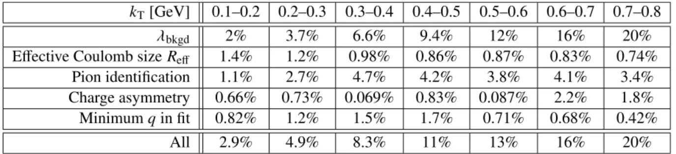
Table 2: The relative systematic uncertainties inRinvfor the 60-70% centrality interval, as in Table1. The uncer- tainty is dominated by the hard-process background description.

The non-zero e

ff

ective size of the Coulomb correction

R_eff

should only provide a bin-by-bin di

ff

erence of a few percent, even with a value up to several fm, since the Bohr radius of pions is nearly 400 fm. However, since the parameter changes the

q_inv

width over which the Coulomb correction is applied, varying this parameter can a

ff

ect the source radii from around 1% (peripheral) to 6% (central). The nominal value of 3 fm lies in the middle of the measured radii. The

R_eff

is varied down to 1 fm and up to 6 fm, and the change in the radii is included in the systematic uncertainties. This range is chosen as a conservative estimate, as it encompasses the majority of the results.

A small difference between positive and negative charge pairs is observed, attributable to detector effects such as the orientation of the overlap of the inner detector component staves. The nominal results use all of the same-sign pairs, and a systematic variation accounting for this charge asymmetry is chosen to overlap the results for both of the separate charge states.

Single-particle correction factors cancel out in the ratio

A(q)/B(q). However, two-particle eff

ects on the track reconstruction can a

ff

ect the correlation function. In the reconstructed H

ijing

sample, the truth-level and reconstructed correlation functions are compared, and a depletion in the first few

q_inv

bins is observed.

A minimum

q

cuto

ff

is applied in the fits to avoid being a

ff

ected by these detector e

ff

ects. The sensitivity of the results to this limit is checked by taking

q^min_inv =

30

±

10 MeV in the 1D fits, and symmetrising the effect of the variation from

|q|^min=

25 to 50 MeV in the 3D fits.

The relative systematic uncertainties in

R_inv

are shown for a central interval (1-5%) in Table 1 and a

peripheral interval (60-70%) in Table 2. The relative systematic uncertainties are also tabulated for the

3D radii

R_out

(Table 3),

R_side

(Table 4), and

R_long

(Table 5) averaged over centrality.

k_T

[GeV] 0.1–0.2 0.2–0.3 0.3–0.4 0.4–0.5 0.5–0.6 0.6–0.7 0.7–0.8

λ_bkgd

2% 3% 4.4% 6.9% 8.2% 9.8% 13%

Effective Coulomb size

R_eff

3.5% 4.2% 4.7% 5.1% 4.5% 3.6% 2.2%

Pion identification 0.51% 1.2% 1.6% 1.5% 1.5% 4.5% 17%

Charge asymmetry 1.4% 1.4% 0.93% 0.87% 1.2% 1.3% 1.1%

Minimum

q

in fit 1.3% 1.4% 0.75% 0.37% 0.17% 0.24% 0.67%

k_T

in background 0.18% 0.89% 0.31% 0.28% 0.17% 0.11% 0.16%

All 5% 6.4% 7.4% 9.2% 9.9% 12% 22%

Table 3: The relative systematic uncertainties inR_out, averaged over centrality. The quadrature average of the upper and lower systematic errors is divided by the central value, which is averaged equally over centrality intervals from 0% to 80%. The values in the “All” row are averaged over centrality in the same way but include all systematic variations added in quadrature.

k_T

[GeV] 0.1–0.2 0.2–0.3 0.3–0.4 0.4–0.5 0.5–0.6 0.6–0.7 0.7–0.8

λ_bkgd

1.6% 2.5% 3.5% 5.3% 6.6% 8.4% 11%

Effective Coulomb size

R_eff

2.5% 2.4% 2.4% 2.3% 2% 2.2% 3.1%

Pion identification 0.25% 0.84% 1.2% 1.4% 1.9% 7.2% 34%

Charge asymmetry 0.97% 0.85% 0.47% 1% 1.4% 1.6% 3%

Minimum

q

in fit 0.47% 0.85% 0.49% 0.33% 0.22% 0.27% 0.93%

k_T

in background 0.045% 0.44% 0.097% 0.11% 0.27% 0.55% 1.2%

All 3.3% 4.1% 4.8% 6.2% 7.4% 12% 36%

Table 4: The relative systematic uncertainties inR_side, averaged over centrality in the same manner as in Table3.

k_T

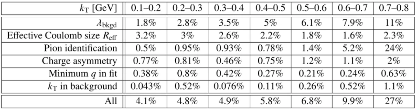
[GeV] 0.1–0.2 0.2–0.3 0.3–0.4 0.4–0.5 0.5–0.6 0.6–0.7 0.7–0.8

λbkgd

1.8% 2.8% 3.5% 5% 6.1% 7.9% 11%

E

ff

ective Coulomb size

R_eff

3.2% 3% 2.6% 2.2% 1.8% 1.6% 2.3%

Pion identification 0.5% 0.95% 0.93% 0.78% 1.4% 5.2% 24%

Charge asymmetry 0.77% 0.81% 0.46% 0.75% 1.2% 1.1% 2%

Minimum

q

in fit 0.38% 0.8% 0.42% 0.27% 0.21% 0.24% 0.63%

k_T

in background 0.043% 0.52% 0.076% 0.11% 0.26% 0.52% 1.1%

All 4.1% 4.8% 4.9% 5.8% 6.8% 9.9% 27%

Table 5: The relative systematic uncertainties inR_long, averaged over centrality in the same manner as in Table3.

6 Results

This section first shows examples of fits to correlation functions and discusses the evaluation of two quantities,

hd N_ch/dηi

and

hN_parti, for each centrality interval. The remainder of the section presents

results for extracted invariant and 3D source radii as a function of

k_T

,

hd N_ch/dηi

, and

hN_parti

.

6.1 Fit examples

An example of a fit to

C(qinv

) was included in Fig. 3, using the functional form of Eq. 13. The fit in the same-sign correlation function reasonably describes the data, although the statistical uncertainties are so small that a small departure of the correlation function from the exponential description can be detected.

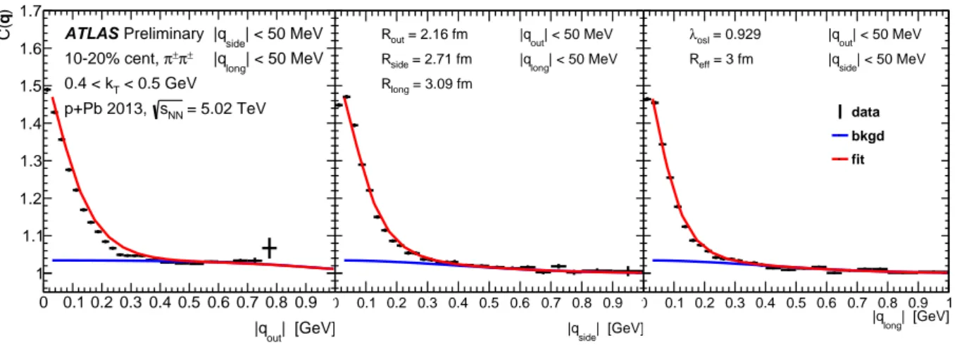
Slices of a three-dimensional (3D) fit of

C(q) to the three-dimensional variant of Eq.

13 are shown in Fig. 4. The apparently imperfect fit along the

q_out

axis is characteristic of

q_side ≈ q_long ≈

0, and away from this slice the agreement of the fit with the data improves.

| [GeV]

|qout

0 0.1 0.2 0.3 0.4 0.5 0.6 0.7 0.8 0.9 1

)qC(

1 1.1 1.2 1.3 1.4 1.5 1.6 1.7

Preliminary ATLAS

π±

π±

10-20% cent, < 0.5 GeV 0.4 < kT

= 5.02 TeV sNN

p+Pb 2013,

| < 50 MeV

|qside

| < 50 MeV

|qlong

| [GeV]

|qside

0 0.1 0.2 0.3 0.4 0.5 0.6 0.7 0.8 0.9 1 1

1.1 1.2 1.3 1.4 1.5 1.6 1.7

= 2.16 fm Rout

= 2.71 fm Rside

= 3.09 fm Rlong

| < 50 MeV

|qout

| < 50 MeV

|qlong

| [GeV]

|qlong

0 0.1 0.2 0.3 0.4 0.5 0.6 0.7 0.8 0.9 1 1

1.1 1.2 1.3 1.4 1.5 1.6 1.7

data bkgd fit = 0.929

λosl

= 3 fm Reff

| < 50 MeV

|qout

| < 50 MeV

|qside

Figure 4: Example of the 3D fit showing slices along each axis inq-space. The blue line indicates the description of the contribution from hard processes and the red line shows the full correlation function fit. The test statistic

−2 lnL=22369 and there are 19805 degrees of freedom in the fit.

6.2 Centrality: N

_part

and average multiplicity

The mean

N_part

(hN

_parti) in each centrality interval is extracted using the procedure in Ref. [35]. The values

used for

hN_parti

are shown in Table 6 for each of the three models evaluated. The Glauber

hN_parti

are also used to perform a linear interpolation for

hd N_ch/dηi

in finer centrality intervals than those available in Ref. [35]. The interpolation is justified with the result in Ref. [35] that charged particle multiplicity is proportional to

hN_parti

in the peripheral region. The average charged particle multiplicities within

|η| <

1.5 that are extracted using this interpolation are also shown in Table 6.

Centrality

hN_parti^Glauber hN_parti^GGCFω_σ =

0.11

hN_parti^GGCFω_σ =

0.2

hd N_ch/dηi

0–1% 18.22

⁺_−1.01^2.62

24.18

⁺_−2.07^1.52

27.42

⁺_−4.48^1.58

58.07

±

0.09

±

1.86 1–5% 16.10

⁺_−0.90^1.66

19.52

⁺_−1.32^1.24

21.41

⁺_−1.98^1.46

45.78

±

0.09

±

1.33 5–10% 14.61

⁺_−0.82^1.21

16.49

⁺_−1.00^1.00

17.46

⁺_−1.08^1.13

38.53

±

0.06

±

1.12 10–20% 13.05

⁺_−0.73^0.82

13.77

⁺_−0.81^0.79

14.11

⁺_−0.79^0.86

32.34

±

0.05

±

0.97 20–30% 11.37

⁺_−0.63^0.65

11.23

⁺_−0.67^0.62

11.17

⁺_−0.62^0.68

26.74

±

0.04

±

0.80 30–40% 9.81

⁺_−0.57^0.56

9.22

⁺_−0.54^0.50

8.97

⁺_−0.49^0.60

22.48

±

0.03

±

0.75 40–50% 8.23

⁺_−0.55^0.48

7.46

⁺_−0.43^0.41

7.15

⁺_−0.39^0.54

18.79

±

0.02

±

0.69 50–60% 6.64

^+0.41_−0.52

5.90

^+0.36_−0.34

5.60

^+0.47_−0.30

15.02

±

0.02

±

0.62 60–70% 5.14

^+0.35_−0.43

4.56

^+0.32_−0.26

4.32

^+0.41_−0.23

11.45

±

0.01

±

0.56 70–80% 3.90

^+0.24_−0.30

3.5

^+0.22_−0.18

3.34

⁺_−0.16^0.29

8.49

±

0.02

±

0.51

Table 6:hN_partifor each centrality interval in the Glauber model as well as the two choices for the Glauber-Gribov model with colour fluctuations (GGCF), along with the average multiplicity within|η|<1.5. Asymmetric system- atic uncertainties are shown forhN_parti. The uncertainties inhd N_ch/dηiare given in the order of statistical followed by systematic.

6.3 One-dimensional results

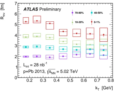
The results from fits of

C(qinv

) to Eq. 13 for the invariant radius

R_inv

are shown in Fig. 5 in four selected centrality intervals. The clear decrease in size with increasing

k_T

that is observed in central events is not significant in peripheral events. Taken at face value, this suggests that central events undergo transverse expansion, since in hydrodynamic models higher-p

T

particles are more likely to freeze out earlier in the event. Another way of understanding this trend as evidence for transverse expansion is that there is a smaller homogeneity region for particles with higher

p_T

[30]. At low

k_T

, ultra-central (0-1%) events have an invariant radius significantly greater than peripheral (70-80%) events by a factor of about 2.6. This difference becomes less prominent at high

k_T

.

Invariant radii are also shown for all centralities in Fig. 6, as a function of the cube root of average

d N_ch/dη. For both k_T

intervals shown, the scaling of

R_inv

with

hd N_ch/dηi^1/3

is close to linear but with

a slightly increasing slope at higher multiplicities.

R_inv

has a steeper trend versus multiplicity at lower

k_T

.

[GeV]

kT

0.2 0.3 0.4 0.5 0.6 0.7 0.8

[fm]invR

0 1 2 3 4 5 6 7

70-80% 40-50%

10-20% 0-1%

Preliminary ATLAS

= 5.02 TeV sNN

p+Pb 2013, = 28 nb-1

Lint

Figure 5: The exponential invariant radiiR_invas a function ofk_T. The vertical sizes of the boxes are the quadrature sum of the systematic uncertainties described in Sect.5, and statistical uncertainties are shown with vertical lines.

The horizontal positions of the boxes are the averagek_Tin each interval, and the widths of the boxes indicate the standard deviation ofkT.

>1/3

η

ch/d

<dN

2 2.5 3 3.5 4

[fm]invR

0 1 2 3 4 5 6 7

< 0.3 GeV 0.2 < kT

< 0.6 GeV 0.5 < kT

= 5.02 TeV sNN

p+Pb 2013, = 28 nb-1

Lint

Preliminary ATLAS

Figure 6: Exponential fit results for Rinvas a function of the cube root of average charged particle multiplicity, hd N_ch/dηi^1/3, where the average is taken over |η| < 1.5. The systematic uncertainties from the background amplitude and pion identification are shown as error bands while the systematics from charge asymmetry, R_eff, andq-cutoffare indicated by the height of the boxes. The horizontal error bars indicate the systematic uncertainty fromhd N_ch/dηias tabulated in Sect.6.2.

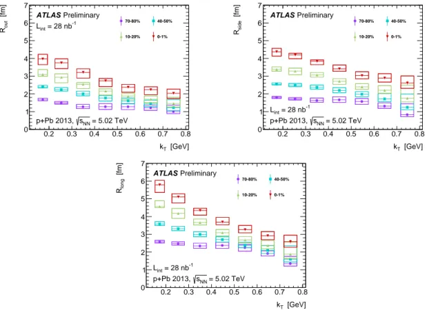
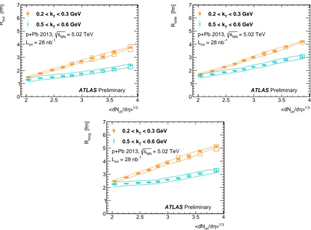
6.4 Three-dimensional results

The three-dimensional radii

R_out

,

R_side

, and

R_long

are shown as a function of

k_T

in a selection of four centrality intervals in Fig. 7. The 3D radii exhibit an even steeper drop-o

ff

from low to high

k_T

in central events relative to what is observed for the invariant radii in Fig. 5. This trend is present, but not as strong, in peripheral events.

The radii are also shown as a function of the cube root of average multiplicity in Fig. 8, which probes the relationship between the size and the source density at freeze-out. Linear scaling is observed with di

ff

erent intercepts at di

ff

erent values of

k_T

, in a qualitatively similar way to the scaling of

R_inv

with

hd N_ch/dηi

in Fig. 6.

[GeV]

kT

0.2 0.3 0.4 0.5 0.6 0.7 0.8

[fm]outR

0 1 2 3 4 5 6 7

70-80% 40-50%

10-20% 0-1%

Preliminary ATLAS

= 5.02 TeV sNN

p+Pb 2013, = 28 nb-1

Lint

[GeV]

kT

0.2 0.3 0.4 0.5 0.6 0.7 0.8

[fm]sideR

0 1 2 3 4 5 6 7

70-80% 40-50%

10-20% 0-1%

Preliminary ATLAS

= 5.02 TeV sNN

p+Pb 2013, = 28 nb-1

Lint

[GeV]

kT

0.2 0.3 0.4 0.5 0.6 0.7 0.8

[fm]longR

0 1 2 3 4 5 6 7

70-80% 40-50%

10-20% 0-1%

Preliminary ATLAS

= 5.02 TeV sNN

p+Pb 2013, = 28 nb-1

Lint

Figure 7: Exponential fit results for 3D source radii as a function ofk_T. A selection of four non-adjacent centrality intervals are shown. The vertical size of the boxes are the quadrature sum of the systematic uncertainties described in Sect.5, and statistical uncertainties are shown with vertical lines. The horizontal positions of the boxes are the averagek_Tin each interval, and the widths of the boxes indicate the standard deviation ofk_T.

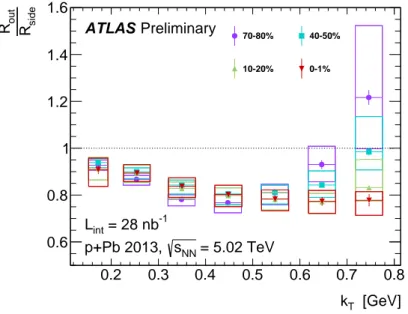
The ratio

R_out/R_side

(Fig. 9) is often of interest since, in models with radial flow,

R_out

includes components of the source’s lifetime but

R_side

does not (see, for instance, the discussion in [1]). A value of

R_out/Rside

less than 1 is observed with a decrease at increasing

k_T

. In the region where the systematic uncertainties

are small, the ratio is observed to remain constant over centrality. As explained in [50], several improve-

ments to naive hydrodynamic models—primarily pre-thermal acceleration, a sti

ff

er equation of state, and

shear viscosity—all result in more sudden emission. Thus, a value of

R_out/R_side .

1 does not necessarily

rule out collective behaviour.

>1/3

η

ch/d

<dN

2 2.5 3 3.5 4

[fm]outR

0 1 2 3 4 5 6 7

< 0.3 GeV 0.2 < kT

< 0.6 GeV 0.5 < kT

= 5.02 TeV sNN

p+Pb 2013, = 28 nb-1

Lint

Preliminary ATLAS

>1/3

η

ch/d

<dN

2 2.5 3 3.5 4

[fm]sideR

0 1 2 3 4 5 6 7

< 0.3 GeV 0.2 < kT

< 0.6 GeV 0.5 < kT

= 5.02 TeV sNN

p+Pb 2013, = 28 nb-1

Lint

Preliminary ATLAS

>1/3

η

ch/d

<dN

2 2.5 3 3.5 4

[fm]longR

0 1 2 3 4 5 6 7

< 0.3 GeV 0.2 < kT

< 0.6 GeV 0.5 < kT

= 5.02 TeV sNN

p+Pb 2013, = 28 nb-1

Lint

Preliminary ATLAS

Figure 8: The scaling of the 3D exponential radii with the cube root of charged-particle multiplicity. Systematic uncertainties from the hard-process description and pion identification are shown in bands while those from charge asymmetry,R_eff, and the minimum cutoffin the fits are represented by the height of the boxes. Statistical uncer- tainties are included but are smaller than the markers. The horizontal error bars indicate the systematic uncertainty fromhd N_ch/dηias tabulated in Sect.6.2.

[GeV]

kT

0.2 0.3 0.4 0.5 0.6 0.7 0.8

sideR

outR

0.6 0.8 1 1.2 1.4 1.6

70-80% 40-50%

10-20% 0-1%

Preliminary ATLAS

= 5.02 TeV sNN

p+Pb 2013, = 28 nb-1

Lint

Figure 9: The ratio of exponential radii R_out/R_side as a function of k_T. The vertical size of the boxes are the quadrature sum of the systematic uncertainties described in Sect.5, and statistical uncertainties are shown with vertical lines. The horizontal positions of the boxes are the averagek_Tin each interval, and the widths of the boxes indicate the standard deviation ofk_T.

η>

ch/d

<dN

0 10 20 30 40 50 60

]3 [fmlong Rside RoutR

0 10 20 30 40 50 60 70 80 90

< 0.3 GeV 0.2 < kT

< 0.6 GeV 0.5 < kT

= 5.02 TeV sNN

p+Pb 2013, = 28 nb-1

Lint

Preliminary ATLAS

Figure 10: The productR_outR_sideR_longfor twok_Tintervals plotted against the average multiplicity. The systematic uncertainties from the background description and pion identification are shown as error bands while the systematic uncertainties from charge asymmetry, R_eff, andq-cutoffare indicated by the height of the boxes. The horizontal error bars indicate the systematic uncertainty fromhd N_ch/dηias tabulated in Sect.6.2.

part>

<N

0 5 10 15 20 25 30

]3 [fmlong Rside RoutR

0 10 20 30 40 50 60 70 80 90

= 0) ωσ

Glauber ( = 0.11 ωσ

GGCF

= 0.2 ωσ

GGCF

= 5.02 TeV sNN

p+Pb 2013,

< 0.3 GeV 0.2 < kT

Preliminary ATLAS

Figure 11: The scaling of the productR_outR_sideR_long withhN_parti calculated with three initial geometry models:

standard Glauber as well as Glauber-Gribov (GGCF) for two choices of the colour fluctuation parameterω_σ. The systematic uncertainties from the background description and pion identification are shown as error bands while the systematics from charge asymmetry,R_eff, andq-cutoffare indicated by the height of the boxes. The horizontal error bars indicate the systematic uncertainties inhN_partias tabulated in Sect.6.2.

The product of 3D radius parameters,

R_outR_sideR_long

, is shown in Fig. 10 as a function of the average multiplicity. The scaling of the volume with the multiplicity is nearly linear, which implies a constant freeze-out density. Fig. 11 compares the volume scaling with

hN_parti

for the standard Glauber model as well as for two choices of the Glauber-Gribov colour fluctuation (GGCF) model [51]. The parameter

ω_σ

controls fluctuations in the nucleon-nucleon cross section within the Glauber-Gribov model. It is observed that a model that includes non-zero fluctuations in the proton size must be used in order to maintain a linear scaling of the volume with

hN_parti. Atk_T >

0.6 GeV, this linear scaling no longer holds even for the

ω_σ =

0.2 model. The values and systematic uncertainties for

hN_parti

in each model are listed in Sect. 6.2.

7 Summary and conclusions

Bose-Einstein correlations of identified pions are used to image the freeze-out source density of

p+

Pb collisions at

√

s_NN=

5.02 TeV with ATLAS. Correlation functions in relative momentum space are fit to extract source radii as a function of collision centrality and pair

k_T

. A data-driven technique is developed for constraining the contribution of jet fragmentation in the correlation function. The measured radii are observed to decrease with increasing

k_T

in central events, a pattern consistent with collective expansion.

This decrease is found to be weaker in peripheral events. The ratio

R_out/R_side

is observed to be less than

one, suggestive of an explosive evolution of the source. Linear scaling of

R_outR_sideR_long

with average

charged particle multiplicity is observed, which implies a constant freeze-out density. With a model of

the initial collision geometry that incorporates fluctuations in the size of the proton, a linear scaling of the

source volume with

hN_parti

is observed.