√ s NN = 5.02 TeV with ATLAS

ATLAS-CONF-2017-008 08February2017

ATLAS CONF Note

ATLAS-CONF-2017-008

Azimuthal femtoscopy in central p +Pb collisions at

√ s _NN = 5.02 TeV with ATLAS

The ATLAS Collaboration

7th February 2017

Hanbury Brown and Twiss (HBT) radii with respect to the 2nd-order event plane are measured in central

p

+Pb collisions at

√

s_NN =

5

.

02 TeV with the ATLAS detector at the LHC. A total integrated luminosity of 28 nb

⁻¹

is sampled. The radii and their relative modulation are presented as a function of the magnitude of the flow vector

|~q₂|

in the side of the calorimeters that the Pb beam faces with pseudorapidity

η <−

2

.

5. Modulations of the transverse HBT radii are observed with the same orientation as in heavy-ion collisions, in which they are attributed to hydrodynamic evolution from an elliptic initial geometry. This modulation is consistent with a hydrodynamic evolution of a short-lived medium.

© 2017 CERN for the benefit of the ATLAS Collaboration.

Reproduction of this article or parts of it is allowed as specified in the CC-BY-4.0 license.

1 Introduction

The extent to which hydrodynamics is an appropriate description of the matter evolution created in

p

+Pb collisions remains an open question. Hydrodynamic calculations can reproduce the azimuthal flow harmonics

v_n

[1–4], but it is not clear how appropriate these are in small systems like those formed in

p

+Pb and even

pp

collisions. The observed flow harmonics have also been explained by so-called “glasma”

models [5–9] that invoke saturation of the nuclear parton distributions.

Femtoscopic analyses, which measure the dimensions of the particle source at freeze-out [10], can help to clarify this issue. These techniques typically use Bose-Einstein correlations between identical charged particle pairs to provide an image of the source density. The correlation functions of relative momentum are fit to a form from which the length scales of the source are extracted. These length scales are referred to as Hanbury Brown and Twiss (HBT) [11, 12] radii. A decrease of the measured HBT radii with increasing pair transverse momentum

k_T

is understood as a signature of collective expansion [13]. This has been observed in central

p

+Pb collisions at the LHC [14–16].

HBT radii can also be measured as a function of azimuthal angle with respect to the azimuthal angle of the second-order event plane

Ψ₂

, which is defined as the plane containing the beamline and the largest transverse energy projection. Azimuthally-sensitive femtoscopy can distinguish between hydrodynamics and other theories because it is sensitive to ellipticities in the freeze-out surface. Elliptic modulation of the freeze-out shape has been observed in Au+Au [17, 18] and Pb+Pb [19] collisions, which show that the transverse radii are reduced along the event plane axis compared to out-of-plane. Hydrodynamics, in which increased pressure gradients result in larger total transverse momentum

P

p_T

along the event plane, predicts this orientation of the ellipticity of the initial geometry. Thermal freeze-out occurs before the expansion switches the elliptic orientation, which is consistent with a short-lived fluid evolution.

Azimuthal femtoscopy can be performed in central

p

+Pb collisions, where the event activity is sufficiently high to determine an event plane. This can provide evidence regarding whether any elliptic modulation in the radii is consistent with the behavior observed in ion-ion collisions, where it is understood to arise from hydrodynamics.

To address the problems raised above, this note presents a femtoscopic analysis of two-particle correlations as a function of the azimuthal angle of the pair transverse momentum,

φ_k

, with respect to

Ψ₂

. Only central events are presented because a reasonably good

Ψ₂

resolution is necessary for the measurement. A set of additional high-multiplicity events are included to improve the statistics of the sample. The correlation functions used to extract the three-dimensional HBT radii are corrected for the event plane resolution.

In other respects the procedure is identical or similar to that presented in Ref. [16]. The second-order Fourier coefficients of the modulation of the extracted source radii with respect to

φ_k−Ψ₂

are evaluated for several intervals of flow vector momentum magnitude

|q~₂|

.

2 ATLAS detector

The ATLAS detector is described in detail in Ref. [20]. The measurements presented in this paper have

been performed using the inner detector, minimum-bias trigger scintillators (MBTS), calorimeters, and the

trigger and data acquisition systems. The inner detector [21], which is immersed in a 2 T axial magnetic

field, is used to reconstruct charged particles within pseudorapidity

|η| <

2

.

5.1 It consists of a silicon pixel detector, a semiconductor tracker (SCT) made of double-sided silicon microstrips, and a transition radiation tracker made of straw tubes. All three detectors consist of a barrel covering roughly

|η|<

1 and two symmetrically placed endcap sections. A particle traveling from the IP with

|η| <

2 crosses at least 3 pixel layers, 4 double-sided microstrip layers and typically 36 straw tubes. In addition to hit information, the pixel detector provides time-over-threshold for each pixel hit which is proportional to the deposited energy and which provides measurements of specific energy loss (d

E/

d

x

) for particle identification.

The MBTS, consisting of two arrays of scintillation counters, are positioned at

z = ±

3

.

6 m and cover 2

.

1

< |η| <

3

.

9. The forward calorimeter (FCal) covers a pseudorapidity region of 3

.

1

< |η| <

4

.

9 and is used to estimate the centrality of each collision and the second-order flow vector

~q₂

. The centrality, a proxy for collision impact parameter, is defined by the total transverse energy in the Pb-going side of the FCal (

ΣE^Pb

T

), such that a low centrality percentage (most central) corresponds to a large

ΣE^Pb

T

. The FCal uses liquid argon (LAr) as the active medium with tungsten and copper absorbers. The LAr electromagnetic calorimeter, covering a pseudorapidity of

|η| <

3

.

2, and the LAr hadronic calorimeter, covering 1

.

5

< |η| <

3

.

2, are used in the measurement of

~q₂

. The zero-degree calorimeters (ZDC), situated

≈

140 m from the nominal IP, detect neutral particles, mostly neutrons and photons, produced with

|η| >

8

.

3. They are used to distinguish pileup events (bunch crossings involving more than one collision) from central collisions by detecting spectator nucleons that did not participate in the interaction. The calorimeters use tungsten plates as absorbers and quartz rods as the active medium.

3 Data set

3.1 Event selection

This analysis uses data from the LHC 2013

p

+Pb run at a centre-of-mass energy per nucleon-nucleon pair

√s_NN =

5

.

02 TeV with an integrated luminosity of 28.1 nb

⁻¹

. The Pb ions had an energy per nucleon of 1

.

57 TeV and collided with the 4 TeV proton beam to yield

√

s_NN =

5

.

02 TeV with a longitudinal boost of

y_CM=

0

.

465 relative to the ATLAS laboratory frame in the direction of the proton beam. The

p

+Pb run was divided into two periods between which the directions of the proton and lead beams were reversed.

The data in this note are presented using the convention that the proton beam travels in the forward (+

z

) direction and the lead beam travels in the backward (

−z

) direction.

This note presents results taken from events with the highest 1% of activity, relative to the MinBias distribution, in the Pb-going side of the FCal. Several high-multiplicity triggers (HMT) [22] provide 8.2 million events, MinBias triggers provide 400 000 events in this interval, an additional trigger that requires a minimum total transverse energy of 65 GeV in both sides of the FCal provides 700 000. The highest-multiplicity HMT, requiring 225 reconstructed online tracks, provides more events than any other (38% of the HMT-only events). Because the primary results of this analysis do not depend directly on the multiplicity, these events are not re-weighted by the prescale of each trigger. A cross check of the results was performed with only the MinBias sample and found to agree within statistical uncertainties.

However, due to limited statistics, the extraction of the

|~q₂|

dependence would be impossible without the

1ATLAS uses a right-handed coordinate system with its origin at the nominal interaction point (IP) in the centre of the detector and thez-axis along the beam pipe. The x-axis points from the IP to the centre of the LHC ring, and the y-axis points upward. Cylindrical coordinates(r, φ)are used in the transverse plane,φbeing the azimuthal angle around the beam pipe.

The pseudorapidity is defined in terms of the polar angleθasη=−ln tan(θ/2).

events collected using HMTs. In this sample the mean multiplicity of reconstructed charged particles with

p_T >

400 MeV passing the track selection criteria (described in Section 3.2) is

hN_chi=

186 (without the HMTs

hN_chi=

130).

Events are required to have activity on each side of the MBTS with a difference in particle arrival time of less than 10 ns, a reconstructed primary vertex (PV), and at least two tracks satisfying the selection criteria in Section 3.2. To remove pileup, events with more than one reconstructed vertex with either more than ten tracks or a sum of track

p_T

greater than 6 GeV are rejected, and a run-dependent upper limit is placed on the activity measured in the side of the ZDC in the direction of the Pb beam.

As in the previous analysis [16], the Monte Carlo (MC) generators Herwig++ [23] and Pythia 8 [24]

are used to constrain the contribution of jet fragmentation, and the tracking efficiency is studied in MC samples generated using Hijing [25] and simulated with the GEANT4 [26, 27] package.

3.2 Charged particle selection

Reconstructed tracks are required to have

|η| <

2

.

5 and

p_T >

0

.

1 GeV and to satisfy a standard set of selection criteria [28]: a minimum of one pixel hit is required, and if the track crosses an active module in the innermost layer, a hit in that layer is required; for a track with

p_T

greater than 0.1, 0.2, or 0.3 GeV there must be at least two, four, or six hits in the SCT, respectively; the transverse impact parameter with respect to the primary vertex,

d^PV

0

, must be such that

|d^PV

0 | <

1

.

5 mm; the corresponding longitudinal impact parameter must satisfy

|z^PV

0

sin

θ| <

1

.

5 mm. To reduce contributions from secondary decays, an additional constraint on the pointing of the track to the primary vertex is applied: neither

|d^PV

0 |

nor

|z^PV

0

sin

θ|

can be larger than three times its uncertainty as derived from the covariance matrix of the track fit.

3.3 Pion identification

To enhance the amplitude of the Bose-Einstein signal, charged pions are selected using an estimation of d

E/

d

x

taken from hits in the pixel detector. The particle identification (PID) selection criteria used in this analysis are the same as those in Ref. [16]. In the momentum range used for the results presented in this note, the typical purity of pion pairs passing the nominal selection criteria is 90%.

3.4 Pair selection

Track pairs are required to have

|∆φ| < π/

2 to avoid an enhancement in the correlation function at large relative momentum arising primarily from dijets. This enhancement does not directly affect the signal region but can influence the results by affecting the overall normalisation factor in the fits. When constructing correlation functions from opposite-charge pairs, selections on the invariant mass are applied such that

m_ππ−m_ρ0

>

150 MeV,

m_ππ−m_K0 S

>

20 MeV, and

m_{K K} −m_φ(1020)

>

20 MeV, where

m_ab

is the pair’s invariant mass calculated with particle masses

m_a

and

m_b

. The values are chosen according to the width of the resonance [for the

ρ⁰

] or the scale of the detector’s momentum resolution [for the

K⁰

S

and

φ(

1020

)

]. These selection criteria are applied when forming both the same- and mixed-event

distributions. Opposite-charge correlation functions are used in this analysis only to constrain the jet

fragmentation contribution in same-charge correlation functions. Because the results presented in this

note are from central events and at low transverse momentum, the opposite-charge correlation functions, and therefore these resonance cuts, have minimal impact on the results. They are included for consistency with a previous ATLAS measurement [16].

4 Analysis

The steps in the analysis procedure are as follows:

• Measurement and correction of the magnitude and angle of the flow vector (i.e. flow and event plane angle), with an evalutation of the event plane (EP) resolution.

• Construction of the correlation function in bins of azimuth corrected for the event plane resolution.

• Fitting of the correlation function to extract the HBT radii, allowing for corrections from Coulomb effects and jet fragmentation.

• Extraction of the zeroth- and second-order Fourier components of the HBT radii, while accounting for azimuthal correlations induced by the EP resolution correction.

4.1 Flow determination

The elliptic flow vector

~q₂

is defined by the equation

~ q₂=

q_2,x,q_2,y

= P

i(E_Ti

cos 2

φ_i,E_Ti

sin 2

φ_i) P

iE_Ti ,

(1)

where

E_Ti

is the transverse energy measured in a calorimeter cell labeled by

i

. The

P

iE_Ti

is taken from calorimeter cells on the side of the detector in the direction of the Pb beam, with

η < −

2

.

5 so as to be disjoint from the inner detector.

The second-order event plane angle

Ψ₂

is defined as

Ψ₂=

1

2 arctan

q_2,y q_2,x

!

(2) and the magnitude of the flow vector is

|~q₂| =q

q²

2,x+q²

2,y

.

Due to a non-uniform detector response in azimuth dependent on the run, the measurement of the

~q₂

vector may be biased with an average offset distinct from zero. This leads to a non-uniform distribution of event plane angle

Ψ₂

. This bias is corrected by subtracting off the run-dependent mean

~q₂

on an event-by-event basis.

Some additional non-uniformities persist in the

Ψ₂

distribution even after correcting for the nonvanishing

h~q₂i

. They arise because higher-order detector irregularities can lead to distortions that skew the distri- bution of

q_2,iq_2,j

, where

i

and

j

are indices indicating matrix components. In order to correct for these and make

h~q_2i~q_2ji

proportional to the identity matrix, the mean-corrected

~q₂

vector is multiplied by the matrix

√

1

N

* ,

hq²

2,yi+D −hq_2,xq_2,yi

−hq_2,xq_2,yi hq²

2,xi+D + -

,

(3)

where

D =q hq²

2,xihq²

2,yi − hq_2,xq_2,yi²

and

N = D hq²

2,xi+hq²

2,yi+

2

D

, with

D

and

N

established per run. This matrix is a normalized inverse square root of the covariance matrix

hq_2,iq_2,ji

. This matrix multiplication causes the mean-corrected

~q₂

vector distribution to have no skew and to have the same width along the

q_2,x

and

q_2,y

axes. No uncertainties are assigned for these corrections. Once these two run-dependent corrections are sequentially applied to each event, the

Ψ₂

distribution is uniform within statistical uncertainties.

4.1.1 Event plane resolution

The event plane resolution, defined as

h

cos

(

2

δΨ₂)i

where

δΨ₂

is quantifying the difference between true and measured

Ψ₂

, is calculated using the three-subevent method [29], where two other subevents are chosen with rapidity ranges

−

2

< η < −

0

.

5 and 0

< η <

1

.

5. (Here “subevent” refers to the measurements in a given rapidity range of calorimeter activity or reconstructed charged particles.)

Ψ^I

2

refers to the EP measured using calorimeters with

−

2

< η <−

0

.

5 and

Ψ^{I I}

2

refers to that with 0

< η <

1

.

5.

A pseudorapidity gap of 0.5 is left between each subevent measurement so that biases are not introduced from jets overlapping two subevents. The EP resolution of the intended region of the calorimeters can then be calculated with the following expression:

h

cos

(

2

δΨ₂)i=

sh

cos(2

Ψ^I

2−

2

Ψ₂)ih

cos(2

Ψ^{I I}

2 −

2

Ψ₂)i h

cos

(

2

Ψ^I

2−

2

Ψ^{I I}

2 )i .

(4)

Each of the additional detector regions has first- and second-order corrections applied, which are derived for each detector region in the same way that the corrections are derived for the nominal region with

η < −

2

.

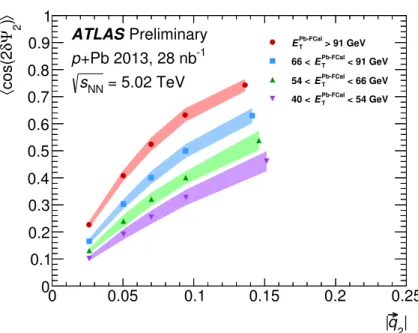
5. The EP resolution is shown in Figure 1 for the calorimeters at

η < −

2

.

5. The resolution is measured separately for both beam directions, and since they are consistent only the combined resolution is used.

4.2 Femtoscopic analysis

4.2.1 Correlation function construction

The two-particle correlation function is defined as the ratio of two-particle to single-particle momentum spectra:

C

p^a,p^b

;

k_T, φ_k

≡

dN^ab d³p^ad³p^b

! dN^a

d³p^a

! dN^b d³p^b

!,

(5)

for pairs of particles with momenta

p^a

and

p^b

. This definition has the useful feature that most single- particle efficiency, acceptance, and resolution effects cancel in the ratio. The correlation function is expressed as a function of the relative momentum

q≡ p^a−p^b

in intervals of the transverse component

k_T

of the average momentum

k≡

p^a+p^b

/

2. The azimuthal analysis is performed in intervals of

φ_k

, the azimuthal angle of

k_T

.

The events are split into classes depending on the magnitude of their flow vector, so that events are only

compared to others with similar momentum distributions. They are also sorted by the

z

position of the

2|

|q

0 0.05 0.1 0.15 0.2 0.25

〉) 2Ψδcos(2〈

0 0.1 0.2 0.3 0.4 0.5 0.6 0.7 0.8 0.9 1

> 91 GeV

Pb-FCal

ET

< 91 GeV

Pb-FCal

ET

66 <

< 66 GeV

Pb-FCal

ET

54 <

< 54 GeV

Pb-FCal

ET

40 <

Preliminary ATLAS

+Pb 2013, 28 nb-1

p

= 5.02 TeV sNN

Figure 1: The event plane (EP) resolution as a function of FCalE_Tand magnitude of the flow vector as calculated using calorimeter cells withη <−2.5. The systematic uncertainties are shown in the bands, and statistical uncertainties are too small to be visible. Only the points with the largest event activity (red) are used for the correction in this analysis, while the others are included to illustrate the dependence of the EP resolution on event activity.

primary vertex (

z_PV

), so that the background distribution is constructed with pairs of tracks originating from nearby space points. In each of these classes, the momentum distribution

A(q) ≡ dN/d³q

same

is formed by selecting pairs of particles from each event, and the combinatoric background

B(q) ≡ dN/d³q

mix

is constructed by event mixing, that is, by selecting one particle from each of two events. In the event mixing procedure, events are rotated so that their second-order event planes are aligned. Each particle in the background fulfills the same selection requirements as those used in the same-event distribution. The

A(q)

and

B(q)

histograms are combined over

z_PV

intervals in such a way that each of them sample the same

z_PV

distribution.

A correction on the same- and mixed-event distributions

A

and

B

is applied to compensate for the limited EP resolution and non-infinitesimal azimuthal bin width [30]:

A^corr

[

q,

2

(φ_k−Ψ₂)

]

= A^exp(q,

2

(φ_k−Ψ₂))+

2

ξ

A_c,2(q)

cos

2

(φ_k −Ψ₂)+ A_s,2(q)

sin

2

(φ_k−Ψ₂)

(6) where

A_c,2(q)=

1

N_bins

N_bins

X

i=1

A^expq,

2(φ

_k−Ψ₂)i

cos

2(

φ_k−Ψ₂)i

(7)

A_s,2(q)=

1

N_bins

N_bins

X

i=1

A^expq,

2(φ

_k−Ψ₂)i

sin 2(φ

_k−Ψ₂)i

(8)

and

ξ = π/N_bins

h

cos

(

2

δΨ₂)i

sin

(π/N_bins) −

1 (9)

with

N_bins =

8 being the number of azimuthal bins. The mixed-event distribution

B(q)

is also corrected with Eq. 6, and the correlation function

C(q)

is then formed by taking the ratio of the corrected same- and mixed-event relative momentum distributions

C(q)= A^corr(q) B^corr(q) .

Only the second-order harmonics are corrected in this procedure, as higher-order harmonics are not considered in this analysis.

4.2.2 Correlation function form

The Bowler-Sinyukov formalism [31, 32] is used to account for final-state corrections:

C(q)= (

1

−λ)+λK(q_inv)C_BE(q),

(10) where

K

is a correction factor for final-state Coulomb interactions as a function of Lorentz-invariant relative momentum

q_inv

parameterised by an effective source size

R_eff

, and

C_BE(q) =

1

+ F

[

S_k

]

(q)

with

F

[

Sk

]

(q)

denoting the Fourier transform of the two-particle source density function

Sk(r)

. Several factors influence the value of the parameter

λ

. Including non-identical particles decreases this parameter, as does coherent particle emission. Products of weak decays or long-lived resonances also lead to a decrease in

λ

, as they are emitted at a length scale greater than femtoscopic methods can resolve given the momentum resolution of the detector. These additional contributions to the source density are not Coulomb-corrected within the Bowler-Sinyukov formalism. When describing pion pairs of opposite charge, there is no Bose-Einstein enhancement and

C_BE=

1.

The particular choice of the correction factor

K(q_inv)

, which can modify the two-particle correlations at small relative momentum, is determined using the formalism in Ref. [33]. This uses the approximation that the Coulomb correction is effectively applied not from a point source, but over a Gaussian source density of radius

R_eff

.

The Bose-Einstein component of the three-dimensional correlation functions is fit to a function of the form

C_BE(q) =

1

+e^{− kRqk},

(11)

where

R

is a symmetric matrix in the “out-side-long” coordinate system [34–37]

R=* . . ,

R_out R_os

0

R_os R_side

0

0 0

R_long

+ / / -

.

(12)

The “out” direction is along the

k_T

of the pairs, the “side” is the other transverse direction, and the “long”

axis is along the

z

-axis, boosted to the longitudinal rest frame of the pair. The off-diagonal entry

R_ol

(which couples the “out” and “long” components) can in principle be non-zero in

z

-asymmetric collisions

like

p

+A, and in fact is observed by ATLAS to be distinct from zero in

p

+Pb collisions on the proton-

facing side of central events [16]. However, the magnitude is at largest about a factor of 50 smaller than

the diagonal radii (about 0.1 fm), and then only when analyzed as a function of pair rapidity

y^?_ππ

. In

this analysis it is fixed to zero in order to simplify the fitting procedure and focus only on the azimuthal modulation.

Exploiting symmetry arguments, the order of the particles in the pair is chosen such that

q_out

is always positive, which can be done so long as

C(−q) =C(q). As there is no off-diagonal term in R

coupling to

q_long

, the sign of

q_long

can be discarded and only

|q_long|

is considered. The sign of

q_side

cannot be similarly discarded because a non-zero

R_os

is allowed.

4.2.3 Jet fragmentation

Jet fragmentation can contribute a significant background to the correlation function, with amplitudes comparable to the femtoscopic signal itself at higher

k_T

(near 1 GeV) in peripheral events. The azimuthally- sensitive results in this analysis are measured at low

k_T

and in central events. Nevertheless, this background is constrained using the technique developed in a previous ATLAS

p

+Pb femtoscopy measurement [16].

The jet fragmentation is measured in the opposite-charge correlation functions, with the most prominent resonances removed (Section 3.4). Then, a mapping from opposite- to same-charge correlations, which is derived from a study of the fragmentation in Pythia, is used to constrain the contribution in the same-charge data. The full correlation function used in the fit is

C(q)=

1

−λ+λK(q_inv)C_BE(q)

Ω(q),

(13)

where

Ω(q)

represents the jet fragmentation contribution, and

λ

,

K(q_inv)

, and

C_BE(q)

are as defined in Section 4.2.1.

4.3 Fit procedure

Once the EP resolution correction is applied, the values in the bins of

A

and

B

are no longer Poisson- distributed. This necessitates a different choice of test statistic than that used in the previous (azimuthally- inclusive) ATLAS p+Pb femtoscopy measurement [16], which generalizes easily to allow for non-Poisson uncertainties in both

A

and

B

:

−

2 ln

L =−

2

X

binsi













A_i−B_iC(q_i)+ σ²_A

i +σ²_B

iC(q_i)²

ln

*

,

1

− A_i−B_iC(q_i) σ²_A

i +σ²_B

iC(qi)²+ -













,

(14)

where

A_i

and

B_i

are shorthand for the value in each histogram bin,

σ_Ai

and

σ_Bi

are the uncertainties in

the corresponding bin values, and the sum is taken over all bin centres

q_i

. The HBT radii are those which

minimize the above test statistic, which is taken over all histogram bins of

A

and

B

in a given

k_T

and

φ_k

interval.

4.4 Extracting Fourier components of HBT radii

The EP resolution correction induces correlations between the different azimuthal bins in

A

and

B

, since statistical fluctuations in the 2nd order Fourier coefficients are enhanced. As a result, statistical correlations in the HBT radii are induced between different azimuthal bins. The propagation of these correlations from bins of

A

and

B

through the full fitting procedure is computationally prohibitive. While enhancements to the modulation of the HBT radii are not a priori strictly linear in

ξ

, it is observed empirically that the second-order Fourier coefficients are enhanced by a factor that is consistent with the EP resolution, as in Eq. 6. To the extent that enhancements to the azimuthal modulation of the HBT radii are, like

A(q)

and

B(q)

, proportional to

ξ

(as defined in Eq. 9), imposing the same relative correlation across

φ_k

is a reasonable approximation. Thus, for the purposes of extraction of the Fourier components, the azimuthal correlations between radii are assumed to be of the same form as they are between elementary quantities like

A(q)

. A multivariate Gaussian

χ²

utilizing this non-trivial covariance matrix is then minimized to extract the zeroth- and second-order Fourier components.

The results for the HBT radii are fit to a function of the form

R_i =R_i,0

1

+

2

R_i,2

R_i,0

cos[2

(φk−Ψ₂)

]

!

,

(15)

where

i

is “out”, “side”, or “long”, while the cross-term

R_os

, which has no zeroth-order component, is fit to

R_os=

2

R_os,2

sin[2

(φ_k−Ψ₂)

]

.

(16) The allowed Fourier components for each element of the HBT matrix are discussed in Ref. [38]. In order to focus on the azimuthal modulation of the source, HBT radii and their second-order Fourier components are presented normalised by the zeroth-order Fourier component. This choice also renders the result insensitive to the non-minimum-bias nature of the data sample introduced by the HMTs. Because

R_os

has no zeroth-order component, it is instead normalized by the average of the zeroth order components of the transverse radii

R_out

and

R_side

.

5 Systematic uncertainties

The systematic uncertainties in the extracted parameter values have contributions from several sources: the jet fragmentation description, PID, the effective Coulomb correction size

R_eff

, two-particle reconstruction effects, and EP resolution. Most of these systematic uncertainties, with the exception of the EP resolution, are treated identically to those in Ref. [16].

In the previous ATLAS result, the largest source of uncertainty originated from the description of the background correlations

Ω(q)

from jet fragmentation. In this measurement, however, the high multiplicity and low

k_T

suppress the jet background. The correction and the uncertainties inherent in the mapping from opposite- to same-charge fragmentation correlations are applied the same way. The amplitude of the hard-process contribution is scaled up and down by 12.3%, which accounts for uncertainties coming from the choice of MC generator used in the study (Pythia vs. Herwig++) and from the application of

pp

MC generators in a

p

+Pb system, which was studied by comparing

pp

and

p

+Pb systems in Hijing.

An additional variation is applied on the mapping from opposite- to same-charge correlation functions by

deriving it from different rapidity ranges [16].

R_out,2/R_out,0

|~q₂|

Value Statistical Systematic Jet Frag. PID Min

q R_eff

EP Res.

0.06–0.08 -0.0364 0.0063 0.0071 0.0003 0.0034 0.0050 0.0033 0.0019 0.08–0.11 -0.0264 0.0045 0.0043 0.0006 0.0032 0.0002 0.0026 0.0010 0.11–1.0 -0.0293 0.0041 0.0038 0.0005 0.0021 0.0009 0.0029 0.0009

Table 1: Absolute statistical and systematic uncertainties of the normalized second-order Fourier component ofR_out. The values and uncertainties are displayed for three high flow intervals. All systematic uncertainties from the jet fragmentation background are combined.

The analysis is repeated at both a looser and a tighter PID selection than the nominal definition, and the variations are included as a systematic uncertainty. Because this variation involves using a subset and a super-set of the nominal data, the statistical uncertainties between the nominal and varied results are only partially correlated. This means that the uncertainties induced by this variation are conservative, since they partially overcount statistical uncertainties.

The nonzero effective size of the Coulomb correction

R_eff

should only cause a typical point-to-point change in the correlation function of a few percent, even with a value up to several femtometers, since the Bohr radius of pion pairs is nearly 400 fm. However, since this parameter changes the width in

|q|

over which the Coulomb correction is applied, varying this parameter can affect the source radii measurably.

The effective size is assumed to scale with the size of the source itself, so a scaling constant

R_eff/R_inv

is chosen, where

R_inv

is extracted from the one-dimensional correlation function constructed from

q_inv

. The nominal value of

R_eff/R_inv

is taken to be equal to 1 and the associated systematic uncertainty is evaluated by varying this between 1/2 and 2.

Single-particle correction factors for track reconstruction efficiency cancel in the ratio

A(q)/B(q). How-

ever, two-particle effects in the track reconstruction can affect the correlation function at small relative momentum. Single- and multi-track reconstruction effects are both studied with the fully simulated Hijing sample. The generator-level and reconstructed correlation functions are compared, and a deficit in

|q|

below approximately 50 MeV is observed while at larger

|q|

the effect is absent within statistical uncertainties. A minimum

|q|

cutoff is applied in the fits to minimize the impact of these detector effects.

The sensitivity of the results to this cutoff is evaluated by symmetrising the effect of the variation from

|q|^min=

25 to 50 MeV.

Uncertainty in the second-order EP resolution is propagated to the results through the event plane resolution correction. There are two contributions to the

Ψ₂

resolution uncertainty, both of which are evaluated by changes to the two alternate subevents used in the three-subevent method of evaluating

h

cos

(

2

δΨ₂)i

. For one variation, the rapidity windows of the alternate subsdetectors are shifted away from the nominal sub-detector by

∆η =

0

.

5. For the other variation, which has a smaller effect, tracks weighted by their

p_T

are used instead of calorimeter cells.

Tables 1–3 show the uncertainties contributing to the relative modulation of

R_out

,

R_side

, and

R_long

.

R_side,2/R_side,0

|~q₂|

Value Statistical Systematic Jet Frag. PID Min

q R_eff

EP Res.

0.06–0.08 0.0086 0.0061 0.0056 0.0006 0.0043 0.0034 0.0003 0.0005 0.08–0.11 0.0116 0.0044 0.0016 0.0008 0.0011 0.0004 0.0005 0.0005 0.11–1.0 0.0096 0.0040 0.0024 0.0005 0.0022 0.0009 0.0004 0.0003

Table 2: Absolute statistical and systematic uncertainties of the normalized second-order Fourier component of R_side. The values and uncertainties are displayed for three high flow intervals. All systematic uncertainties from the jet fragmentation background are combined.

R_long,2/R_long,0

|~q₂|

Value Statistical Systematic Jet Frag. PID Min

q R_eff

EP Res.

0.06–0.08 0.0077 0.0061 0.0050 0.0003 0.0030 0.0039 0.0002 0.0004 0.08–0.11 0.0183 0.0044 0.0021 0.0006 0.0016 0.0010 0.0002 0.0007 0.11–1.0 0.0145 0.0040 0.0019 0.0002 0.0004 0.0018 0.0002 0.0004

Table 3: Absolute statistical and systematic uncertainties of the normalized second-order Fourier component of R_long. The values and uncertainties are displayed for three high flow intervals. All systematic uncertainties from the jet fragmentation background are combined.

6 Results

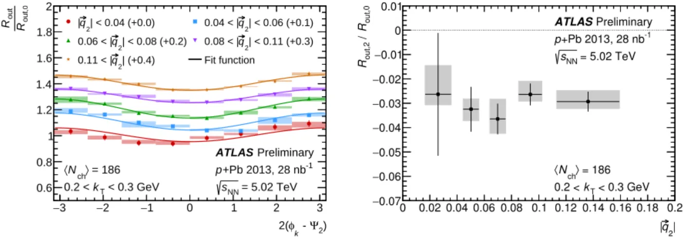
The relative modulation of the source radii is shown in the left panels of Figures 2–4 for

R_out

,

R_side

, and

R_long

, respectively. A

k_T

interval from 0.2 to 0.3 GeVis shown, as this momentum is sufficiently low to represent the late stages of the evolution. The transverse radii,

R_out

and

R_side

, show significant modulation in the orientation compatible with the initial elliptic orientation predicted by hydrodynamics.

R_out

, presented in Figure 2, has a stronger modulation than the other two radii.

2) Ψ

k - φ 2(

−3 −2 −1 0 1 2 3

,0outR

outR

0.6 0.8 1 1.2 1.4 1.6 1.8 2

| < 0.04 (+0.0) q2

| | < 0.06 (+0.1)

q2

0.04 < |

| < 0.08 (+0.2) q2

0.06 < | | < 0.11 (+0.3)

q2

0.08 < |

| (+0.4) q2

0.11 < | Fit function

< 0.3 GeV kT

0.2 <

= 186

ch〉

〈N

Preliminary ATLAS

+Pb 2013, 28 nb-1

p

= 5.02 TeV sNN

2|

|q 0 0.02 0.04 0.06 0.08 0.1 0.12 0.14 0.16 0.18 0.2

,0outR / ,2outR

0.07

− 0.06

− 0.05

− 0.04

− 0.03

− 0.02

− 0.01

− 0 0.01

Preliminary ATLAS

+Pb 2013, 28 nb-1

p

= 5.02 TeV sNN

< 0.3 GeV kT

0.2 <

= 186

ch〉 N

〈

Figure 2: The outwards HBT radius R_out as a function of angular distance from the second-order event plane 2(φ_k−Ψ₂)(left) and the second-order Fourier coefficient (right) as a function of flow vector magnitude|~q₂|, both of which are normalized by the zeroth-order Fourier coefficient. The vertical bars indicate statistical uncertainty while shaded boxes indicate systematic uncertainties added in quadrature. The points in different intervals of|~q₂| are offset in the left plot for visibility, as indicated in the legend. Each set of points is fit to a function of the form R_out=R_out,0+2R_out,2cos

2(φ_k−Ψ₂)

. The width of the boxes in the right plot indicates the standard deviation of

|~q₂|in each interval.hN_chiis shown to provide an indication of the event activity of the sample.

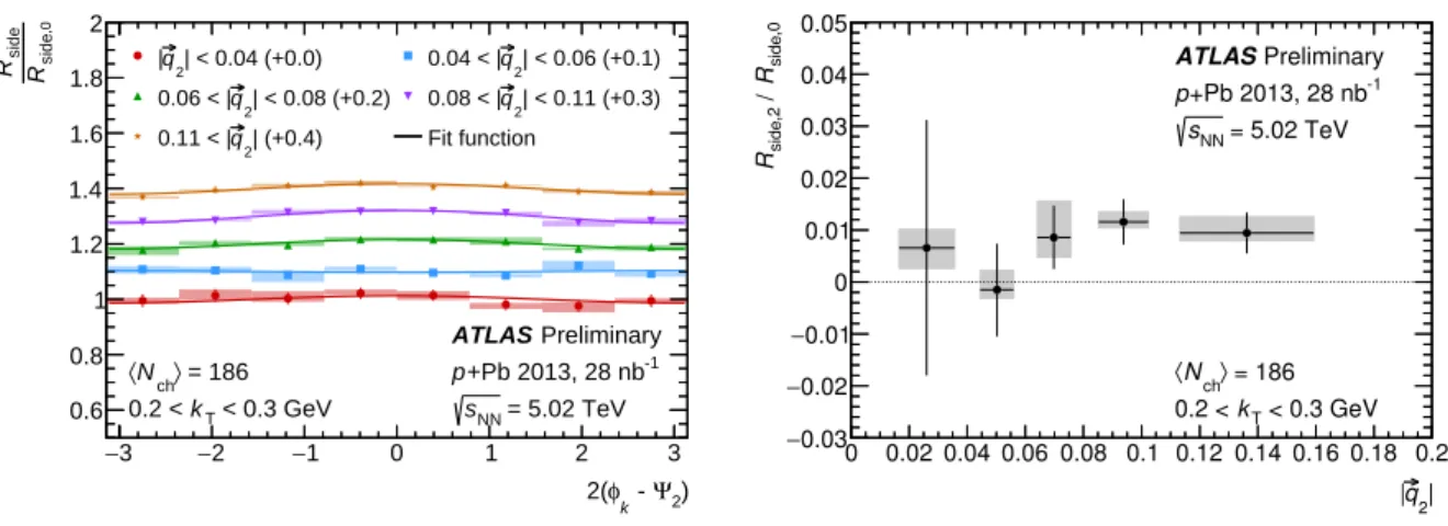
The sideways radius

R_side

, shown in Figure 3, gives a cleaner picture of the geometrical modulation.

Since

R_side

indicates a length perpendicular to the pair’s transverse momentum, the fact that it is larger in-plane than out-of-plane indicates that the source is spatially extended out-of-plane at freeze-out. As the modulation of

R_out

is in the other direction, this is consistent with an elliptical transverse density with its minor axis aligned with the EP, as predicted by hydrodynamics.

2) Ψ

k - φ 2(

−3 −2 −1 0 1 2 3

,0sideR

sideR

0.6 0.8 1 1.2 1.4 1.6 1.8 2

| < 0.04 (+0.0) q2

| | < 0.06 (+0.1)

q2

0.04 < |

| < 0.08 (+0.2) q2

0.06 < | | < 0.11 (+0.3)

q2

0.08 < |

| (+0.4) q2

0.11 < | Fit function

< 0.3 GeV kT

0.2 <

= 186

ch〉

〈N

Preliminary ATLAS

+Pb 2013, 28 nb-1

p

= 5.02 TeV sNN

2|

|q 0 0.02 0.04 0.06 0.08 0.1 0.12 0.14 0.16 0.18 0.2

,0sideR / ,2sideR

0.03

− 0.02

− 0.01

− 0 0.01 0.02 0.03 0.04 0.05

Preliminary ATLAS

+Pb 2013, 28 nb-1

p

= 5.02 TeV sNN

< 0.3 GeV kT

0.2 <

= 186

ch〉 N

〈

Figure 3: The sideways HBT radius R_side as a function of angular distance from the second-order event plane 2(φ_k−Ψ₂)(left) and the second-order Fourier coefficient (right) as a function of flow vector magnitude|~q₂|, both of which are normalized by the zeroth-order Fourier coefficient. The vertical bars indicate statistical uncertainty while shaded boxes indicate systematic uncertainties added in quadrature. The points in different intervals of|~q₂| are offset in the left plot for visibility, as indicated in the legend. Each set of points is fit to a function of the form R_side=R_side,0+2R_side,2cos

2(φ_k−Ψ₂)

. The width of the boxes in the right plot indicates the standard deviation of|~q₂|in each interval.hN_chiis shown to provide an indication of the event activity of the sample.

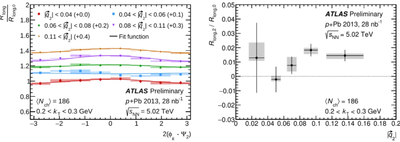
The longitudinal radius

R_long

is shown in Figure 4, where it displays comparable modulation in sign and magnitude to

R_side

. This could suggest that the source experiences greater longitudinal expansion in-plane than out-of-plane.

The cross term coupling the

R_out

and

R_side

terms,

R_os

, is presented in Figure 5. Since it has no zeroth Fourier component, it is normalized by the mean of

R_out,0

and

R_side,0

. The sign of the modulation is also consistent with that observed in A-A collisions [17–19].

Some additional combinations of the HBT radii are also presented along with their azimuthal modulation.

Figure 6 shows the ratio

R_out/R_side

, which is understood to be a measurement of the lifetime, since in hydrodynamic models

R_out

is sensitive to the lifetime and

R_side

is not.

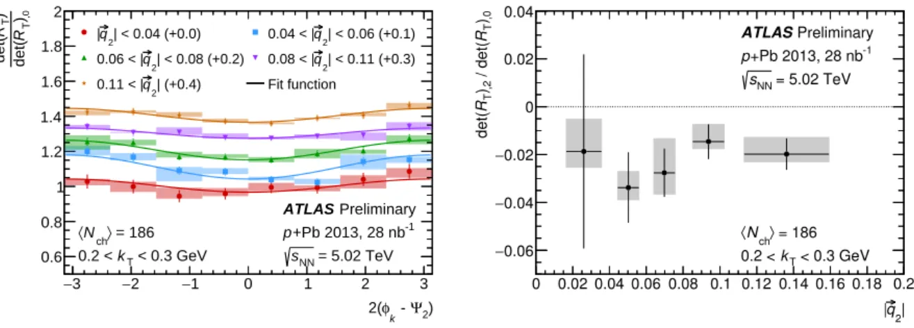
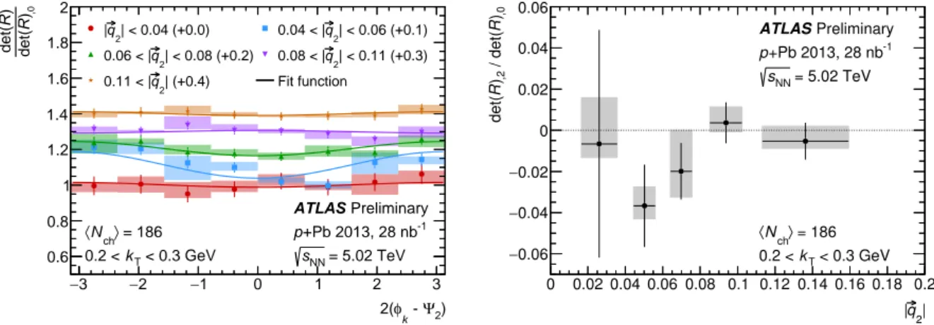
Figures 7–8 show the determinants of the transverse projection of the HBT matrix [det

(R_T)

] and of the full 3D matrix [det

(R)

]. The transverse determinant displays some in-plane suppression and out-of-plane enhancement, while the 3D volume element shows no modulation within the uncertainties.

In each of the results shown in this section, the modulation at low

|~q₂|

cannot be distinguished from zero

within uncertainties. Hydrodynamics does not predict elliptical spatial anisotropies in events with low flow,

and the vanishing event plane resolution makes the measurement difficult in that limit, which is reflected

in the large statistical uncertainties in the second-order components of the radii. The conclusions from

these results should be drawn primarily from the trend of the relative modulation in events characterised

by higher values of

|~q₂|

, where the low EP resolution does not deteriorate the measurement.

2) Ψ

k - φ 2(

−3 −2 −1 0 1 2 3

,0longR

longR

0.6 0.8 1 1.2 1.4 1.6 1.8 2

| < 0.04 (+0.0) q2

| | < 0.06 (+0.1)

q2

0.04 < |

| < 0.08 (+0.2) q2

0.06 < | | < 0.11 (+0.3)

q2

0.08 < |

| (+0.4) q2

0.11 < | Fit function

< 0.3 GeV kT

0.2 <

= 186

ch〉

〈N

Preliminary ATLAS

+Pb 2013, 28 nb-1

p

= 5.02 TeV sNN

2|

|q 0 0.02 0.04 0.06 0.08 0.1 0.12 0.14 0.16 0.18 0.2

,0longR / ,2longR

0.03

− 0.02

− 0.01

− 0 0.01 0.02 0.03 0.04 0.05

Preliminary ATLAS

+Pb 2013, 28 nb-1

p

= 5.02 TeV sNN

< 0.3 GeV kT

0.2 <

= 186

ch〉 N

〈

Figure 4: The longitudinal HBT radius R_long as a function of angular distance from the second-order event plane 2(φ_k−Ψ₂)(left) and the second-order Fourier coefficient (right) as a function of flow vector magnitude|~q₂|, both of which are normalized by the zeroth-order Fourier coefficient. The vertical bars indicate statistical uncertainty while shaded boxes indicate systematic uncertainties added in quadrature. The points in different intervals of|~q₂| are offset in the left plot for visibility, as indicated in the legend. Each set of points is fit to a function of the form R_long =R_long,0+2R_long,2cos

2(φ_k−Ψ₂)

. The width of the boxes in the right plot indicates the standard deviation of|~q₂|in each interval.hN_chiis shown to provide an indication of the event activity of the sample.

2) Ψ

k - φ 2(

−3 −2 −1 0 1 2 3

,0sideR + ,0outR

osR2

−0.4

−0.2 0 0.2 0.4 0.6 0.8 1

| < 0.04 (+0.0) q2

| | < 0.06 (+0.1)

q2

0.04 < |

| < 0.08 (+0.2) q2

0.06 < | | < 0.11 (+0.3)

q2

0.08 < |

| (+0.4) q2

0.11 < | Fit function

< 0.3 GeV kT

0.2 <

= 186

ch〉

〈N

Preliminary ATLAS

+Pb 2013, 28 nb-1

p

= 5.02 TeV sNN

2|

|q 0 0.02 0.04 0.06 0.08 0.1 0.12 0.14 0.16 0.18 0.2

,0sideR + ,0outR / ,2osR2

0.01

− 0.005

− 0 0.005 0.01 0.015 0.02 0.025 0.03 0.035 0.04

< 0.3 GeV kT

0.2 <

= 186

ch〉 N

〈

= 5.02 TeV sNN

+Pb 2013, 28 nb-1

p

Preliminary ATLAS

Figure 5: The out-side cross-termR_osas a function of angular distance from the second-order event plane 2(φ_k−Ψ₂) (left), along with the second Fourier sine coefficient (right), as a function of flow vector magnitude|~q₂|. The vertical bars indicate statistical uncertainty while shaded boxes indicate systematic uncertainties added in quadrature. It is normalized by the mean of the zeroth-order Fourier coefficients of the transverse HBT radiiR_outand R_side. The points in different intervals of|~q₂| are offset in the left plot for visibility, as indicated in the legend. Each set of points is fit to a function of the formR_os=2R_os,2sin

2(φ_k−Ψ₂)

. The width of the boxes in the right plot indicates the standard deviation of|~q₂|in each interval. hN_chiis shown to provide an indication of the event activity of the sample.

2) Ψ

k - φ 2(

−3 −2 −1 0 1 2 3

sideR

outR

0.4 0.6 0.8 1 1.2 1.4 1.6 1.8

| < 0.04 (+0.0) q2

| | < 0.06 (+0.1)

q2

0.04 < |

| < 0.08 (+0.2) q2

0.06 < | | < 0.11 (+0.3)

q2

0.08 < |

| (+0.4) q2

0.11 < | Fit function

< 0.3 GeV kT

0.2 <

= 186

ch〉

〈N

Preliminary ATLAS

+Pb 2013, 28 nb-1

p

= 5.02 TeV sNN

2|

|q 0 0.02 0.04 0.06 0.08 0.1 0.12 0.14 0.16 0.18 0.2

,0 sideR

outR / ,2 sideR

outR

0.07

− 0.06

− 0.05

− 0.04

− 0.03

− 0.02

− 0.01

− 0 0.01

Preliminary ATLAS

+Pb 2013, 28 nb-1

p

= 5.02 TeV sNN

< 0.3 GeV kT

0.2 <

= 186

ch〉 N

〈

Figure 6: The ratio R_out/R_side as a function of angular distance from the second-order event plane 2(φ_k −Ψ₂) (left), along with the normalized second-order Fourier coefficient (right), as a function of flow vector magnitude

|~q₂|. The vertical bars indicate statistical uncertainty while shaded boxes indicate systematic uncertainties added in quadrature. The points in different intervals of|~q₂|are offset in the left plot for visibility, as indicated in the legend.

Each set of points is fit to a function of the formR_out/R_side=(R_out/R_side)_,0+2(R_out/R_side)_,2cos

2(φ_k−Ψ₂) . The width of the boxes in the right plot indicates the standard deviation of|~q₂|in each interval. hN_chiis shown to provide an indication of the event activity of the sample.

2) Ψ

k - φ 2(

−3 −2 −1 0 1 2 3

,0)TRdet()TRdet(

0.6 0.8 1 1.2 1.4 1.6 1.8 2

| < 0.04 (+0.0) q2

| | < 0.06 (+0.1)

q2

0.04 < |

| < 0.08 (+0.2) q2

0.06 < | | < 0.11 (+0.3)

q2

0.08 < |

| (+0.4) q2

0.11 < | Fit function

< 0.3 GeV kT

0.2 <

= 186

ch〉

〈N

Preliminary ATLAS

+Pb 2013, 28 nb-1

p

= 5.02 TeV sNN

2|

|q 0 0.02 0.04 0.06 0.08 0.1 0.12 0.14 0.16 0.18 0.2

,0)TR / det(,2)TRdet(

0.06

− 0.04

− 0.02

− 0 0.02 0.04

Preliminary ATLAS

+Pb 2013, 28 nb-1

p

= 5.02 TeV sNN

< 0.3 GeV kT

0.2 <

= 186

ch〉 N

〈

Figure 7: The transverse area element of the HBT matrix det(R_T) as a function of angular distance from the second-order event plane 2(φ_k −Ψ₂) (left) and the second-order Fourier coefficient (right) as a function of flow vector magnitude|~q₂|, both normalized by the zeroth-order Fourier coefficient. The vertical bars indicate statistical uncertainty while shaded boxes indicate systematic uncertainties added in quadrature. The points in different intervals of|~q₂|are offset in the left plot for visibility, as indicated in the legend. Each set of points is fit to a function of the form det(R_T) =det(R_T)_,0+2det(R_T)_,2cos

2(φ_k−Ψ₂)

. The width of the boxes in the right plot indicates the standard deviation of|~q₂|in each interval. hN_chiis shown to provide an indication of the event activity of the sample.