ATLAS-CONF-2019-013 11May2019
ATLAS CONF Note
ATLAS-CONF-2019-013
10th May 2019
Searches for lepton-flavour-violating decays of the Higgs boson in √
s = 13 TeV p p collisions with the ATLAS detector
The ATLAS Collaboration
This note presents direct searches for lepton flavour violation in Higgs boson decays,
H→eτand
H → µτ, performed with the ATLAS detector at the LHC. The searches are based on a data sample of
ppcollisions at a centre-of-mass energy
√s =
13 TeV, corresponding to an integrated luminosity of 36
.1 fb
−1. No significant excesses over the SM predictions are observed and upper limits on the lepton-flavour-violating branching ratios are set. The observed (median expected) 95% confidence level upper limits are 0
.47% (0
.34
+0−0..1310%) and 0
.28% (0
.37
+0−0..1410%) for
H→eτand
H→ µτ, respectively.
© 2019 CERN for the benefit of the ATLAS Collaboration.
Reproduction of this article or parts of it is allowed as specified in the CC-BY-4.0 license.
1 Introduction
The search for physics beyond the Standard Model (SM) is one of the main goals of the Large Hadron Collider (LHC) programme at CERN. A possible sign of such physics is lepton flavour violation (LFV) in decays of the Higgs boson [1, 2]. Many beyond-SM theories predict LFV decays of the Higgs boson, such as extensions of the Higgs sector or warped extra dimension models [3–6].
In this note, searches for LFV decays of the Higgs boson,
H →eτand
H → µτ, at the LHC with the ATLAS experiment are presented. Studies are based on
ppcollision data recorded in 2015-2016 at the centre-of-mass energy
√s =
13 TeV. The dataset corresponds to an integrated luminosity of 36
.1 fb
−1. Previous ATLAS searches [7, 8] placed an upper limit of 1.04% (1.43%) on the
H → eτ(
H → µτ) branching ratio (
B) with a 95% confidence level (CL) using Run 1 data collected at
√s =
8 TeV (corresponding to an integrated luminosity of 20
.3 fb
−1). The CMS collaboration recently provided 95%
CL upper limits on these branching ratios of 0.61% and 0.25%, respectively, using data collected at
√s=
13 TeV, with an integrated luminosity of 35
.9 fb
−1[9].
The searches presented here involve both leptonic (
τ→`0νν¯
1) and hadronic (τ→hadrons
+ν) decays of
τ-leptons, denoted
τ`0and
τhadrespectively. Only pairs of different-flavour leptons are considered in the di-lepton final states
`τ`0. Two channels are considered for each of the two searches:
eτµand
eτhadfor the
H →eτsearch,
µτeand
µτhadfor the
H→ µτsearch. The analysis is designed such that any potential LFV signal overlap between the
H→eτand
H→µτsearches is negligible. Many methods are re-used from the measurement of the Higgs boson cross-section in the
H→ττfinal state [10].
2 ATLAS detector
The ATLAS detector2 is described in Refs. [11, 12]. It consists of an inner tracking detector covering the range
|η| <2
.5, surrounded by a superconducting solenoid providing a 2 T axial magnetic field, and high-granularity electromagnetic (
|η| <3
.2) and hadronic calorimeters (
|η| <4
.9). It is completed by the muon spectrometer (MS) covering the range
|η|<2
.7 with a toroidal field in the outer part and including fast trigger chambers (
|η| <2
.4).
3 Simulation samples
Samples of Monte Carlo simulated events (MC) are used to optimize the event selection, and to model signal and several of the background processes. The samples are produced with the ATLAS simulation infrastructure [13] using the full detector simulation performed by the Geant4 [14] toolkit. The Higgs boson mass is set to
mH =125 GeV [15]. The four leading Higgs boson production mechanisms are considered – the gluon-gluon fusion (ggF), vector boson fusion (VBF) and two associated production modes (
W H,
Z H), while the others have negligible contributions and have been ignored. The cross-sections of all Higgs boson production processes are fixed to the SM predictions [16]. The LFV Higgs boson
1Unless explicitly mentioned otherwise, leptons (denoted by`or`0) refer to electrons or muons.
2ATLAS uses a right-handed coordinate system with its origin at the nominal interaction point in the centre of the detector and thez-axis along the beam pipe. The azimuthal angleφruns around the beam pipe, the pseudorapidity is defined in terms of the polar angleθasη≡ −ln tan(θ/2). The distance in theη−φspace is defined as∆R≡p
(∆η)2+(∆φ)2.
decays as well as the
H→ττand
H→WWbackground decays are modelled with Pythia 8 [17]. Other background processes involve electro-weak production of
W/Zbosons via VBF, Drell-Yan production of
W/Zin association with jet(s) as well as di-boson, single-top-quark and
t¯tproduction. The MCs used for the SM
H→ττcross-section measurement [10] are also employed here for all background components.
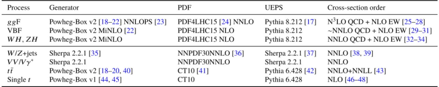
The generators and parton showers used to simulate different processes are summarized in Table 1.
Table 1: Generators used to describe the signal and background processes, parton distribution function (PDF) sets for the hard process, and models used for parton showering, hadronization and underlying event (UEPS). The orders of the total cross-sections used to normalize the events are also given. More details are given in Ref. [10].
Process Generator PDF UEPS Cross-section order
ggF Powheg-Box v2 [18–22] NNLOPS [23] PDF4LHC15 [24] NNLO Pythia 8.212 [17] N3LO QCD + NLO EW [25–28]
VBF Powheg-Box v2 MiNLO [22] PDF4LHC15 NLO Pythia 8.212 ∼NNLO QCD + NLO EW [29–31]
W H,Z H Powheg-Box v2 MiNLO PDF4LHC15 NLO Pythia 8.212 NNLO QCD + NLO EW [32–34]
W/Z+jets Sherpa 2.2.1 [35] NNPDF30NNLO [36] Sherpa 2.2.1 [37] NNLO [38,39]
VV/Vγ∗ Sherpa 2.2.1 NNPDF30NNLO Sherpa 2.2.1 NNLO
t¯t Powheg-Box v2 [18–20,40] CT10 [41] Pythia 6.428 [42] NNLO+NNLL [43]
Singlet Powheg-Box v1 [44,45] CT10 Pythia 6.428 NLO [46–48]
4 Object reconstruction
The correct identification of
H →`τevents requires reconstruction of most physics objects (electrons, muons, and jets, including those initiated by hadronic decays of
τ-leptons) and the missing transverse energy
EmissT
.
Electrons are reconstructed by matching tracks from the inner detector to clustered energy deposits in the electromagnetic calorimeter [49]. A loose likelihood-based identification [50],
pT >15 GeV and fiducial volume requirements (
|η| <2
.47, excluding the transition region between the barrel and the endcap calorimeters 1
.37
< |η| <1
.52) are applied. Medium identification and gradient isolation [50] criteria are required for the baseline electron selection.
Muons are identified by tracks reconstructed in the inner detector and matched to tracks from the MS.
Loose identification [51],
pT >10 GeV and
|η| <2
.5 are applied. Medium identification and gradient isolation [51] are required for the baseline muon selection.
Jets are reconstructed using the anti-
ktalgorithm [52] with a radius parameter
R=0
.4 applied to topological clusters of calorimeter cells [53]. Only jets with
pT >20 GeV and
|η| <4
.5 are considered. Jets from other
ppinteractions in the same and neighbouring bunch crossings (pile-up) are suppressed using jet vertex tagger (JVT) algorithms [54, 55]. Jets containing
b-hadrons (
b-jets) are identified by the MV2c20 algorithm [56, 57] in the central region (
|η| <2
.4). A working point corresponding to 85% average efficiency determined for
b-jets from
tt¯ MC is chosen.
The reconstruction of the object formed by the visible products of the
τhaddecay (
τhad-vis) begins from the energy deposits in the calorimeter, processed by the anti-
ktjet algorithm with a radius parameter
R=0
.4.
Information from the inner detector tracks associated to the energy deposits in the calorimeter is incorporated in the reconstruction. Only
τhad-viscandidates with
pT >20 GeV and
|η| <2
.5 are considered.3 One or three associated charged tracks and an absolute charge
|q| =1 are required. An identification algorithm [58,
3The transition region inηis excluded, similarly to electrons.
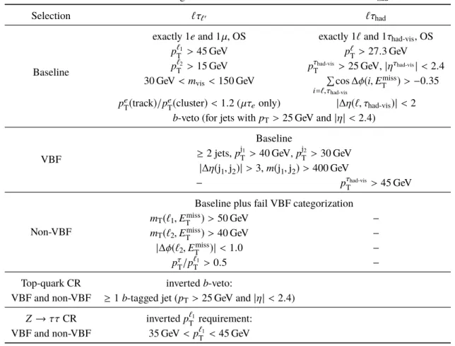
Table 2: Baseline event selection and further categorization for the`τ`0and`τhadchannels. The same criteria are also used for the control region (CR) definitions in the`τ`0channel (see Section6), nevertheless one requirement of the baseline selection is inverted to achieve orthogonal event selection. There is no CR in the`τhadchannel.
Selection `τ`0 `τhad
Baseline
exactly 1eand 1µ, OS exactly 1`and 1τhad-vis, OS p`1
T >45 GeV p`
T>27.3 GeV p`2
T >15 GeV pτhad-vis
T >25 GeV,|ητhad-vis|<2.4 30 GeV<mvis<150 GeV Í
i=`,τhad-vis
cos∆φ(i,Emiss
T )>−0.35 pe
T(track)/pe
T(cluster)<1.2 (µτeonly) |∆η(`, τhad-vis)|<2 b-veto (for jets withpT>25 GeV and|η|<2.4)
VBF
Baseline
≥2 jets,pj1
T >40 GeV,pj2
T >30 GeV
|∆η(j1,j2)|>3,m(j1,j2)>400 GeV
− pτhad-vis
T >45 GeV
Non-VBF
Baseline plus fail VBF categorization mT(`1,Emiss
T )>50 GeV −
mT(`2,Emiss
T )>40 GeV −
|∆φ(`2,Emiss
T )|<1.0 −
pτ
T/p`1
T >0.5 −
Top-quark CR invertedb-veto:
VBF and non-VBF ≥1b-tagged jet (pT>25 GeV and|η| <2.4)
Z →ττCR invertedp`1
T requirement:
VBF and non-VBF 35 GeV<p`1
T <45 GeV
59] based on Boosted Decision Trees (BDT) [60–62] is used to reject
τhad-viscandidates initiated by quarks or gluons. Unless otherwise indicated, a tight identification (ID) working point of the
τhad-visis required, corresponding to an efficiency of 60% (45%) for 1-prong (3-prong) candidates. The
τhad-viscandidates with one track overlapping with an electron candidate with high ID score, as determined by a multivariate (MVA) approach, are rejected. Leptonic
τ-decays are reconstructed as electrons or muons.
Single lepton triggers with
pTthresholds between 21 and 27 GeV, depending on the trigger type and data-taking period, and variable isolation requirements are used for both the
`τ`0and
`τhadfinal states [63, 64].
5 Event selection and categorization
Events selected in the
`τ`0channel contain exactly one electron and one muon of opposite-sign (OS)
charges. Similarly in the
`τhadchannel, a lepton and a
τhad-visof opposite charge are required, and events
with more than one lepton are rejected. The selection criteria are summarized in Table 2 for the analysis
categories as well as the control regions (CR) which are described in Section 6.
In the
`τ`0channel,
`1and
`2denote the leading and subleading lepton in
pT, respectively. A requirement on the di-lepton invariant mass, equal to the invariant mass of the lepton and the visible
τ-decay products,
mvis, reduces backgrounds with top-quarks, and the criterion applied on the track-to-cluster
pTratio of the electron reduces the
Z → µµbackground where a muon deposits a large amount of energy in the electromagnetic calorimeter and is mis-identified as an electron in the
µτechannel. The contribution from the
H→ττdecay is reduced by the asymmetric
pTselection criteria on the two leptons.
In the
`τhadchannel, the criterion based on the azimuthal separations of lepton–
EmissT
and
τhad-vis–
EmissT
,
Íi=`,τhad-vis
cos
∆φ(i,EmissT )
, reduces the
W+jets background whereas the|∆η(`, τhad-vis)|requirement reduces sources of backgrounds with mis-identified
τhad-viscandidates.
For both channels, a
b-veto requirement reduces the single-top-quark and
tt¯ backgrounds. Events are further categorized into VBF (with a focus on the VBF production of the Higgs boson) and non-VBF categories. The VBF selection is based on the kinematics of two jets with the highest
pT, where j
1and j
2denote the leading and subleading jet in
pT, respectively. The variables
m(j
1,j
2)and
∆η(j
1,j
2)stand for the invariant mass and
ηseparation of these two jets. The non-VBF category contains events failing the VBF selection. Additional selection criteria in
`τ`0, as described in Table 2, are applied to further reject background events in this category, in which
mTstands for the transverse mass4 of the two objects listed in parentheses, and
pτT
represents the magnitude of the vector sum of
p`2T
and
EmissT
. The
pτT/p`1
T
requirement reduces the background arising from jets mis-identified as leptons. The VBF and non-VBF categories in each of the
`τ`0and
`τhadchannels give rise to four signal regions in each search.
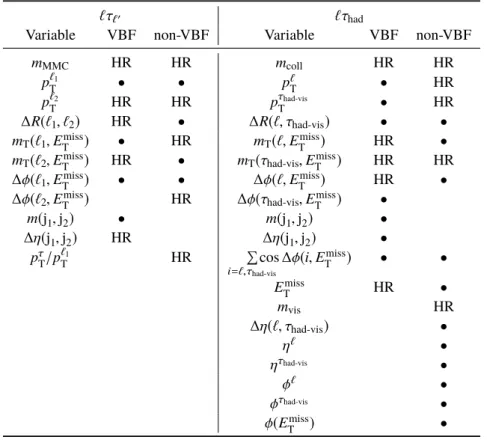
The analysis exploits BDT algorithms to enhance the signal separation from the background in the individual searches, channels and categories. First, the components of the four-momenta of the analysis objects as well as derived event variables (e.g. invariant masses and angular separations) are the input variables of the BDT discriminant. This list of variables is then optimized, removing those with the lowest discriminating power according to Refs. [65, 66]. The final list of variables is presented in Table 3 for each channel and category. The invariant mass of the Higgs boson reconstructed under the
H →`τdecay hypothesis exhibits the highest signal-to-background separation power and it helps to distinguish LFV signal from
H→ττand
H→WWbackgrounds. The invariant mass is reconstructed with the MMC algorithm [67],
mMMC, for the
`τ`0channel and under the collinear approximation [67],
mcoll, for the
`τhadchannel. The analysis CRs have been used to validate the agreement between data and simulated distributions of the BDT score and input variables, as well as their correlations.
4The transverse mass of two objects is defined asmT=p
2pT1pT2(1−cos∆φ), wherepTiare the individual transverse momenta and∆φis the angle between the two objects in the azimuthal plane.
Table 3: BDT input variables used in the analysis. For each channel and category, used input variables are marked with HR (indicating the five variables with the highest rank) or a bullet. Analogous variables between the two channels are listed on the same line.
`τ`0 `τhad
Variable VBF non-VBF Variable VBF non-VBF
mMMC HR HR mcoll HR HR
p`1
T • • p`
T • HR
p`2
T HR HR pτhad-vis
T • HR
∆R(`1, `2) HR • ∆R(`, τhad-vis) • • mT(`1,Emiss
T ) • HR mT(`,Emiss
T ) HR •
mT(`2,Emiss
T ) HR • mT(τhad-vis,Emiss
T ) HR HR
∆φ(`1,Emiss
T ) • • ∆φ(`,Emiss
T ) HR •
∆φ(`2,Emiss
T ) HR ∆φ(τhad-vis,Emiss
T ) •
m(j1,j2) • m(j1,j2) •
∆η(j1,j2) HR ∆η(j1,j2) • pτ
T/p`1
T HR Í
i=`,τhad-vis
cos∆φ(i,Emiss
T ) • •
Emiss
T HR •
mvis HR
∆η(`, τhad-vis) •
η` •
ητhad-vis •
φ` •
φτhad-vis •
φ(Emiss
T ) •
6 Background modelling
The most significant backgrounds to a potential LFV signal are the
Z →ττand (single- or pair-produced) top-quark processes, especially in the
`τ`0channel, as well as backgrounds from mis-identified objects, which are estimated using data-driven techniques. The relative contribution from mis-identified objects to the total background yield is 5–25% in the
`τ`0channel and 25–45% in the
`τhadchannel, depending on the search and the analysis category. The shapes of the
Z →ττ, single-top-quark and
t¯tprocesses are modelled by simulation in both the
`τ`0and
`τhaddecay channels. In the
`τ`0channel, the relative contributions of
Z →ττand top-quark production processes are 20–35% and 20–55%, respectively; the top-quark background dominates in the VBF category. In the
`τhadchannel, the top-quark background fraction is 1–10%, while the
Z → ττprocess contributes to 45–55% of the total background. The individual contributions are listed in Tables 4 and 5. Smaller background components are also modelled by simulation and are grouped together:
Z →µµ, di-boson production,
H→ττand
H→WW.
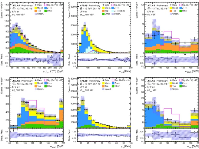
Good modelling of the background is demonstrated in Fig. 1 for a selection of important BDT input
variables. More details on the background estimation techniques are given below.
) [GeV]
miss
ET 1 , (l mT
60 80 100 120 140 160 180 200 220 240
Data / Pred.
0.5 0.75 1 1.25 1.5
Events / 10 GeV
0 200 400 600 800 1000 1200 1400 1600
1800 ATLASPreliminary = 13 TeV, 36.1 fb-1
s LFV eτ
non-VBF τµ
e
Data Sig. (B=1%)×10 Mis-id. Z→ττ
Top Other
Uncert.
[GeV]
mcoll
50 100 150 200 250 300
Data / Pred.
0.5 0.75 1 1.25 1.5
Events / 10 GeV
0 10000 20000 30000 40000
50000 ATLASPreliminary = 13 TeV, 36.1 fb-1
s LFV eτ
non-VBF τhad
e
Data Sig. (B=1%)×10 Mis-id. Z→ττ Top Z→ee (d.d.) Other Uncert.
[GeV]
mMMC
60 80 100 120 140 160 180 200
Data / Pred.
0.5 0.75 1 1.25 1.5
Events / 10 GeV
0 20 40 60 80
100 ATLASPreliminary = 13 TeV, 36.1 fb-1
s LFV eτ
µ VBF eτ
Data Sig. (B=1%)×10 Mis-id. Z→ττ
Top Other
Uncert.
[GeV]
mMMC
60 80 100 120 140 160 180 200
Data / Pred.
0.5 0.75 1 1.25 1.5
Events / 10 GeV
0 200 400 600 800 1000
1200 ATLASPreliminary = 13 TeV, 36.1 fb-1
s τ LFV µ
non-VBF τe
µ
Data Sig. (B=1%)×10 Mis-id. Z→ττ
Top Other
Uncert.
[GeV]
l
pT
30 40 50 60 70 80 90 100
Data / Pred.
0.5 0.75 1 1.25 1.5
Events / 5 GeV
0 10000 20000 30000 40000 50000 60000 70000 80000
ATLASPreliminary = 13 TeV, 36.1 fb-1
s τ LFV µ
non-VBF τhad
µ
Data Sig. (B=1%)×10 Mis-id. Z→ττ
Top Other
Uncert.
[GeV]
mcoll
60 80 100 120 140 160 180 200
Data / Pred.
0.5 0.75 1 1.25 1.5
Events / 10 GeV
0 20 40 60 80 100 120 140
160 ATLASPreliminary = 13 TeV, 36.1 fb-1
s τ LFV µ
had VBF τ µ
Data Sig. (B=1%)×10 Mis-id. Z→ττ
Top Other
Uncert.
Figure 1: Pre-fit distributions of representative kinematic quantities for different searches, channels and categories.
Top row: transverse massmT(`1,Emiss
T )(eτµnon-VBF), collinear massmcoll(eτhadnon-VBF) andmMMC(eτµVBF).
Bottom row: mMMC(µτenon-VBF), muonpT(µτhadnon-VBF) andmcoll(µτhadVBF). Entries with values that would exceed thex-axis range are included in the last bin of each distribution. The size of the combined statistical, experimental and theoretical uncertainties in the background is indicated by the hatched bands. TheH → eτ (H→ µτ) signal is overlaid in top (bottom) plots under the assumption ofB(H→`τ)=1% and enhanced by a factor 10. In the data/background ratio plots, points outside the displayedy-axis range are shown by arrows.
6.1 `τ
`0channel
Two sets of CRs, as defined in Table 2, are used to constrain the normalization of
Z →ττand top-quark background components. These CRs inherit their definitions from the corresponding analysis category but invert one requirement to obtain events orthogonal to the nominal selection. The normalization factors are determined during the statistical analysis by fitting the event yields in all signal and control regions simultaneously. For each search, separate
Z → ττnormalization factors are used for the VBF and non-VBF categories. In the case of the top-quark background, in which leading jets are produced at the matrix-element level, a combined normalization factor across the two categories is used in the
`τ`0channel.
Top-quark CRs are almost exclusively composed of top-quark backgrounds (the purity is 95% across both
searches and categories). The
Z →ττCRs exhibit a purity of
∼80% in the non-VBF categories, while
a lower purity of
∼60% is observed in the VBF categories. The contributions of all other background
components are set to their SM predictions when the likelihood fit (see Section 8) is applied.
The shape and normalization of di-boson and
Z →µµbackgrounds are validated with data in dedicated regions where their contributions are enhanced. The latter process only contributes sizeably in the
µτechannel, where it represents up to 10% of the total background.
Another source of background comes from
W+jets, top-quark and multi-jet events, where jets are mis-identified as leptons. This background is estimated directly from OS data events where an inverted isolation on the sub-leading lepton is required [10]. Normalization factors are applied to correct for the inverted isolation requirement. The normalization factors are derived in a dedicated region where the leptons are required to have same-sign (SS) charges. Additional corrections are derived from data in terms of
∆φ(`1,Emiss
T )
and
∆φ(`2,EmissT )
in the SS region to improve the modelling of azimuthal angles between leptons and the
EmissT
direction. These corrections also improve the modelling of
mT(`2,EmissT )
in the SS region. A similar improvement is observed in the nominal OS region. In most of the cases, the mis-identified jet mimics the lepton of lower
pT,
`2, while the fraction of events where both leptons are mis-identified varies between 2% to 8% across categories. The systematic uncertainties for the estimation of the mis-identified lepton background include contributions from closure tests in SS and OS regions enriched with mis-identified leptons, from the corrections made to the
∆φdistributions, and from the composition of the mis-identified lepton background.
6.2 `τ
hadchannel
The main background contributions come from the
Z → ττprocess and events where either a jet or an electron is mis-identified as
τhad-vis. The shape of the
Z →ττbackground is modelled by MC, the corresponding normalization factors are determined from the simultaneous fit of the event yields in all signal and control regions. The
Z →ττnormalization factors are fully correlated to those of the
`τ`0channel, in each VBF and non-VBF category. The top-quark production represents less than 1% of the total background in the
`τhadchannel and is determined by simulation including its normalization which is kept fixed in the fit.
The main contributions to jets mis-identified as
τhad-viscome from multi-jet events and
W-boson production in association with jets, and a fake factor method is used to estimate the contribution of each component separately. A fake factor is defined as the ratio of the number of events where the highest-
pTjet is identified as a tight
τhad-viscandidate to the number of events where the highest-
pTjet fails this
τ-ID criterion but satisfies a looser one. The procedure, including systematic uncertainties, is described in Ref. [10]. Since a different
τ-ID working point is considered in this analysis, fake factors were re-derived as a function of
pTand track multiplicity of the
τhad-viscandidate.
Electrons mis-identified as
τhad-vis, denoted by ‘
Z →ee(d.d.)’ in the following figures and tables, represent another background component in the
eτhadchannel, with a contribution about five times smaller than that of jets mis-identified as
τhad-vis. While the rate of electrons mis-identified as 3-prong
τhad-vishas a negligible contribution and is modelled by simulation, the rate of electrons mis-identified as 1-prong
τhad-visis also determined with a fake factor method. This time, the fake factor is defined as the ratio of the number of events with tight
τ-ID to the number of events with anti-identified
τhad-vis(such a candidate satisfies all criteria but the requirement on the high electron ID score, mentioned in Section 4, is inverted).
These fake factors are derived in a dedicated
Z →eeenriched region defined by:
|mvis−mZ| <5 GeV,
mT(`,EmissT )<
40 GeV,
mT(τhad-vis,EmissT )<
60 GeV, where the
τhad-viscandidate passes the medium
τ-ID
but not the tight
τ-ID criterion to avoid overlap with the
`τhadsignal region. These fake factors are
applied to signal-like events with the anti-identified
τhad-visto determine the background contribution in the categories of the analysis. The systematic uncertainties include the statistical uncertainty on the fake factors and account for looser
τ-ID in the
Z →eeenriched region as well as for the subtraction of the not mis-identified components in this region.
7 Systematic uncertainties
The systematic uncertainties can affect the normalization of signal and background, and/or the shape of their corresponding final discriminant distributions. Each source of systematic uncertainty is considered to be uncorrelated with the other sources. The effect of each systematic uncertainty is fully considered in each category, including control regions. Correlations of each systematic uncertainty are maintained across processes, channels, categories and regions. The size of the systematic uncertainties and their impact on the fitted branching ratio are discussed in Section 8. The main sources of systematic uncertainties are related to the estimation of the backgrounds originating from mis-identified leptons/jets and to the jet energy scale uncertainties.
Experimental uncertainties include those coming from the reconstruction, identification, tagging and triggering efficiencies of all physics objects as well as their momentum scale and resolution. These include effects from leptons [51, 68, 69],
τhad-vis[59], jets [54, 55, 70] and
EmissT
[71]. Uncertainties affecting the kinematics of the physics objects are propagated to the BDT input variables. The corresponding shape and normalization variations of the BDT discriminant are considered in the statistical analysis. Additionally, uncertainties in the luminosity measurement [72], due to the pile-up mis-modelling and uncertainties specific to mis-identified background estimation techniques mentioned in Section 6 are included.
The procedures to estimate the uncertainty in the Higgs production cross-sections follow the recommenda- tions of the LHC Higgs Cross-Section Working Group [73]. Theoretical uncertainties affecting the ggF signal come from nine sources [16]. Two sources account for yield uncertainties, which are evaluated by an overall variation of all relevant scales and are correlated across all bins [74]. Another two sources account for migration uncertainties of zero to one jet and one to at least two jets in the event [74–76], two for Higgs-boson
pTshape uncertainties, one for the treatment of the top-quark mass in the loop corrections, and two for the acceptance uncertainties of ggF production in the VBF phase space from selecting exactly two and at least three jets, respectively [77, 78]. For VBF and
W H,
Z Hproduction cross-sections, the uncertainties due to missing higher-order QCD corrections are estimated by varying the factorization and renormalization scales up and down by factors of two around the nominal scale. For all signal samples, PDF uncertainties are estimated using 30 eigenvector variations and two
αSvariations using the default PDF set PDF4LHC15 [24]. Uncertainties related to the simulation of the underlying event, hadronization and parton shower are estimated by comparing the acceptances when using Pythia 8.212 [17] and Herwig 7.0.3 [79, 80].
The sources of generator modelling uncertainties considered for the
Z → ττprocess are the same as
in Ref. [10] and their effect on the event migrations between categories and on the shape of the BDT
discriminant are considered, since the overall normalizations are determined from data in the statistical
analysis. These systematic uncertainties include variations of PDF sets, factorization and renormalization
scales, CKKW matching [81], resummation scale and parton shower modelling. The other background
processes are either normalized from data (processes with top-quarks and mis-identified leptons and
τhad-viscandidates) or their cross-section uncertainties have negligible impact and therefore are not included. The
shape uncertainties of these backgrounds come from experimental uncertainties only.
8 Statistical analysis
The searches for
H→eτand
H→µτare treated independently. For each search, the analysis exploits the four signal regions and the two control regions specified in Table 2. The BDT score distributions of all signal regions are analyzed to test the presence of a signal, simultaneously with the event yields from control regions, which are included to constrain the normalizations of the major backgrounds estimated from simulation. The statistical analysis uses a binned likelihood function
L(µ, θ), constructed as a product of Poisson probability terms over all bins considered in the search. This function depends on the parameter
µ, defined as the branching ratio
B(H→`τ), and a set of nuisance parameters
θthat encode the effect of systematic uncertainties in the signal and background expectations. All nuisance parameters are implemented in the likelihood function as Gaussian or log-normal constraints. The normalization factors of the single-top-quark and
t¯tbackgrounds in the
`τ`0channel and of the
Z →ττbackground component are unconstrained parameters of the fit.
Estimates of the parameters of interest are calculated with the profile likelihood ratio test statistics ˜
qµ[82], the upper limits on the branching ratios are derived by using ˜
qµand the CL
smethod [83].
The discriminant distributions after the fit in each channel are shown in Figs. 2 and 3, a good agreement between data and the background expectation is observed. The event yields after the background-only fit are summarized in Tables 4 and 5. The larger yields in
`τhadnon-VBF than in
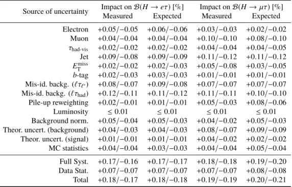
`τ`0non-VBF are due to the looser selection criteria defined for the former channel (Section 5). Table 6 shows a summary of the uncertainties on
B(H→`τ). The uncertainties associated with mis-identified leptons/jets and those related to the jet energy scale and resolution exhibit the highest impact on the best-fit branching ratios in both searches. The combined impact from full systematic uncertainties and data statistics ranges from 0
.17% to 0
.19% on the measurements.
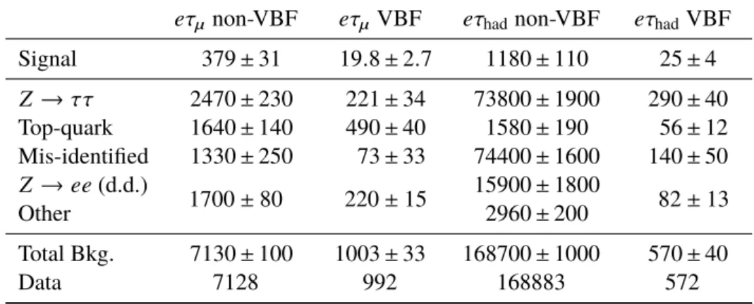
Table 4: Event yields and predictions as computed by the background-only fit in different signal regions of the H→eτanalysis. Uncertainties include both statistical and systematic contributions. “Other” contains di-boson, Z → ``,H → ττandH →WW background processes. For theeτhad channel theZ → ee(d.d.) component corresponds to electrons mis-identified asτhad-vis. This contribution is summed with “Other” due to the lack of statistics in the VBF category. The uncertainty on the total background includes all correlations between channels.
The normalizations of top-quark (`τ`0channel only) andZ→ττbackground components are determined by the fit, while the expected signal event yields are given forB(H→eτ)=1%.
eτµ
non-VBF
eτµVBF
eτhadnon-VBF
eτhadVBF
Signal 379
±31 19
.8
±2
.7 1180
±110 25
±4
Z →ττ
2470
±230 221
±34 73800
±1900 290
±40
Top-quark 1640
±140 490
±40 1580
±190 56
±12
Mis-identified 1330
±250 73
±33 74400
±1600 140
±50
Z →ee(d.d.)
1700
±80 220
±15 15900
±1800
82
±13
Other 2960
±200
Total Bkg. 7130
±100 1003
±33 168700
±1000 570
±40
Data 7128 992 168883 572
Table 5: Event yields and predictions as computed by the background-only fit in different signal regions of the H→µτanalysis. Uncertainties include both statistical and systematic contributions. “Other” contains di-boson, Z → ``,H → ττandH → WWbackground processes. The uncertainty on the total background includes all correlations between channels. The normalizations of top-quark (`τ`0 channel only) and Z → ττ background components are determined by the fit, while the expected signal event yields are given forB(H→ µτ)=1%.
µτe
non-VBF
µτeVBF
µτhadnon-VBF
µτhadVBF
Signal 287
±23 14
.6
±1
.9 1200
±120 25
±5
Z →ττ
1860
±130 144
±26 96100
±2000 274
±33
Top-quark 1260
±130 390
±34 1620
±210 51
±10
Mis-identified 1340
±210 41
±21 63900
±1600 149
±33
Other 1180
±140 168
±18 23000
±1000 104
±15
Total Bkg. 5640
±100 743
±29 184500
±1200 580
±30
Data 5664 723 184508 583
Table 6: Summary of the sources of systematic uncertainties and their impact on the best-fit value ofBin theH→eτ andH→µτsearches. The measured values are obtained by the fit to data, while the expected ones are determined by the fit to a background-only sample.
Source of uncertainty Impact onB(H→eτ)[%] Impact onB(H→ µτ)[%]
Measured Expected Measured Expected
Electron +0.05/−0.05 +0.06/−0.06 +0.03/−0.03 +0.02/−0.02 Muon +0.04/−0.04 +0.04/−0.04 +0.10/−0.10 +0.08/−0.10 τhad-vis +0.02/−0.02 +0.02/−0.02 +0.04/−0.04 +0.04/−0.05 Jet +0.09/−0.08 +0.09/−0.09 +0.11/−0.12 +0.11/−0.12 Emiss
T +0.02/−0.02 +0.02/−0.03 +0.05/−0.08 +0.03/−0.05 b-tag +0.02/−0.03 +0.03/−0.03 +0.01/−0.01 +0.01/−0.01 Mis-id. backg. (`τ`0) +0.08/−0.07 +0.09/−0.08 +0.07/−0.07 +0.07/−0.07 Mis-id. backg. (`τhad) +0.12/−0.11 +0.11/−0.12 +0.11/−0.11 +0.10/−0.10 Pile-up reweighting +0.02/−0.01 +0.01/−0.01 +0.05/−0.03 +0.08/−0.06
Luminosity ≤0.01 ≤0.01 ≤0.01 ≤0.01 Background norm. +0.05/−0.04 +0.05/−0.03 +0.04/−0.02 +0.05/−0.03 Theor. uncert. (background) +0.04/−0.03 +0.04/−0.03 +0.08/−0.07 +0.09/−0.09 Theor. uncert. (signal) +0.01/−0.01 +0.01/−0.01 +0.04/−0.02 +0.02/−0.02 MC statistics +0.04/−0.04 +0.03/−0.03 +0.04/−0.04 +0.05/−0.04 Full Syst. +0.17/−0.16 +0.17/−0.17 +0.18/−0.18 +0.19/−0.20 Data Stat. +0.07/−0.07 +0.07/−0.07 +0.07/−0.07 +0.08/−0.08 Total +0.18/−0.17 +0.18/−0.18 +0.19/−0.19 +0.20/−0.21
BDT Score 1
− −0.8−0.6 −0.4 −0.2 0 0.2 0.4 0.6 0.8 1
Data / Pred.
0.5 0.75 1 1.25 1.5
Events / 0.10
1 10 102
103
104
ATLAS Preliminary = 13 TeV, 36.1 fb-1
s LFV eτ
non-VBF τµ
e
Data Sig. (B=1%)×10 Mis-id. Z→ττ
Top Other
Uncert.
BDT Score 1
− −0.8−0.6 −0.4 −0.2 0 0.2 0.4 0.6 0.8 1
Data / Pred.
0.5 0.75 1 1.25 1.5
Events / 0.10
1 10 102
103
104 ATLAS Preliminary = 13 TeV, 36.1 fb-1
s LFV eτ
µ VBF eτ
Data Sig. (B=1%)×10 Mis-id. Z→ττ
Top Other
Uncert.
BDT Score 1
− −0.8−0.6 −0.4 −0.2 0 0.2 0.4 0.6 0.8 1
Data / Pred.
0.8 0.9 1 1.1 1.2
Events / 0.10
1 10 102
103
104
105
106
107
ATLAS Preliminary = 13 TeV, 36.1 fb-1
s LFV eτ
non-VBF τhad
e
Data Sig. (B=1%)×10 Mis-id. Z→ττ Top Z→ee (d.d.) Other Uncert.
BDT Score 1
− −0.8−0.6 −0.4 −0.2 0 0.2 0.4 0.6 0.8 1
Data / Pred.
0.5 0.75 1 1.25 1.5
Events / 0.10
1 10 102
103
104 ATLAS Preliminary = 13 TeV, 36.1 fb-1
s LFV eτ
had VBF eτ
Data Sig. (B=1%)×10 Mis-id. Z→ττ
Top Other
Uncert.
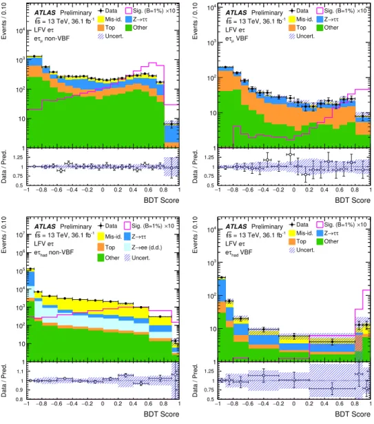
Figure 2: BDT score distributions after the background+signal fit in each signal region of theeτsearch, but with the LFV signal overlaid, normalized withB(H→eτ)=1% and enhanced by a factor 10 for visibility. The top and bottom plots displayeτµandeτhadBDT scores respectively, whereas the left (right) column corresponds to the non-VBF (VBF) category. The size of the combined statistical, experimental and theoretical uncertainties in the background is indicated by the hatched bands. The binning is shown as in the statistical analysis.
BDT Score 1
− −0.8−0.6 −0.4 −0.2 0 0.2 0.4 0.6 0.8 1
Data / Pred.
0.5 0.75 1 1.25 1.5
Events / 0.10
1 10 102
103
104
ATLAS Preliminary = 13 TeV, 36.1 fb-1
s τ LFV µ
non-VBF τe
µ
Data Sig. (B=1%)×10 Mis-id. Z→ττ
Top Other
Uncert.
BDT Score 1
− −0.8−0.6 −0.4 −0.2 0 0.2 0.4 0.6 0.8 1
Data / Pred.
0.5 0.75 1 1.25 1.5
Events / 0.10
1 10 102
103
104
ATLAS Preliminary = 13 TeV, 36.1 fb-1
s τ LFV µ
e VBF τ µ
Data Sig. (B=1%)×10 Mis-id. Z→ττ
Top Other
Uncert.
BDT Score 1
− −0.8−0.6 −0.4 −0.2 0 0.2 0.4 0.6 0.8 1
Data / Pred.
0.8 0.9 1 1.1 1.2
Events / 0.10
1 10 102
103
104
105
106
107 ATLAS Preliminary = 13 TeV, 36.1 fb-1
s τ LFV µ
non-VBF τhad
µ
Data Sig. (B=1%)×10 Mis-id. Z→ττ
Top Other
Uncert.
BDT Score 1
− −0.8−0.6 −0.4 −0.2 0 0.2 0.4 0.6 0.8 1
Data / Pred.
0.5 0.75 1 1.25 1.5
Events / 0.10
1 10 102
103
104 ATLAS Preliminary = 13 TeV, 36.1 fb-1
s τ LFV µ
had VBF τ µ
Data Sig. (B=1%)×10 Mis-id. Z→ττ
Top Other
Uncert.
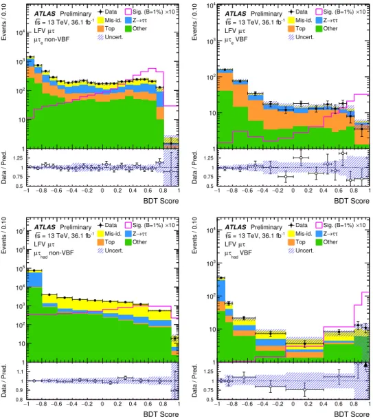
Figure 3: BDT score distributions after the background+signal fit in each signal region of theµτsearch, but with the LFV signal overlaid, normalized withB(H→ µτ)=1% and enhanced by a factor 10 for visibility. The top and bottom plots displayµτeandµτhadBDT scores respectively, whereas the left (right) column corresponds to the non-VBF (VBF) category. The size of the combined statistical, experimental and theoretical uncertainties in the background is indicated by the hatched bands. The binning is shown as in the statistical analysis. In the data/background prediction ratio plots, points outside the displayedy-axis range are shown by arrows.
9 Results
The best-fit branching ratios and upper limits are computed under the assumption of
B(H → µτ) =0 for the
H→eτsearch and
B(H→eτ)=0 for the
H →µτsearch, respectively. The best-fit values of the LFV Higgs boson branching ratios are equal to 0
.15
+0−0..1817% and
−0
.22
±0
.19% for the
H →eτand
H→ µτsearch, respectively. In the absence of any significant excess, upper limits on the LFV branching ratios are set for a Higgs boson with
mH =125 GeV. The observed (median expected) 95% CL upper limits are 0
.47% (0
.34
+0−0..1310%) and 0
.28% (0
.37
+0−0..1410%) for the
H →eτand
H → µτsearches, respectively.
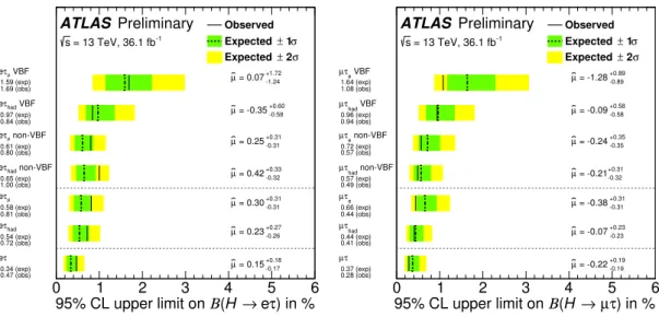
These limits are significantly lower than the corresponding Run 1 limits of Refs. [7, 8]. The breakdown of contributions from different signal regions is shown in Fig. 4.
) in % eτ H → ( Β 95% CL upper limit on
0 1 2 3 4 5 6
ATLAS Preliminary Observed 1σ Expected ±
2σ Expected ± = 13 TeV, 36.1 fb-1
s
µ VBF τ e
1.59 (exp) 1.69 (obs)
-1.24 +1.72
= 0.07 µ
τµ e
0.58 (exp) 0.81 (obs)
-0.31 +0.31
= 0.30 µ
τhad e
0.54 (exp) 0.72 (obs)
-0.26 +0.27
= 0.23 µ non-VBF
τhad e
0.65 (exp) 1.00 (obs)
-0.32 +0.33
= 0.42 µ non-VBF
τµ e
0.61 (exp) 0.80 (obs)
-0.31 +0.31
= 0.25 µ
τ e
0.34 (exp) 0.47 (obs)
-0.17 +0.18
= 0.15 µ
had VBF eτ
0.97 (exp) 0.84 (obs)
-0.58 +0.60
= -0.35 µ
) in % τ µ H → ( Β 95% CL upper limit on
0 1 2 3 4 5 6
ATLAS Preliminary Observed 1σ Expected ±
2σ Expected ± = 13 TeV, 36.1 fb-1
s
e VBF τ µ 1.64 (exp) 1.08 (obs)
-0.89 +0.89
= -1.28 µ
τe µ 0.66 (exp) 0.44 (obs)
-0.31 +0.31
= -0.38 µ
τhad µ 0.44 (exp) 0.41 (obs)
-0.23 +0.23
= -0.07 µ non-VBF
τhad µ 0.57 (exp) 0.49 (obs)
-0.32 +0.31
= -0.21 µ non-VBF
τe µ 0.72 (exp) 0.57 (obs)
-0.35 +0.35
= -0.24 µ
τ µ 0.37 (exp) 0.28 (obs)
-0.19 +0.19
= -0.22 µ
had VBF τ µ 0.96 (exp) 0.94 (obs)
-0.58 +0.58
= -0.09 µ
Figure 4: 95% CL upper limits on the LFV branching ratios of the Higgs boson,H→eτ(left) andH→ µτ(right).
Best-fit values of the branching ratios ( ˆµ) are also given, in %. The limits are computed under the assumption that eitherB(H → µτ) =0 (left) orB(H → eτ) =0 (right). Results of the fit when only the data of an individual channel or of an individual category are used, are also shown; in these cases the signal and control regions from all other channels/categories are removed from the fit.
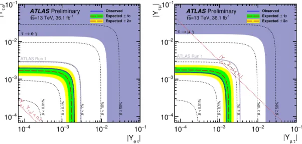
The branching ratio of the LFV Higgs decay is related to the non-diagonal Yukawa coupling matrix elements [84] by the formula
p|Y`τ|2+|Yτ`|2=
8
π mHB(H→`τ)
1
− B(H→`τ)ΓH(SM
),(1) where
ΓH(SM
)stands for the Higgs boson width as predicted by the Standard Model. Thus, the observed limits on the branching ratio correspond to the following limits on the matrix elements:
p|Yτe|2+|Yeτ|2 <
0
.00197, and
q|Yτµ|2+|Yµτ|2<