Estimation of non-prompt and fake lepton backgrounds in final states with top quarks produced in proton-proton collisions at √

(1)

ATLAS-CONF-2014-058 01October2014

ATLAS NOTE

ATLAS-CONF-2014-058

September 30, 2014

Estimation of non-prompt and fake lepton backgrounds in final states with top quarks produced in proton-proton collisions at √

s = 8 TeV with the ATLAS detector

The ATLAS Collaboration

Abstract

This note presents methods for estimating non-prompt and fake lepton backgrounds de- veloped in the context of top analyses using the ATLAS detector. The analysis is performed on the ATLAS 2012 proton-proton collision data sample, collected at the LHC, correspond- ing to a luminosity of 20.3 fb

⁻¹

at

√

s

=

8 TeV. Final states with lepton

+

jets and dilepton events are considered. Two different data-driven methods are described and compared. The first method (matrix method) is based on the measurement of efficiencies of leptons with re- laxed identification criteria. The second one (fitting method) is based on the construction of templates for non-prompt and fake leptons. For final states with two leptons, the systematic uncertainties of the estimates using the matrix method are 30-100%. For final states with one lepton, the two methods give consistent results within systematic uncertainties, which are 10-50% for the matrix method and 50% for the fitting method.

c

Reproduction of this article or parts of it is allowed as specified in the CC-BY-3.0 license.

(2)

1 Introduction

The selection of events with top quarks is often based on the identification of one or more charged isolated leptons from the decay of W or Z bosons, referred to as ‘prompt’ or ‘real’ leptons in the following.

Acceptance, quality and isolation requirements are applied to select these leptons.

Non-prompt leptons and non-leptonic particles may satisfy these selection criteria, giving rise to so called ‘non-prompt and fake’ lepton backgrounds. In the case of electrons, these include contributions from semileptonic decays of b- and c-quarks, photon conversions and jets with large electromagnetic energy (from the hadronisation to

π⁰

’s or from early showering in the calorimeter). Non-prompt or fake muons can originate from semileptonic decays of b- and c-quarks, from charged hadron decays in the tracking volume or in hadronic showers, or from punch-through particles emerging from high-energy hadronic showers. For analyses based on events with one lepton, this background stems from multi- jet events, characterised by a cross-section several orders of magnitude larger than for W boson or top events. In events with two leptons the non-prompt and fake lepton backgrounds are dominated by W

+jets

and semileptonic t¯ t events, with a fake lepton in addition to the real one, and more rarely events with two fake leptons.

These backgrounds are estimated using data-driven techniques. The most common methods are called matrix, jet-lepton and anti-lepton methods (these latter two are referred to in the following as

‘fitting methods’) and have been used for ATLAS early top quark studies [1,

2]. All these techniques

were also applied on more recent 7 TeV analyses in t¯ t dilepton studies [3] or single top measurements [4].

This note presents a survey of these methods and their application with 8 TeV data. New methods are also developed in the context of t¯ t dilepton analyses with 8 TeV data [5,

6].

Results are presented on typical top selections such as the t¯ t semileptonic and the dileptonic selec- tions. The analysis is performed in the ATLAS 2012 proton-proton collision data sample, corresponding to an integrated luminosity of 20.3 fb

⁻¹

at

√

s

=

8 TeV.

2 The ATLAS detector

The ATLAS detector [7] consists of four main subsystems: an inner tracking system surrounded by a superconducting solenoid, electromagnetic and hadronic calorimeters, and a muon spectrometer. The inner detector provides tracking information from pixel and silicon microstrip detectors in the pseudo- rapidity

¹

range

|η| <2.5 and from a transition radiation tracker (TRT) covering |η| <2.0, all immersed

in a 2 T magnetic field provided by a superconducting solenoid. The electromagnetic (EM) sampling calorimeter uses lead and liquid argon (LAr) and is divided into a barrel region (|η|

<1.475) and an

end-cap region (1.375<

|η| <3.2). Hadron calorimetry is based on two diff

erent detector technologies, with scintillator tiles or LAr as active media, and with either steel, copper, or tungsten as the absorber material. The calorimeters cover

|η| <4.9. The muon spectrometer measures the deflection of muon

tracks within

|η|<2.7 using multiple layers of high-precision tracking chambers located in toroidal fields

of approximately 0.5 T and 1 T in the central and end-cap regions of ATLAS, respectively. The muon spectrometer is also instrumented with separate trigger chambers covering

|η|<2.4.

1ATLAS uses a right-handed coordinate system with its origin at the nominal interaction point (IP) in the centre of the detector and thez-axis coinciding with the axis of the beam pipe. Thex-axis points from the IP to the centre of the LHC ring, and they-axis points upward. Cylindrical coordinates (r,φ) are used in the transverse plane,φbeing the azimuthal angle around the beam pipe. The pseudorapidity is defined in terms of the polar angleθasη =−lnθ/2. For the purpose of the fiducial selection, this is calculated relative to the geometric centre of the detector; otherwise, it is relative to the reconstructed primary vertex of each event.

(3)

3 Simulation samples

Various Monte Carlo (MC) samples are used in the analysis. Simulated t¯ t events are generated using the

POWHEG

generator v1 r2129 [8,

9], which implements the NLO matrix element for inclusive

t¯ t pro- duction, with the HERAPDF15NLO [10] parton distribution functions (PDFs).

POWHEG

is interfaced to

PYTHIA

v6.425 [11] with the CTEQ6L1 PDF set and the corresponding Perugia2011C tune [12]. The renormalisation and factorisation scales [13] are calculated event-by-event using Q

² =

m

²_t +

p

²_T

, where m

t

and p

_T

are the top quark mass and the top quark transverse momentum. The top quark mass is as- sumed to be 172.5 GeV. Another t¯ t sample, used for studies of systematic uncertainties, uses CT10 [14]

PDFs.

PYTHIA

v6.425 with the AUET2B tune [15] is used for hadronisation and to describe the un- derlying event. The t¯ t cross-section for pp collisions at a centre-of-mass energy of

√

s

=

8 TeV is

σtt¯=

253

⁺₋₁₆¹⁵

pb. It has been calculated at next-to-next-to leading order (NNLO) in QCD including re- summation of next-to-next-to-leading logarithmic (NNLL) soft gluon terms with top

++

2.0 [16–22]. The PDF and

αS

uncertainties were calculated using the PDF4LHC prescription [23] with the MSTW2008 68% CL NNLO [24,25], CT10 NNLO [14,

26] and NNPDF2.3 5f FFN [27] PDF sets and these are added

in quadrature to the scale uncertainty.

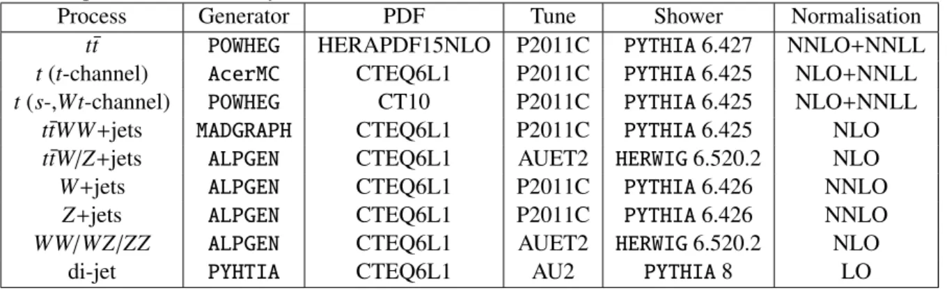
Table 1: A summary of generators, PDF sets and cross-section calculations used for the various simu- lated samples used in the analysis.

Process Generator PDF Tune Shower Normalisation

t¯ t

POWHEG

HERAPDF15NLO P2011C

PYTHIA

6.427 NNLO

+

NNLL

t (t-channel)

AcerMC

CTEQ6L1 P2011C

PYTHIA

6.425 NLO

+

NNLL

t (s-,Wt-channel)

POWHEG

CT10 P2011C

PYTHIA

6.425 NLO+NNLL

t¯ tWW

+

jets

MADGRAPH

CTEQ6L1 P2011C

PYTHIA

6.425 NLO t¯ tW/Z

+

jets

ALPGEN

CTEQ6L1 AUET2

HERWIG

6.520.2 NLO

W

+jets ALPGEN

CTEQ6L1 P2011C

PYTHIA

6.426 NNLO

Z

+

jets

ALPGEN

CTEQ6L1 P2011C

PYTHIA

6.426 NNLO

WW/WZ/ZZ

ALPGEN

CTEQ6L1 AUET2

HERWIG

6.520.2 NLO

di-jet

PYHTIA

CTEQ6L1 AU2

PYTHIA

8 LO

Samples of single top quark backgrounds corresponding to the s-channel and Wt production mech- anisms are generated with

POWHEG

using the CT10 set of PDF, while for the t-channel

AcerMC

[28]

using the CTEQ6L1 set of PDF. All samples are interfaced to

PYTHIA

set of PDF and Perugia P2011C tune. Overlaps between the t¯ t and Wt final states are removed using the so-called diagram removal scheme [29]. The single top quark cross-sections are normalised to the approximate NLO

+

NNLL QCD cross-sections [30,

31] using the MSTW2008 NNLO PDF.

Samples of W

/

Z

+jet events are generated using theALPGEN

v2.14 [32] LO generator and the

CTEQ6L1

PDF set [33]. Parton shower and fragmentation are modeled with

PYTHIA

v6.425. To avoid double-

counting of partonic configurations generated by both the matrix-element calculation and the parton-

shower evolution, a parton-jet matching scheme (MLM matching) [34] is employed. The W

/

Z

+jet sam-

ples are generated with up to five additional partons, separately for W

/

Z

+

light jets, W

/

Z

+

b b ¯

+

jets and

W

/

Z

+

c c ¯

+jets. The overlap between

W

/

Z

+

Q Q(Q ¯

=

b, c) events generated from the matrix element

calculation and those generated from parton-shower evolution in the W

/

Z

+light jet samples is avoided

via an algorithm based on the angular separation between the extra heavy-quarks: if

∆

R(Q, Q) ¯

>

0.4,

the matrix-element prediction is used, otherwise the parton-shower prediction is used. For assessment

of systematic uncertainties, W

/

Z

+jet samples are also generated usingSHERPA

v1.4.1 [35], for the hard

process, the parton shower and hadronisation, and the underlying event, with the CT10 PDF set. The

(4)

inclusive cross-sections of W

/

Z-boson production are calculated to NNLO with FEWZ [36] with an un- certainty of

±4%. For the

W

+

jets and Z

+

jets backgrounds in association with two additional jets the uncertainty is conservatively estimated from the Berends-Giele scaling [37,

38] (W+n+1/W+n) and this

yields

±34%

The ZZ/γ

^∗

, WZ/γ

^∗

and WW

+

jets samples are generated using

ALPGEN+HERWIG

with up to three ad- ditional partons. They are normalised to the NLO QCD cross-section prediction using the MSTW2008NLO set.

The samples of t¯ t

+

Z(

+

jets) and t¯ t

+

W(

+

jets) production are generated with

ALPGEN

with AUET2 tune, while the t¯ t

+

WW sample is generated with

MADGRAPH

[39] interfaced to

PYTHIA

with CTEQ6L1 PDFs. They are normalised to NLO cross-section predictions [6].

A sample of di-jet events is also used in the following, to derive one of the templates for the non- prompt and fake lepton background and to perform MC-simulation based studies on the non-prompt and fake lepton composition. This sample is simulated with

PYTHIA

v8 [40] and includes all the relevant 2

→

2 QCD processes, filtered at truth level to mimic a level-1 electromagnetic trigger requirement.

All

PYTHIA6

samples use

PHOTOS

v2.15 [41] to simulate photon radiation and

TAUOLA

v1.20 [42] to simulate

τ

decays. The simulated events are weighted such that the distribution of the average number of pp interactions per bunch crossing agrees with data. All samples are processed through a simulation [43]

of the detector geometry and response using

GEANT4

[44]. Table

1

provides a summary of the MC samples used in the analysis. All simulated samples are processed through the same reconstruction software as the data.

To improve the W/Z

+

jets background modeling, the simulated W/Z p

_T

spectrum is reweighted to match the one reconstructed in data. In addition the yields of ZQ Q(Q ¯

=

b, c) are also corrected to match the observed one (see Ref. [6]).

4 Object reconstruction

Electron candidates [45] are reconstructed from isolated electromagnetic calorimeter energy deposits matched to inner detector tracks and passing identification requirements, with transverse energy E

_T>

25 GeV and pseudorapidity

|η_cluster| <2.47 (whereη_cluster

is the pseudorapidity of the calorimeter clus- ter associated with the electron candidate). Those within the transition region between the barrel and end-cap electromagnetic calorimeters, 1.37

< |η_cluster| <

1.52, are removed. Isolation requirements are used to reduce backgrounds from non-prompt and fake electrons, by applying cuts on the calorimeter transverse energy within a cone of size

∆

R

= p

(∆

η)²+

(∆

φ)² <

0.2 and the scalar sum of track trans- verse momentum p

_T

within

∆

R

<

0.3, in each case excluding the contribution from the electron itself.

These two quantities are each required to be smaller than E

_T

and

η-dependent thresholds calibrated to

separately give nominal selection efficiencies of 90% for prompt electrons from Z

→

ee decays. Electron candidates passing tight [45] selection criteria and the isolation requirements are referred to as tight elec- trons. Loose electrons are electrons satisfying tight [45] selection criteria but where the requirements on TRT-based particle identification and on the energy-to-momentum ratio E/p are relaxed and no requests on the isolation are made.

Muon candidates are reconstructed by combining matching tracks reconstructed in both the inner detector and muon spectrometer [46], and required to satisfy p

_T>25 GeV and|η| <2.5. Isolation re-

quirements are also introduced, asking for I

<

0.05, where I is the ratio of the sum of track p

_T

in a variable-sized cone of radius

∆

R

=

10 GeV/ p

^µ_T

to the transverse momentum p

_T

of the muon. These muons are referred to as ‘tight muons’. For loose muons, no request on the isolation is made but all other selection requirements are applied.

The probability that a lepton from a W

/

Z decay (non-prompt or fake lepton) identified as a loose

lepton satisfies the tight identification criteria is defined ‘real efficiency’

ε_r

, and ‘fake efficiency’ as

ε_f

(5)

respectively.

Jets are reconstructed with the anti-k

t

algorithm [47,

48] with radius parameter

R

=

0.4, starting from calorimeter energy clusters calibrated using the local cluster weighting method [49]. Jets are calibrated using an energy- and

η-dependent simulation-based calibration scheme, with in-situ corrections based

on data, and are required to satisfy p

_T>25 GeV and|η| <2.5. To suppress the contribution from low-p_T

jets originating from pileup interactions, a validation based on tracks that the jet comes from the primary vertex is applied to jets with p

_T<50 GeV and|η|<2.4: jets are required to have at least 50% of the scalar

sum of the p

_T

of tracks associated to the jet coming from tracks associated to the event primary vertex.

The primary vertex is defined as the reconstructed vertex with the highest sum of associated track p

²_T

. During jet reconstruction, no distinction is made between identified electrons and jet energy deposits.

Therefore, if any of the jets lie within

∆

R

<

0.2 of a selected electron, the closest jet is discarded in order to avoid double-counting of electrons as jets. Finally, to further suppress non-isolated leptons from heavy-flavour decays inside jets, electrons and muons within

∆

R

<

0.4 of selected jets are also discarded.

This procedure is repeated separately for the loose and tight leptons.

Jets are identified as containing a b-quark (b-tagged) via an algorithm [50] using multivariate tech- niques to combine information from the impact parameters of displaced tracks as well as topological properties of secondary and tertiary decay vertices reconstructed within the jet. The working point used for this measurement corresponds to 70% e

ffi

ciency to tag a b-quark jet, with a light-jet rejection fac- tor of

∼130 and a charm jet rejection factor of 5, as determined for

b-tagged jets with p

_T>20 GeV and

|η| <2.5 in simulated

t¯ t events. The e

ffi

ciency of the the b-tagging algorithm is measured for each jet flavour using control samples in data and compared to the simulation. In the case of b-jets, scale factors are estimated based on observed and simulated b-tagging rates in t¯ t events [51]. In the case of c-jets, they are derived based on jets with identified D mesons [52]. In the case of light-flavour jets, scale factors are derived using dijet event [53].

The missing transverse energy is reconstructed from the vector sum of all calorimeter cell ener- gies associated with topological clusters with

|η| <4.5 [54]. Contributions from the calorimeter clusters

matched with either a reconstructed lepton or jet are corrected to the corresponding energy scale. The term accounting for the selected muon p

_T

is included into the calculation. The symbol E

_T^miss

is used for its magnitude.

5 Event selection

Events are required to pass either a single electron or single muon trigger. The p

_T

thresholds are 24 or 60 GeV for electrons (labelled e24vhi and e60) and 24 or 36 GeV for muons (labelled mu24i and mu36). The triggers with the lower p

_T

threshold include isolation requirements on the candidate lepton that are looser than those applied for the identification of tight leptons. Additional pre-scaled triggers without isolation requirements (e24vh and mu24) are considered in the following, but are not used to select events unless specified.

The events selected to study top quark pair and single top production in the lepton+jets and dilep- ton channels have one or two leptons (electrons or muons), a significant amount of missing transverse energy and a number of jets and b-jets In the lepton+jets channels (e

+jets and µ+jets), the presence

of exactly one loose or tight electron or muon is required. In the following, when not specified, a tight lepton is required. To suppress the non-prompt and fake lepton backgrounds, besides the cut in E

^miss_T

, a cut on the transverse mass of the lepton and E

^miss_T

can be introduced. It is defined as m

^W_T = q

2p

^lepton_T

E

^miss_T

(1

−

cos

∆φ), where∆φ

is the difference in azimuthal angle between the lepton

and E

_T^miss

. The dileptonic event selection typically requires the presence of two opposite-sign charge

(OS) leptons, and, in case of the eµ channel (which is the only dilepton channel where results are pre-

(6)

sented here) a cut on the sum of the p

_T

of leptons and jets in the event, a quantity referred to as H

_T

in the following. Details of the t¯ t semileptonic and dileptonic event selections can be found in Ref. [55]. In what follows, if the quality of the leptons is not specified, the two leptons are required to be tight.

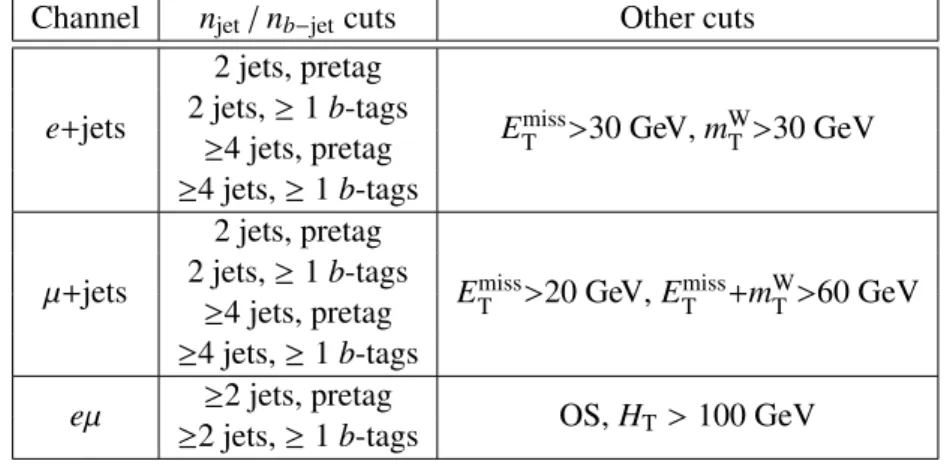
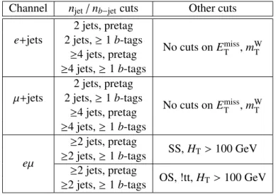
Table 2: Summary of the signal regions considered in the analysis. The term ‘pretag’ is used to indicate that no requirements on the number of b-jets are applied, while ‘OS’ stands for opposite sign charged leptons.

Channel n

_jet/

n

_b−jet

cuts Other cuts e

+jets

2 jets, pretag

E

^miss_T >30 GeV,

m

^W_T>30 GeV

2 jets,

≥

1 b-tags

≥4 jets, pretag

≥4 jets,≥

1 b-tags

µ+jets

2 jets, pretag

E

_T^miss>20 GeV,

E

^miss_T +

m

^W_T>60 GeV

2 jets,

≥

1 b-tags

≥4 jets, pretag

≥4 jets,≥

1 b-tags eµ

≥2 jets, pretag

OS, H

_T>

100 GeV

≥2 jets,≥

1 b-tags

In the presented analysis, for each of the considered lepton+jets or dilepton channels, different signal regions are defined by the requirements summarised in Table

2. These are typical regions where the

t¯ t signal is extracted, or, in case of the two-jet regions, the dominant real lepton background from W

+

jets is controlled. Here and in the following, the term ‘pretag’ is used to refer to a region without any requirement on the number of b-jets, i.e events with 0, 1 or at least 2 b-jets.

6 Matrix method

6.1 Overview

In a data sample containing events with a single lepton, the number of events with one tight lepton (N

^t

) and the number of events with one loose lepton (N

^l

) can be expressed as linear combinations of the number of events with a real or a non-prompt or fake lepton:

N

^l =

N

_r^l+

N

_f^l,

N

^t = ε_r

N

_r^l+ε_f

N

_f^l,

(1)

where

ε_r

is the fraction of real leptons in the loose selection that also pass the tight one and

ε_f

is the frac- tion of non-prompt and fake lepton backgrounds in the loose selection that also pass the tight selection.

If

ε_r

and

ε_f

are known, the number of events with a non-prompt or fake lepton can be calculated from Eq.

1

given the measured N

^l

and N

^t

. The relative efficiencies

ε_r

and

ε_f

are measured in data in control samples enriched in either real or non-prompt or fake lepton. The number of tight events coming from non-prompt or fake lepton backgrounds can be expressed as:

N

_f^t = ε_f

ε_r−ε_f

(ε

_r

N

^l−

N

^t

). (2)

The matrix method e

ffi

ciencies

εr

and

εf

depend on lepton kinematics and event characteristics,

such as and the number of jets or b-jets. To correctly account for this, an event weight is computed

(7)

from the efficiencies, which are parametrised as a function of the various object kinematics (as detailed Section

6.2):

wi = ε_f

ε_r−ε_f

(ε

_r−δ_i

), (3)

where

δi

equals unity if the loose event i passes the tight event selection and 0 otherwise. The background estimate in a given bin of the final observable is given by the sum of

wi

over all events in that bin.

In the case of a dilepton selection, the numbers of observed events with two tight leptons (denoted as N

_tt

), one loose and one tight lepton (N

tl

and N

_lt

) or two loose leptons (N

ll

) are counted. Here and in what follows, the leptons are ordered by p

_T

in the indexes, such that the leading lepton in N

_tl

region is tight and the leading lepton in N

_lt

is loose. Using

ε_r

and

ε_f

, already defined for the single lepton case, linear equations are obtained for the observed yields as a function on the number of events with zero, one and two real leptons together with two, one and zero non-prompt or fake leptons (N

_ff

, N

_rf

, N

_fr

and N

_fr

respectively):







N

_rr

N

_fr

N

_rf

N

_ff







=M⁻¹







N

_tt

N

_tl

N

_lt

N

_ll







,

(4)

where

M

is a 4

×

4 matrix written in terms of

ε_r

and

ε_f

. It is calculated as:

M=







ε_r,1ε_r,2 ε_r,1ε_f,2 ε_f,1ε_r,2 ε_f,1ε_f,2 ε_r,1ε_r,2 ε_r,1ε_f,2 ε_f,1ε_r,2 ε_f,1ε_f,2 εr,1εr,2 εr,1εf,2 εf,1εr,2 εf,1εf,2

ε_r,1ε_r,2 ε_r,1ε_f,2 ε_f,1ε_r,2 ε_f,1ε_f,2







,

(5)

where the index on

ε_r

and

ε_f

refers to the first (1) or second (2) lepton in the event, and ¯

ε

stands for (1

−ε). Similarly to the single lepton case, four weights,wrr

,

wr f

,

wf r

and

wf f

are calculated on event- by-event basis. The probability that an event with two loose leptons contains at least one non-prompt or fake lepton is then given by

w_rf+w_fr+w_ff

. Finally, the estimated background contribution in a sample of events with two tight leptons is given by the event weight:

w_tt = ε_r,1ε_f,2w_rf+ε_f,1ε_r,2w_fr+ε_f,1ε_f,2w_ff.

(6) 6.2 Measurement and parametrisation of the e ffi ciencies

Real and fake e

ffi

ciencies

ε_r

and

ε_f

are measured in control regions which are representative of the signal regions in terms of kinematics and, in the case of the fake e

ffi

ciency, non-prompt and fake lepton background composition. Table

3

summarises the definition of the different control regions used to extract the real and fake e

ffi

ciencies, as explained in the following.

The real e

ffi

ciencies

ε_r

are measured using the tag-and-probe method from the Z→ ee and Z→

µµ

control regions. This method selects an unbiased sample of loose leptons (probes) from the Z boson decay by using a tight selection requirement on the other object produced from the particle’s decay (tags). The e

ffi

ciency is determined by applying the tight selection to the probe lepton. For each pair, the tag and the probe leptons are required to have opposite reconstructed charges. A typical dilepton invariant mass range used in this analysis is 80 to 100 GeV, although this range is varied in systematic studies. After this selection, the sample still contains non-prompt and fake lepton backgrounds. The background is determined using a side band subtraction approach and is found to be at the percent level.

In the case of electrons, for which the identification is more sensitive to jet activity in the event,

εr

is

corrected to match the expected e

ffi

ciency in t¯ t events. The correction is calculated from comparisons of

(8)

Table 3: Summary of the different control regions used to extract the matrix method efficiencies. The term ‘pretag’ is used to indicate that no requirements on the number of b-jets are applied, while ‘OS’

stays for opposite-sign charge leptons.

Channel n

_jet/

n

b−jet

cuts Other cuts Used for

e

+jets ≥

1 jets, pretag m

^W_T<20 GeV,

E

^miss_T +

m

^W_T<60 GeV ε_f

(e) extraction

µ+

jets

≥1 jets, pretag |d^sig₀ | >

5

ε_f

(µ) extraction ee

≥1 jets, pretag

OS, 80 GeV

<

m

_ee<

100 GeV

ε_r

(e) extraction

µµ ≥

1 jets, pretag OS, 80 GeV

<

m

_µµ<

100 GeV

ε_r

(µ) extraction

values determined in t¯ t and Z simulated events. This correction is derived separately for each of the bins where

ε_r

is measured (see later in the text) and is on average -3%.

The fake e

ffi

ciencies

ε_f

are measured in data samples dominated by non-prompt and fake lepton background events. These control regions, denoted CR

_f

, contain only one loose lepton, at least one jet and have low E

_T^miss

and/or m

^W_T

or high lepton impact parameter. Distributions of the variables used to de- fine CR

_f

are shown in Fig.

1. For

e

+

jets events CR

_f

is defined by m

^W_T <

20 GeV & m

^W_T +

E

^miss_T <

60 GeV.

For

µ+jets events CRf

is defined by

|d^sig₀ | >

5, where d

₀^sig

is the muon impact parameter significance, d

₀^sig =

d

₀/√

err(d

0

). In the case of muons, a linear extrapolation of the dependence on d

₀^sig

from CR

f

to the inclusive selection is performed. The result of this extrapolation is an overall increase of up to 5%, depending on the number of b-jets and the trigger (see later). The contribution from processes containing prompt leptons, such as Z

+

jets, W

+

jets, t¯ t, single top and diboson, are determined using MC simulation.

In events with one tight electron (muon), the contamination from these processes is of order 50% (15%).

Efficiencies are determined as the ratio between the number of tight and loose events in these regions.

One of the two triggers used to select events has an isolation requirement, while loose leptons are defined without any isolation cut. E

ffi

ciencies are therefore expected to be di

ff

erent for leptons matched to the trigger with or without isolation. Efficiencies are thus derived and applied depending on the trigger being fired by the lepton (see section

5) and on the lepton

p

_T

being below or above the high-p

T

trigger threshold. E

ffi

ciencies extracted in the case of the e24vh (mu24) trigger are used in the dilepton channel for electrons (muons) below the high- p

_T

trigger threshold not matched to the e24vhi (mu24i) trigger.

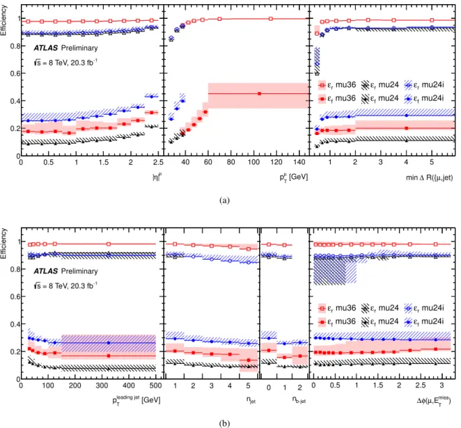
Beside the dependence on the fired trigger described above, the values of

ε_r

and

ε_f

are measured as a function of di

ff

erent variables, including: the lepton

|η|

and p

_T

, the angular distance between the lepton and the closest jet (min

∆

R(`, jet)), the angle in the transverse plane between the lepton and the E

^miss_T

(∆

φ(`,

E

^miss_T

)), the p

_T

of the leading jet, the jet and b-jet multiplicity in the event. Fig.

2

and

3

show

ε_r

and

ε_f

, as a function of the di

ff

erent variables used for the parametrisation. E

ffi

ciencies are shown inclusively for electrons and muons in events with at least one jet and any number of b-jets, but separately for leptons firing each of the triggers, and in the relative lepton p

_T

regions. The significant dependency of the muon real and fake e

ffi

ciencies on the muon p

_T

originates from the isolation requirements imposed to define a tight muon.

These efficiencies are used to compute the weights in Eq.

3

as a function of the different combinations of the variables listed above through:

εk

(x

₁, ...,

x

_N

;

y₁, ..., yM

)

=

1

εk

(x

1, ...,

x

N

)

^M−1 ·

M

Y

j=1

εk

(x

₁, ...,

x

_N

;

yj

). (7) Here the expression

εk

( x

₁, ...,

x

_N

) represents the e

ffi

ciency measured as a function of all the x variables.

The expresssion

εk

(x

1, ...,

x

N

;

yj

) represents instead the efficiency measured as a function of all the x

variables and of the variable

yj

. Equation

7

implies that the full correlation between the variables x (typ-

(9)

[GeV]

miss

ET

0 20 40 60 80 100 120

Events / 5 GeV

0 1000 2000 3000 4000 5000

103

×

ATLAS Preliminary = 8 TeV, 20.3 fb-1

s

1 jets, pretag e + ≥

W

, mT miss

no cuts on ET

loose lepton selection Data 2012

t t Single Top W + jets Z + jets Diboson Uncertainty

(a)

[GeV]

W

mT

0 20 40 60 80 100 120 140 160 180 200

Events / 5 GeV

0 1000 2000 3000 4000 5000

103

×

s

1 jets, pretag e + ≥

W

, mT miss

no cuts on ET

loose lepton selection Data 2012

t t Single Top W + jets Z + jets Diboson Uncertainty

(b)

sig

d0

-20 -15 -10 -5 0 5 10 15 20

Events

10 102

103

104

105

106

107

108

109

1010

1011

1012

1013 ATLAS Preliminary = 8 TeV, 20.3 fb-1

s

1 jets, pretag + ≥

µ

W

, mT miss

no cuts on ET

loose lepton selection

Data 2012 t t Single Top W + jets Z + jets Diboson Uncertainty

(c)

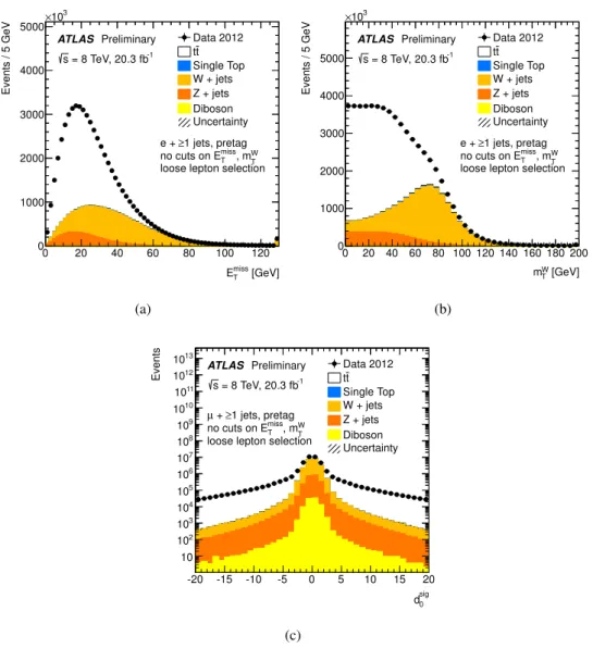
Figure 1: Distributions of the E

^miss_T

(a) and m

^W_T

(b) in e

+

jets events and the transverse impact parameter significance d

₀^sig

(c) in

µ+jets events for data and real lepton expectation from simulated events. Events

are required to have exactly one loose electron or muon and at elast one jet, with no requests on the number of b-tags and no cuts on E

_T^miss

or m

^W_T

. The region between the top of the stacked simulated sources and the data is assumed to come from the non-prompt and fake lepton background contribution.

The only uncertainty shown is the statistical one due to finite Monte Carlo event samples.

ically discrete variables, where no more than three bins are used) and each of the variables

y

(typically continuous variables, with a relatively large number of bins) is taken into account, while the correlation between the

y

variables is neglected. For each of the efficiencies

εk

, only a sub-set of the variables in each category, x or

y, is used, as summarised in Table4. This choice is driven by the observed depen-

dencies, the correlations between the variables and the stability of the estimates. In particular, for each of the efficiencies, the assumption of no correlation between the variables

y

is checked by comparing the observed dependency on the variable

yj

, i.e.

εk

(x

1, ...,

x

N

;

yj

), and the efficiency

εk

(x

1, ...,

x

N

;

y₁, ...yM

) averaged over all the other

{yj⁰}_j⁰_,_j

variables.

The main sources of systematic uncertainties on the non-prompt and fake lepton background deter-

mination with the matrix method originate from the determination of the real efficiency, the use of MC

(10)

e η|

|

0 0.5 1 1.5 2 2.5

Efficiency

0 0.2 0.4 0.6 0.8

s

[GeV]

e

pT

40 60 80 100 120 140

R(e,jet)

∆ min

1 2 3 4 5

r e60

ε ε_r e24vh ε_r e24vhi

f e60

ε ε_f e24vh ε_f e24vhi

(a)

[GeV]

leading jet

pT

0 100 200 300 400 500

Efficiency

0 0.2 0.4 0.6 0.8

s

jet n

1 2 3 4 5

b-jet n

0 1 2

miss) (e,ET

φ

∆

0 0.5 1 1.5 2 2.5 3

r e60

ε ε_r e24vh ε_r e24vhi

f e60

ε ε_f e24vh ε_f e24vhi

(b)

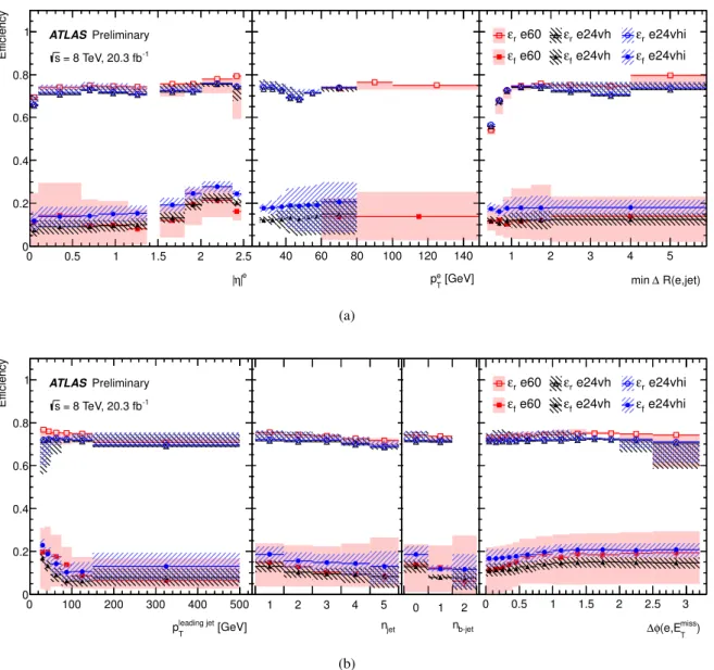
Figure 2: E

ffi

ciencies

ε_r

and

ε_f

for electrons, as measured in data (see text for details), as a function of (from left to right): (a) the electron

|η|

and p

_T

its distance to the closest jet (min

∆

R(e, jet)), (b) the p

_T

of the leading jet, the jet and b-jet multiplicity and the angle in the transverse plane between the electron and the E

_T^miss

(

∆φ(e,

E

^miss_T

)). The e

ffi

ciencies are shown separately for probes which match specifically one of the triggers used to selected data (e24vhi or e60) or the low-p

T

trigger with no isolation requirement (e24vh). The shaded area represents in each bin the combination of the statistical and systematic uncertainties on the e

ffi

ciency measurements. The systematic uncertainties include the e

ff

ect of using the alternative control regions (for both

ε_r

and

ε_f

), and the variations on the amount of real lepton events (for

ε_f

).

simulation to correct the efficiency measurements, differences in the non-prompt and fake background composition in the signal regions and in the regions used to measure the e

ffi

ciencies, and the treatment of the dependence of the e

ffi

ciencies on lepton and event properties.

The uncertainty on the real efficiency measurement method is assessed by measuring the efficiency in

an independent way, by counting the fraction of tight leptons after selecting events with one loose electron

(11)

|µ

|η

0 0.5 1 1.5 2 2.5

Efficiency

0 0.2 0.4 0.6 0.8 1

s

[GeV]

µ

pT

40 60 80 100 120 140

,jet) µ R({

∆ min

1 2 3 4 5

mu36

εr ε_r mu24 ε_r mu24i mu36

εf ε_f mu24 ε_f mu24i

(a)

[GeV]

leading jet

pT

0 100 200 300 400 500

Efficiency

0 0.2 0.4 0.6 0.8 1

s

jet n

1 2 3 4 5

b-jet n

0 1 2

miss) ,ET

µ ( φ

∆

0 0.5 1 1.5 2 2.5 3

mu36

εr ε_r mu24 ε_r mu24i mu36

εf ε_f mu24 ε_f mu24i

(b)

Figure 3: E

ffi

ciencies

ε_r

and

ε_f

for muons, as measured in data (see text for details), as a function of (from left to right): (a) the muon

|η|

and p

_T

its distance to the closest jet (min

∆

R(µ, jet)), (b) the p

_T

of the leading jet, the jet and b-jet multiplicity and the angle in the transverse plane between the muon and the E

_T^miss

(

∆φ(µ,

E

^miss_T

)). The e

ffi

ciencies are shown separately for probes which match specifically one of the triggers used to selected data (mu24i or mu36) or the low- p

_T

trigger with no isolation require- ment (mu24). The shaded area represents the combination in each bin of the statistical and systematic uncertainties on the e

ffi

ciency measurements. The systematic uncertainties include the e

ff

ect of using the alternative control regions (for both

ε_r

and

ε_f

), and the variations on the amount of real lepton events (for

ε_f

).

(muon) in a regions where the contamination from non-prompt and fake lepton events is expected to be

negligible, i.e. by asking E

_T^miss>

150 GeV (m

^W_T >

100 GeV). It is found to be around 7% (between 1 and

5%) in the case of electrons (muons) and to be comparable to the uncertainties on the measurement using

the tag-and-probe method. The latter uncertainties, found to be around 3% for electrons and between

1 and 2% for muons, are dominated by the modeling of the background and the uncertainty on the

(12)

Table 4: Summary of the variables used to parametrise the real and fake lepton efficiencies in the matrix method. The column ‘Trigger’ refers to the specific trigger the lepton matches, p

^lead.jet_T

stays for p

_T

of the leading jet in the event,

∆

R(`, jet) is the angular distance between the lepton and the closest jets,

∆φ(`,

E

^miss_T

) is the angular distance in the transverse plane between the lepton and the missing energy in the event. For each of the efficencies, the variables for which the explicit dependence is used are indicated. The variables are divided in two categories, x and

y, depending the specifc treatment in terms

of correlation. See text for details.

x variables

y

variables

Trigger n

_jet

n

_b−jet |η^`|

p

^`_T

p

^lead.jet_T ∆

R(`, jet)

∆φ(`,

E

^miss_T

)

ε_r

(e)

X X X X X

ε_r

(µ)

X X X X X

ε_f

(e)

X X X X X

ε_f

(µ)

X X X X X

correction based on MC simulation applied in the case of electrons.

The dominant source of systematic uncertainty on the fake efficiency measurement is that originating from the uncertainty on the normalisation of the processes determined from MC simulation in the control regions (mainly Z

+jets and

W

+jets). The uncertainty of their normalisation is∼

30% and corresponds to an uncertainty of 3-13% on the fake efficiency. Another significant source of uncertainty is assessed through the use of alternative control regions to measure the e

ffi

ciencies, defined by di

ff

erent combi- nations of cuts on E

^miss_T

and m

^W_T

, i.e. m

^W_T <

20 GeV for e

+jet,

m

^W_T <

20 GeV and E

^miss_T +

m

^W_T <

60 GeV for

µ+jet events. This approach allows to partially assess the uncertainty coming from the relative

composition of the non-prompt and fake lepton samples in the control and signal regions. Preliminary studies, performed in the case of electrons using simulated events, indicate that this relative composition changes between the control and the single lepton signal regions by the same amount as it does between the default and the alternative control regions. The uncertainty is found to be between 2 and 5%, com- parable to the one found in comparing the fake rates measured in data samples enriched in electrons from conversions, semi-leptonic decays of b

/

c quarks or hadrons (between 5 and 7%). No dedicated systematic uncertainty is applied to the d

^sig₀

extrapolation used for muon

ε_f

: the e

ff

ect of applying or not the correction is already covered by the other systematic uncertainties, in particular the variation on the amount of real lepton events, which modifies significantly the slope of the linear extrapolation, and the use of the alternative CR

_f

, for which no extrapolation is performed.

Finally, di

ff

erent choices for the combinations of variables used in the e

ffi

ciency parametrisation are compared. In particular, the most relevant variations are found to come from the use of min

∆

R(e, jet) instead of

∆φ(e,

E

^miss_T

) in the electron

εf

parametrisation and p

leading jet

T

instead of p

^µ_T

in the muon

εf

one, and are used to assess the uncertainty related to the treatment of the e

ffi

ciency dependencies on lepton and event properties.

To evaluate the uncertainty on the non-prompt and fake and background contribution, the matrix method input e

ffi

ciencies are varied as described above, and the background distributions and yields are then re-derived. The observed deviation of the yields measured where lepton efficiencies are varied is assigned as an uncertainty. The total systematic uncertainty on the estimate is taken as the quadratic sum of the symmetrised individual variations.

In the single-lepton signal regions, this is between 10 and 50%, depending on the channel and on

the jet and b-jet multiplicity. The use of the alternative parametrisation and the real lepton subtraction

from CR

_f

are the dominant sources, with e

ff

ects between 20 and 40% each, in the e

+

jets channel. In

the

µ+jets channel, beside these two sources of uncertainties, with effects between 10 and 25%, the

(13)

Table 5: Summary of the different validation regions used for the matrix method. The term ‘pretag’ is used to indicate that no requirements on the number of b-jets are applied, ‘!tt’ refers to a selection where at least one of the two leptons is not tight, ‘OS’ stays for opposite-sign and ‘SS’ for same-sign charge leptons.

Channel n

_jet/

n

_b−jet

cuts Other cuts e

+

jets

2 jets, pretag

No cuts on E

^miss_T

, m

^W_T

2 jets,

≥

1 b-tags

≥

4 jets, pretag

≥4 jets,≥

1 b-tags

µ+

jets

2 jets, pretag

No cuts on E

^miss_T

, m

^W_T

2 jets,

≥

1 b-tags

≥

4 jets, pretag

≥4 jets,≥

1 b-tags eµ

≥2 jets, pretag

SS, H

_T >

100 GeV

≥2 jets,≥

1 b-tags

≥2 jets, pretag

OS, !tt, H

_T >

100 GeV

≥2 jets,≥

1 b-tags

alternative estimate for

ε_r

produces a relatively large deviation, around 15%.

6.3 Results in lepton + jets validation regions as obtained using the matrix method The background predictions are compared to data in validation regions, summarised in Table

5. In the

lepton

+

jets channels, these regions are defined as the signal regions but without applying the E

_T^miss

and m

^W_T

cuts. These regions include the control regions where the fake efficiencies are measured and are therefore used to carry out a consistency check of the method.

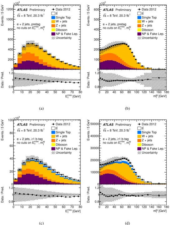
Fig.

4

shows the distributions of E

_T^miss

and m

^W_T

in the e

+

jets validation regions with two jets. Distribu-

tions show the non-prompt and fake lepton background estimates together with the real lepton predictions

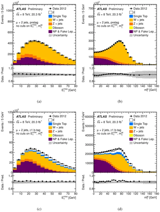
from MC simulation and compared with data. Similarly, Fig.

5

shows the same distributions for

µ+jets

events. In Appendix

B

results in regions with four or more jets are shown. The agreement between data

and prediction is within the uncertainty of the non-prompt and fake background in regions of phase space

where this background dominates. In regions where it is negligible, data and prediction agree within the

uncertainties on the MC-derived processes based on Ref. [56]. Note that the uncertainty band shown in

the Figures does not contain the uncertainty on the MC-derived backgrounds.

(14)

Events / 5 GeV

0 200 400 600 800 1000 1200

103

×

s

e + 2 jets, pretag

W

, mT miss

no cuts on ET

Data 2012 t t Single Top W + jets Z + jets Diboson NP & Fake Lep.

Uncertainty

[GeV]

miss

ET

0 10 20 30 40 50 60 70 80

Data / Pred. 0.8

1 1.2

(a)

Events / 5 GeV

0 100 200 300 400 500 600

103

×

s

e + 2 jets, pretag

W

, mT miss

no cuts on ET

Uncertainty

[GeV]

WT

m 0 20 40 60 80 100 120 140 160 180

Data / Pred. 0.8

1 1.2

(b)

Events / 5 GeV

0 20 40 60 80 100

103

×

s

1 b-tag e + 2 jets, ≥

W

, mT miss

no cuts on ET

Uncertainty

[GeV]

miss

ET

0 10 20 30 40 50 60 70 80

Data / Pred. 0.8

1 1.2

(c)

Events / 5 GeV

0 10000 20000 30000 40000

s

1 b-tag e + 2 jets, ≥

W

, mT miss

no cuts on ET

Uncertainty

[GeV]

W

mT

0 20 40 60 80 100 120 140 160 180

Data / Pred. 0.8

1 1.2

(d)

Figure 4: Distributions of E

_T^miss

(a, c) and m

^W_T

(b, d) in e

+

jets events with exactly two jets before (a, b) and after (c, d) requiring at least one b-jet, without any cuts on E

^miss_T

and m

^W_T

. The data is compared to the real lepton expectation from simulation, showing separately the contributions from t¯ t, single top, W

+jets,

Z

+

jets and dibosons normalised to their cross-sections, and non-prompt and fake lepton backgrounds (referred to as ‘NP & Fake Lep.’) estimated with the matrix method. The shaded area represents the combination of the statistical and the systematic uncertainties on the matrix method estimate in each bin.

The systematic uncertainties on the processes predicted by the MC simulation are not shown.

(15)

Events / 5 GeV

0 200 400 600 800 1000

103

×

s

+ 2 jets, pretag µ

W

, mT miss

no cuts on ET

Uncertainty

[GeV]

miss

ET

0 10 20 30 40 50 60 70 80

Data / Pred. 0.8

1 1.2

(a)

Events / 5 GeV

0 100 200 300 400 500 600 700

103

×

s

+ 2 jets, pretag µ

W

, mT miss

no cuts on ET

Uncertainty

[GeV]

WT

m 0 20 40 60 80 100 120 140 160 180

Data / Pred. 0.8

1 1.2

(b)

Events / 5 GeV

0 20 40 60 80 100 120

103

×

s

1 b-tag + 2 jets, ≥ µ

W

, mT miss

no cuts on ET

Uncertainty

[GeV]

miss

ET

0 10 20 30 40 50 60 70 80

Data / Pred. 0.8

1 1.2

(c)

Events / 5 GeV

0 10000 20000 30000 40000 50000

s

1 b-tag + 2 jets, ≥ µ

W

, mT miss

no cuts on ET

Uncertainty

[GeV]

W

mT

0 20 40 60 80 100 120 140 160 180

Data / Pred. 0.8

1 1.2

(d)

Figure 5: Distributions of E

^miss_T

(a, c) and m

^W_T

(b, d) in

µ+

jets events with exactly two jets before (a, b) and after (c, d) requiring at least one b-jet, without any cuts on E

^miss_T

and m

^W_T

. The data is compared to the real lepton expectation from simulation, showing separately the contributions from t¯ t, single top, W

+jets,

Z

+

jets and dibosons normalised to their cross-sections, and non-prompt and fake lepton backgrounds (referred to as ‘NP & Fake Lep.’) estimated with the matrix method. The shaded area represents the combination of the statistical and the systematic uncertainties on the matrix method estimate in each bin.