Momentum resolution of a tracking detector
Data analysis 2021 – Group project V
Vadym Denysenko, Patrick Owen, Olaf Steinkamp April 13, 2021
1 Motivation
In this project, you are going to simulate a simple particle tracking detector for the reconstruction of the trajectories of charged particles. One goal in the reconstruction of such trajectories is to estimate the position at which the particle was created, the second goal is to measure its momentum.
To measure the momentum, a magnetic field is applied. The magnetic field exerts a Lorentz force on moving charged particle. If the field is homogeneous, the particle is forced onto a circular trajectory with radius of curvature
ρ = pT q·B
whereBis the strength of the magnetic field,qis the charge of the particle, andpTis the component of its momentum transverse to the magnetic field lines. Expressing ρ in metres, B in T and q in units of the elementary charge, the transverse momentum in GeV is
pT ≈ 0.3·e·B·ρ .
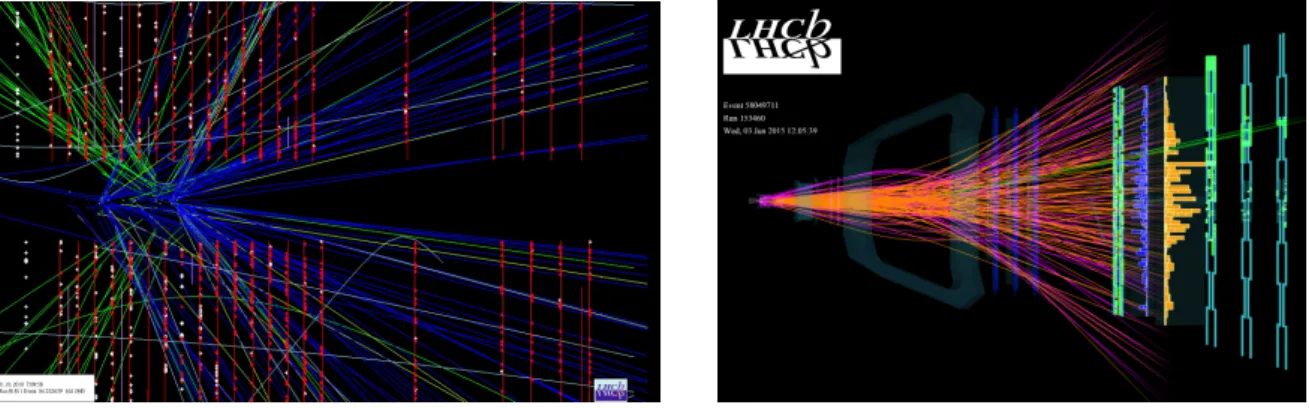
For illustration, Fig. 1 shows an “event display” from the LHCb experiment at CERN. You are going to estimate the spatial resolution and the momentum resolution for a similar but simplified detector setup.
An important cross check in simulation studies is the so-called “pull”, defined as pull = reconstructed quantity−generated quantity
uncertainty on reconstructed quantity ,
where the “uncertainty on reconstructed quantity” is for example that returned from your fit to the data. If the reconstruction is unbiased and the uncertainties on the reconstructed quantities is estimated correctly, the distribution of the pulls over many simulated experiments should follow a Gaussian distribution withµ= 0 andσ = 1. Ifµdeviates significantly from zero, the measurement is biased. Ifσ deviates significantly from one, the uncertainties are not estimated correctly.
2 Setup
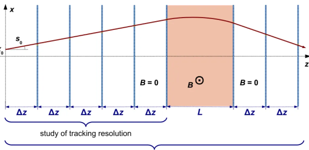
The detector setup is illustrated in Fig. 2. It consists of n detection planes that measure the x coordinate of the trajectory and are spaced at equal intervals ∆z along the z axis, followed by a
Figure 1: Two events displays from the LHCb experiment at CERN. The display on the left shows a close-up of the “interaction region” where protons from the two beams circulating in the LHC are brought into collisions. The detection planes of the tracking detector are illustrated by thin, red vertical lines, hits in these detection layers are illustrated by little red rectangles. Blue, green and yellow lines indicate reconstructed trajectories. There are two regions in which lots of trajectories seem to intersect, indicating that in this event two proton-proton collisions seem to have occured. The display on the right shows reconstructed trajectories of charged particles as they traverse the full detector from left to right. The trajectories are bent by the field of the LHCb dipole magnet. Positively and negatively charged particles are bent in opposite directions and low-momentum particles are bent more than high-momentum particles.
magnet with lengthL and field lines orthogonal to thez and x axes, and another three detection planes spaced at equal intervals ∆z.
Each detection plane consists of 500µm wide cells that give a signal when a particle passes through the cell. The detector does not provide position resolution within the cell, i.e. for the reconstruction of the trajectory you have to use the position of the cell that was hit.
The field is constant (homogeneous) inside the magnet and zero outside the magnet. This means particles follow a straight trajectory before and after the magnet and a circular trajectory inside the magnet.
3 Tracking resolution
In this first part of your study you make use only of the firstndetection planes before the magnet.
To start with, setn= 5 and ∆z= 2 cm.
As a warm-up exercise, generate a single particle trajectory starting at z0 = 0 and x0 =xtrue0 and propagating towards positivezwith a small slopes0. Drawxtrue0 from a Gaussian distribution with mean 0 and standard deviation 1 mm and draw strue0 from a Gaussian distribution with mean 0 and standard deviation 0.1 rad.
(a) Generate a detector response (a hit) at each intersection with a detection layer, i.e. calculate thexposition of the trajectory at the z position of the detection layer, determine which cell was hit and store the position of this cell as the position of the hit in this layer.
(b) Discuss and decide how you want to model the uncertainty on the measured hit positions.
Use this uncertainty model, fit a straight line to the reconstructed hit positions from all n detection layers, and determine the reconstructed slopesreco0 and impact parameterxreco0 with their uncertainties.
2
z
Δz x
Δz Δz Δz Δz
x0 s0
B = 0
Δz Δz B = 0 B
L
⊙
study of tracking resolution
study of momentum resolution
Figure 2: Illustration of the setup.
(c) Draw the generated trajectory as a dashed line, the calculated hit positions with their assigned uncertainty as points with errorbars, and the reconstructed trajectory as a full line.
To estimate the resolution of your detector in x0 and s0, generate 1’000 trajectories with z0 = 0, xtrue0 Gaussian distributed with mean 0 and standard deviation 1 mm andstrue0 Gaussian distributed with mean 0 and standard deviation 0.1 rad.
(d) For each of the 1’000 trajectories, generate hit positions in thendetection layers and deter- minesreco0 and xreco0 with their uncertainties as you did in the warm-up exercise.
(e) Generate histograms of the residual distributions, sreco0 −strue0 and xreco0 −xtrue0 . Determine the mean and standard deviation for each of the two distributions.
(f) Calculate and histogram the pulls for sreco0 and xreco0 . Determine the means and standard deviations of the two pull distributions.
4 Momentum resolution
For this second part of your study you make use of the full setup, including the magnet and the three detection layers behind the magnet. Setn= 5, ∆z= 2 cm, L= 10 cm and B= 0.5 T.
As a warm-up exercise, generate a single particle trajectory for a particle with pT = 0.3 GeV, xtrue0 drawn from a Gaussian distribution with mean 0 and standard deviation 1 mm and withstrue0 drawn from a Gaussian distribution with mean 0 and standard deviation 0.1 rad. Randomly assign chargeq = +1 orq =−1 to the particle.
(a) Extrapolate the trajectory to the z positions of the eight detection layers (five before and three after the magnet). Generate hit positions as you did in Sec.3. Draw the trajectory and the hit positions with their uncertainties.
(b) Fit straight lines to the hits in the stations before and after the magnet and determineprecoT and its uncertainty from the angle between these two lines (see Appendix).
To estimate the momentum resolution of your detector, generate 1’000 trajectories withxtrue0 Gaus- sian distributed with mean 0 and standard deviation 1 mm and with strue0 Gaussian distributed with mean 0 and standard deviation 0.1 rad. Randomly assign charge q = +1 orq = −1 to each
3
particle.
(c) For each of the 1’000 trajectories, generate hit positions in the detection layers and determine precoT with its uncertainty as you did in the warm-up exercise.
(d) Fill a histogram with precoT −ptrueT . Determine the mean and the standard deviation of the distribution.
(e) Calculate and histogram the pulls for precoT . Determine the mean and the standard deviation of the pull distribution.
Repeat the exercise forptrueT = 0.1,1,2,5,10,20 GeV/c. Observe how the resolution onpT changes as a function ofptrueT .
Repeat the exercise forptrueT = 0.3 GeV and B= 1.0,1.5,2.0 T. Observe how the resolution onpT changes as a function ofB.
Appendix
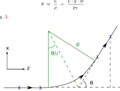
Assuming the bending radius of the particle trajectory is much larger than the length of the magnetic field, thepT of the particle can be estimated from the bending angle
θ ≈ L
ρ = L·q·B pT
as illustrated in Fig. 3.
Figure 3: Reconstructing thepT of the particle from the bending angle θ in its trajectory.
4