Studies of Direct Stau Production with the ATLAS Detector at the LHC at 13 TeV

(1)

Studies of Direct Stau Production with the ATLAS Detector at the LHC at 13 TeV

P

ATRICK

S

ELLE

Master Thesis

(2)

(3)

Technical University of Munich Boltzmannstraße 15

Physics Department

The Max Planck Institute for Physics Föhringer Ring 6

Master Thesis

Studies of Direct Stau Production with the AT- LAS Detector at the LHC at 13 TeV

Patrick Selle

Abgabetermin:

test2. Mai 2019 Prüfer:

testProf. Dr. rer. Hubert Kroha

Ehrenwörtliche Erklärung

Ich erkläre hiermit ehrenwörtlich, dass ich die vorliegende Arbeit selbstständig und ohne Benutzung anderer als der angegebenen Hilfsmittel angefertigt habe; die aus fremden Quellen (einschließlich elektronischer Quellen) direkt oder indirekt übernommenen Gedanken sind ausnahmslos als solche kenntlich gemacht.

Munich, 2. Mai 2019

Patrick Selle

(4)

(5)

Studies of Direct Stau Production with the ATLAS Detector at the LHC at 13 TeV

Patrick Selle

(6)

(7)

Abstract

Supersymmetry (SUSY) provides solutions to many open problems of the Standard Model (SM) such as the hierarchy problem and the mystery of Dark Matter (DM). In some SUSY models, the supersymmetric partner of theτ-lepton, the stau ( ˜τ), is predicted to be lighter than the other sleptons with a mass near the electroweak scale. Models involving co-annihilation between the stau and the lightest supersymmetric particle (LSP), which can be almost degenerate in mass, reproduce the observed relic DM density of the universe. At the LHC, staus would be pair-produced and decay into their SM counterpart and the LSP. Typical stau events would, therefore, be characterized by the presence of two SMτ-leptons and large missing energy arising from the LSP pair and the neutrinos from the tau decays. This thesis presents the search strategy for direct stau pair production with the ATLAS detector at the LHC at a center-of-mass energy of 13 TeV. The focus of the study is on final states with one hadronically and one leptonically decayingτ-lepton. The selection of signal regions is optimized to achieve the highest possible signal sensitivity using simulated data in the ATLAS detector. Stau-LSP mass regions between 170 and 270 TeV and 1 and 55 TeV, respectively, can be exluded at 95 % CL.

(8)

(9)

It is the task of science to decipher the mysteries of nature. Today we believe that matter is composed of indivisible point-like constituents, the elementary particles. The first of these fundamental particles, the electron, was discovered in 1897 by Sir Joseph John Thomson [1]. Since the discovery of the electron more elementary particles have been found. The Standard Model (SM) of particle physics, a quantum field theory describing the known particles and their interactions was established in the last century. The verification of its particle content was completed with the discovery of the Higgs boson at the Large Hadron Collider in 2012 [2]. The SM describes three of the four fundamental forces, the electromagnetic, the weak and the strong force. Only gravity has so far resisted all attempts to formulate it in the framework of a quantum field theory and, therefore, is not part of the SM.

All predictions of the SM so far are in excellent agreement with experiments, but there are many open questions. Most prominently, Dark Matter (DM) is not described by the SM. Based on astrophysical and cosmological observations due to emission of electromagnetic radiation, we know that there must be more gravitational matter than can be observed. This invisible matter is called Dark Matter.

The origin and composition of Dark Matter is still unknown. Another open question in the SM is caused by the huge difference between the electroweak and the gravitational mass scales which leads to the fine-tuning problem of the mass of the Higgs boson at the electroweak scale. These open questions suggest that a new, more fundamental theory must exist. One possible extension of the SM which allows to explaining many questions is supersymmetry (SUSY), which assigns a superpartner to each particle of the SM and thus doubles the number of elementary particles. At the Large Hadron Collider (LHC) at CERN, extensive searches for supersymmetric particles have been performed, but nothing has been found yet. One difficulty is due to the many free parameters of supersymmetric extensions of the SM and the associated diversity of production and decay modes.

One attractive channel to search for supersymmetry which has not been strongly constrained yet at the LHC is direct stau pair production. In this thesis this channel has been investigated using

(12)

1 Introduction

simulated data of the ATLAS detector from Run 2 of the LHC between the years of 2015 and 2018 at a center-of-mass energy of

√s =13 TeV. In Chapter 3 the experimental setup of the ATLAS detector and the particle identification algorithms used in the experiment are briefly described. Chapter 4 describes the current status of the search for direct stau pair production together with the object and event selection. Chapter 5 discusses the Monte Carlo simulations used for the analysis. Finally, in Chapter 6 the optimization of the signal region using one lepton and one hadronicτ-lepton is presented.

The results of the studies are summarized in Chapter 7.

(13)

CHAPTER TWO

THE THEORETICAL OVERWIEV

That I recognize what holds the world together.

Johann W. v. Goethe

These words of Goethe match the mission of particle physics very well. Particle physics attemps to understand the structure of the universe and which forces hold it together. Particle accelerators and detectors are built to explore the fundamental laws of nature and the properties of matter. The Standard Model of particle physics (SM) summarizes all present knowledge of visible matter.

The SM is a quantum field theory based on a spontaneously broken localSU(3)C×SU(2)L×U(1)Y

gauge symmetry. The particle content of the SM and the interactions governed by the local gauge symmetries are introduced in Section 2.1 together with the successes and limitations of the theory.

The principles of SUSY and the Minimal Supersymmetric extension of the Standard Model (MSSM) are discussed in Section 2.2.

2.1 The Standard Model of Particle Physics

The SM of particle physics describes all known particles and three of the four fundamental forces, the electromagnetic, the strong and the weak interactions. It is a gauge invariant quantum field theory based on the symmetry groupSU(3)_C×SU(2)_L ×U(1)_Y[3–6].

There are three types of fundamental particles according to their spin s, fermions with s = ¹₂, gauge bosons withs =1 and the Higgs boson withs =0. For each particle there is an antiparticle with the same mass but opposite electric charge. The fermions can be subdivided into leptons and quarks which appear in three generations. Each generation contains one charged lepton, one neutral

(14)

2 The Theoretical Overwiev

neutrino and two quarks. Corresponding particles of the different generations have the same quantum numbers but differ in mass.

Quarks interact via the strong, the electromagnetic and the weak interaction. Quarks carry a color quantum number which can take three different values, denoted by red, green and blue. The quarks form colorless bound states consisting of either three quarks, the baryons, or of a quark and an antiquark, the mesons. The leptons interact via the weak interaction and in the case of charged leptons also via the electromagnetic interaction.

Fermions are described by Dirac spinors ψ_D, which are solutions of the Dirac equation. The fermions are arranged in left-handed lepton and quark doublets

L_L =* ,

ν_e e+

-L

,* ,

νµ

µ+ -L

,* ,

ντ

τ+ -L

, Q_L =*

, u d+

-L

,* , c s+

-L

,* , t b+

-L

, (2.1)

and in right-handed lepton and quark singlets

`R= e_R, µR, τR u_R =u_R, c_R, t_R d_R =d_R, s_R, b_R (2.2) of the weak gauge groupSU(2)L, a manifestation of maximum parity violation by the weak interaction.

The interactions are introduced by requiring invariance of the equations of motion under local gauge transformations [7]

φ(x) →eîαâ^(x)Tâφ(x), (2.3)

whereα^aare the phase parameters andT_athe generators of the corresponding Lie group. In order to achieve invariance under local gauge transformations, a gauge boson field with specific coupling and transformation properties has to be introduced for each generator of the gauge groups. The strong interaction is described by the SU(3)C gauge group associated with eight massless gluons fields mediating the interaction and the gauge coupling constantα_s. The electroweak interaction is described by aSU(2)L×U(1)Y gauge group with three gauge bosonsWⁱ(i=1,2,3) with weakSU(2)L isospin chargesT_i = (T₁,T₂,T₃)and coupling strengthgW and a gauge bosonBassociated withU(1)Yweak hypercharge and coupling constantg_Y. The hyperchargeY is related to the third component of the weak isospinT₃and the electric chargeQby

Q=T₃+Y 2

. (2.4)

(15)

2.1 The Standard Model of Particle Physics

The two fieldsW¹andW²mix to form the charged weak gauge boson mass eigenstatesW^±: W^±= 1

√ 2

W¹∓iW²

. (2.5)

TheW³andBfields mix resulting in the photon fieldAand the weak neutral gauge bosonZ as mass eigenstates:

* , Z A+

-

=* ,

cosθ_W sinθ_W

−sinθ_W cosθ_W+ -

* ,

W³ B +

-

, (2.6)

whereθ_W is the Weinberg angle given by tanθ_W = _g^g_W^Y .

The local gauge invariance requires the gauge bosons to be massless. However, the measured masses of the Z andW^±bosons discovered early in 1983 are massive with m_W = 80.4 GeV and m_Z = 91.2 GeV, respectively [8, 9]. In 1964, Peter Higgs, Francois Englert and Robert Brout introduced the so-called Higgs mechanism based on spontaneous electroweak gauge symmetry breaking [10,11]. For this purpose a complex scalar weak isospin doublet field

Φ=* ,

φ⁺ φ⁰+

-

(2.7) with four degrees of freedom with potential

V(|Φ|)= µ²|Φ|²+λ|Φ|⁴ (2.8)

is introduced, where λ is a dimensionless self-coupling constant and µthe mass parameter. For λ > 0 and µ² < 0 this results in a non-zero vacuum expectation valueυ = √

2|Φ₀| = q

−µ² λ . A particular choice of the vacuum state, e.g. hΦi= ^√¹

2

* , 0 υ+

-

, breaks theU(1)Y×SU(2)Lgauge symmetry spontaneously. Eliminating by gauge transformation the phase correspodning to the broken symmetries connecting different ground states leads to mass terms for theW^±and theZ bosons, while the photon remains massless. The Higgs boson is the massive excitation of the scalar field from the ground state.

The quarks and charged leptons acquire masses via Yukawa coupling to the Higgs field. The Higgs boson was discovered in 2012 by the ATLAS and CMS experiments at the LHC with a mass of about 125 GeV [12]. In 2013 the Nobel Prize in physics was awarded jointly to Francois Englert and Peter W. Higgs for the introduction of the Higgs mechanism and the prediction of the Higgs boson.

(16)

2.1.1 Successes and limitations of the Standard Model

The SM has successfully passed all experimental tests so far. However, there are several questions that cannot be explained by the SM.

First of all, the SM does not describe (quantum) gravity [13]. Furthermore in the SM, the neutrinos are assumed to be massless. The observation of neutrino oscillations however, means that they must have mass [14]. The rotation curves of galaxies cannot be explained by the amount of visible, baryonic matter described by the SM as well as several other astrophysical observations which require the introduction of Dark Matter, which only interacts weakly or even only gravitationally with the SM particles [15].

Dark energy has been postulated to explain the accelerated expansion of the universe [16]. From astrophysical and cosmological observations it is dervived that only 4.9 % of the energy content of the universe is SM matter, whereas 26.8 % is Dark Matter and the remaining fraction Dark Energy, neither of which is described by the SM. Also the asymmetry between matter and antimatter in the universe cannot be explained by the observed CP violation by the weak interaction which is described by the SM.

Another problem, one of the key arguments for supersymmetry, is the so-called hierarchy-problem.

Figure 2.1: Leading-order Feynman diagrams of the quantum corrections to the Higgs boson propagator for a fermion (a) or a scalar boson (b) coupling to the Higgs boson [17].

The mass of the Higgs boson receives loop corrections from every particle coupling to the Higgs field (see Figure 2.1). The leading-order correction due to the coupling to a fermion f is given by:

∆m²_H,_f =−|λ_f|²

8π² Λ², (2.9)

(17)

2.2 Supersymmetry while it is:

∆m²_H = + λs

16π²

fΛ²−2m²_sln(Λ/ms)...g

(2.10) for coupling to a scalar boson, whereΛis the cut-off energy up to which the SM is valid, andm_s andλ_s the scalar mass and coupling, respectively. If there is no new physics up to the Planck scale where effects of the quantum gravity can no longer be neglected, the cut-off energy is near the Planck massm_P ≈ 10¹⁸GeV. To stabilize the Higgs mass at its measured valuem_H = 125 GeV near the electroweak scale against the quadratic corrections inΛ, unnatural fine-tuning of the SM parameters is required. Here, SUSY provides an elegant solution cancelling the quadratic divergences in the Higgs mass radiative corrections.

2.2 Supersymmetry

Supersymmetry (SUSY) [17] is a symmetry between fermions and bosons and currently most favoured and complete extension of the SM. Supersymmetry requires invariance and transformations with an anti-commuting spinor operator ˆQwith the property,

Qˆ |Bosoni= |Fermioni, Qˆ |Fermioni=|Bosoni. (2.11) Assuming this invariance requires the introduction of superpartners to each particle of the SM which must be heavier than the SM particles because they otherwise have been discovered. They have the same quantum numbers as their SM counter parts with the exception of the spin which differs by ¹₂~. In other words, each SM fermion gets assigned a bosonic partner and vice versa.

All fields of the SM and their SUSY partners form irreducible representations of the supersymmetry algebra, the supermultiplets described by superfields. The Higgs mass corrections due to the superpartners have opposite sign and cancel each other to first order, solving the fine-tuning problem.

SUSY has to be a broken symmetry, since the superpartners of the SM particles have to be much heavier. There are several ways to break SUSY which lead to additional mass terms on the order ofm_soft. Leaving non-vanishing correction terms to the Higgs boson mass of the form

∆m²_H =m²

soft

" λ_s 16π²ln

Λ m_soft +...

#

, (2.12)

whereλis a dimensionless coupling. In order to solve the fine-tuning problem, the SUSY breaking scale, therefore, must not be higher than a few TeV [18]. Supersymmetric particles therefore should be produced in thepp-collisions at the LHC.

(18)

Table 2.1: The gauge supermultiplets consinsts of the eight color superfieldsV^α, the triplet weak superfieldsVⁱ and the hypercharge singletV

Superfield SU(3)C ×SU(2)L ×U(1)Y spin−1 spin−1/2 Names

V^α (8,1,0) g_α Hg_α gluons, gluinos ,(α=1, ...,8)

Vⁱ (1,3,0) Wⁱ WHⁱ W bosons, winos,(i=1,2,3)

V (1,1,0) B⁰ BH⁰ Bboson, bino

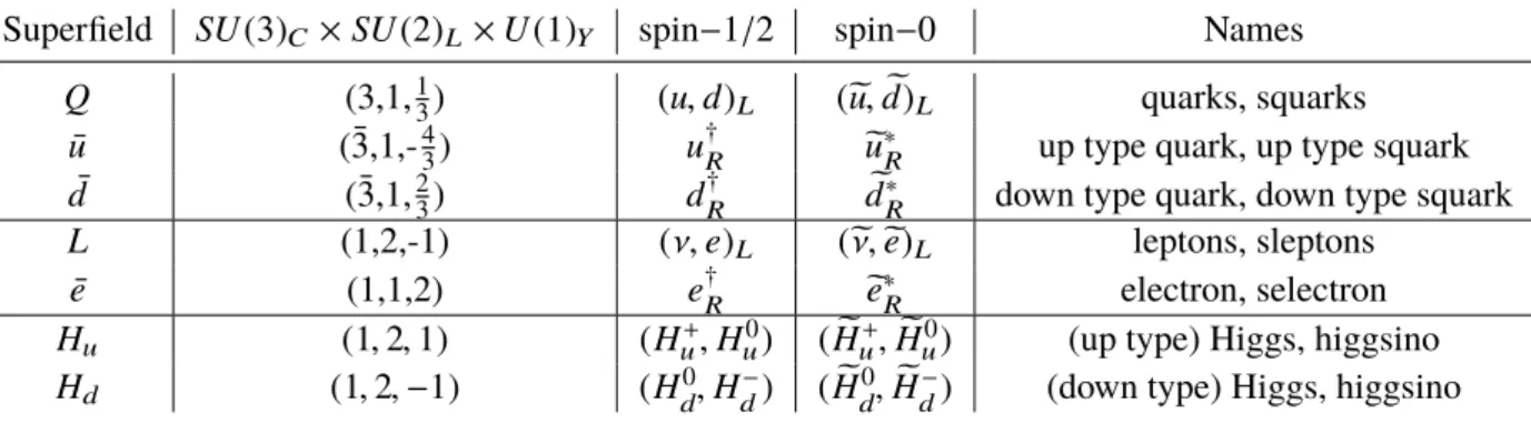
Table 2.2: The chiral supermultiplets consinsts of the superfields corresponding to the fermions and the two complex Higgs doublets

Superfield SU(3)C ×SU(2)L ×U(1)Y spin−1/2 spin−0 Names

Q (3,1,¹₃) (u,d)L (Hu,d)HL quarks, squarks

u¯ ( ¯3,1,-⁴₃) u^†_R Hu^∗_R up type quark, up type squark d¯ ( ¯3,1,²₃) d^†_R dH^∗_R down type quark, down type squark

L (1,2,-1) (ν,e)_L (Hν,He)_L leptons, sleptons

e¯ (1,1,2) e^†_R He^∗_R electron, selectron

H_u (1,2,1) (H_u⁺,H_u⁰) (HH_u⁺,HH_u⁰) (up type) Higgs, higgsino H_d (1,2,−1) (H_d⁰,H_d⁻) (HH_d⁰,HH_d⁻) (down type) Higgs, higgsino

2.2.1 The Minimal Supersymmetric Standard Model

The Minimal Supersymmetric extension of the Standard Model (MSSM) contains the minimum number of additional particles required to extend the SM to a supersymmetric theory [19]. Since the MSSM is based on the same gauge group as the SM, there are 8 colored vector superfieldsV^α, 3 weak superfieldsVⁱand a hypercharge singletV as shown in Table 2.1. The superfields corresponding to the quarks and leptons are shown in Table 2.2. The spin-0 partners of the leptons and quarks are called sleptonsH`and squarksHq, respectively. The spin−¹

2 partners of the gauge bosons are called gauginos.

In order to avoid gauge anomalies, separate Higgs doublets coupling to up- and down-type fermions are needed, resulting in five physical Higgs bosons after electroweak symmetry breaking:

• two neutral scalar particlesh⁰,H⁰, whereh⁰has properties of the SM Higgs boson,

• two electrically charged particlesH^±,

• and a neutral pseudoscalar particleA⁰.

(19)

2.2 Supersymmetry The supersymmetric partners of the Higgs bosons, the so called higgsinos, mix with the electroweak gauginos resulting in four neutralinos Hχ⁰_i (i=1,2,3,4) and four charginos Hχ^±_i (i=1,2). The whole particle content of the MSSM is summarized in Figure 2.2.

Figure 2.2: Particle content of the Minimal Supersymmetric Standard Model [20].

(20)

(21)

CHAPTER THREE

THE ATLAS EXPERIMENT

3.1 The Large Hadron Collider

Figure 3.1: The Cern accelerator complex [21].

The LHC at CERN, the European centre for particle physics near Geneva, is a circular storage ring colliding protons at a centre-of-mass energy of

√s = 13 TeV and an instantaneous luminosity of

(22)

3 The ATLAS Experiment

L=1.5×10³⁴cm⁻³s⁻¹[22]. It is located in a tunnel at a depth of 50 m to 175 m underground and has a circumference of 26.6 km. The LHC utilizes 1232 superconducting dipole magnets to keep the protons on their circular path. They are operated at a maximum current of 12 kA resulting in a magnetic field of 8.3 T. The proton beams consist of 2808 bunches of 10¹¹protons each. The bunch spacing time is 25 ns.

Before injection into the LHC, the protons are pre-accelerated in several other accelerators, first a linear accelerator, then the Proton Synchrotron (PS) and, finally, the Super Proton Synchrotron (SPS), which increases the proton energy to the injection energy of 450 GeV. Figure 3.1 schematically illustrates the CERN accelerator complex. The protons collide at four interaction points, where the main experiments, ATLAS, CMS, LHCb and ALICE, are located. ATLAS and CMS are general purpose experiments, designed for precision tests of the SM and for the search for new physics and, in particular, for the discovery of the Higgs boson. LHCb studies B-hadron decays and CP violation while ALICE is designed to investigate the properties of the quark-gluon plasma in heavy ion collisions.

3.1.1 Luminosity and Pile-up

The number of collision eventsN_expfor a given process is given by N_exp=σ·L =σ·

Z

Ldt, (3.1)

where σ is the production cross-section of the process, L the integrated luminosity and L the instantaneous luminosity. The instantaneous luminosity depends on number of bunches per beamn_b, the number of particles in each bunchN_p, the revolution frequency f and the spread of the beam in each directionσi (i= x,y):

L= n_bN_p²f 4πσxσy

. (3.2)

The data taking from 2015 to 2018 is called Run 2. Figure 3.2 shows the total delivered integrated luminosity by the LHC (green), the recorded integrated luminosity by the ATLAS detector (yellow) and data which can be used for physics (blue). To reach such high luminosities the beams have to be highly focused. This leads to multiple ppinteractions per bunch collision, an effect called pile-up.

The average number of additional interactions per bunch crossing is shown in figure 3.3.

(23)

3.2 The ATLAS Detector

Figure 3.2: Total Integrated Luminosity and Data Quality in 2015-2018 [23].

Figure 3.3: Luminosity-weighted distribution of the mean number of interactions per bunch crossing for the 2015-2018 collision data. [24].

Figure 3.4: Schematic view of the ATLAS detector [25].

3.2 The ATLAS Detector

The ATLAS (A Toroidal LHC ApparatuS) is one of the two multi-purpose detectors hosted at the LHC, shown in Figure 3.4. It is the largest of the experiments, with a length of 44 m, a diameter of 25 m and a mass of about 7000 tons. The ATLAS physics program covers the search for new particles like the Higgs boson or dark matter, the presicion measurement of SM processes as well as the investigation of CP violation in b-hadron decays. In the central barrel region, the detector components are arranged in cylindrical layers around the beam pipe. In the endcap regions the components are mounted on disks perpendicular to the beam.

(24)

3.2.1 ATLAS Coordinate System

ATLAS uses a right-handed coordinate system of which the origin cuts the nominal interaction point.

Thez-axis is the proton beam axis, whereas thex-axis points towards the centre of the LHC ring. The x-y-plane is the transverse plane with respect to the proton beam. To describe points in the detector, spherical coordinates(r, θ, φ)are used, wherer is the distance from the origin,θ the polar angle and φthe azimuthal angle in thex-y-plane. Instead of the polar angle the pseudorapidity

η=−ln

"

tanθ 2

#

(3.3)

is used. The transverse momentum of a particle relative to the beam axis is defined asp_T =q

p²_x+p²_y =

|p|/coshη and the corresponding transverse energy, E_T, is defined as E_T = E/coshη. Angular distances are defined as∆R=p

∆η²+∆φ².

3.2.2 The Inner Detector

Figure 3.5: Cut-away view of the ATLAS Inner De- tector [25]

.

Figure 3.6: Barrel region pf the ATLAS Inner Detector [25]

The innermost part of the ATLAS detector is a highly granular tracking system called the Inner Detector (ID) [26]. The ID surrounds the collision point and consists of a silicon pixel detector, the Semiconductor Tracker (SCT) consisting of silicon microstrip detectors and the Transition Radiation Tracker (TRT) which are immersed in a 2 T solenoidal magnetic field. The layout of the ID with its tree sub-systems is illustrated in Figure 3.5 and Figure 3.6. The ID measures the trajectories of charged particles within|η| <2.5. The track curvature is used to determine the charge and the momentum of

(25)

3.2 The ATLAS Detector the particle. The track measuring also allows for the reconstruction of the primary interaction vertex and of secondary decay vertices.

The Pixel Detector is the innermost part of the ID. It consists of silicon pixel sensors with high granularity that are arranged in three cylindrical layers around the beam pipe and in three discs in each endcap region. The resolution of the Pixel Detector is 10 µm in the transverse plane and 115 µm in beam direction. A new innermost layer, the so called Insertable B-Layer (IBL), was added during the long shutdown 2013-2014. The IBL improves the reconstruction of secondary vertices used for the identification ofτleptons and b-jets.

The Semiconductor Tracker (SCT) surrounds the Pixel Detector. It consists of four cylindrical layers and nine discs in each endcap. It is made of silicon microstrip sensors. The spatial resolution is 17 µm in theR−φplane and 580 µm inz-direction.

The Transition Radiation Tracker (TRT) is the outermost part of the ID. It covers a pseudorapidity region of|η| <2. It consists of up to 73 layers of straw drift tubes with a diameter of 4 mm for charged particle track reconstruction. The tubes are filled with a gas mixture of 70 % Xe, 27 % CO2 and 3 % O2. Charged particles, especially electrons passing the radiator foils between the straws emit transition radiation photons, which are detected by the straw tubes and used for electron identification.

3.2.3 The Calorimeter

The Calorimeter System surrounds the Inner Detector and measures the energy of particles interacting electromagnetically or hadronically [25]. There are two main parts: the electromagnetic calorimeter and the hadronic calorimeter. Both consist of metal absorber plates interleaved between active detector material, liquid argon in the electromagnetic and hadronic endcap calorimeters and scintillating plastic tiles in the barrel hadronic calorimeter. The whole calorimeter system covers a pseudorapidity range of

|η| <4.9 and the whole azimuthal angle range. An overview of the different calorimeter sub-systems is given in Figure 3.7.

The electromagnetic calorimeter (ECAL), consisting of a barrel and an endcap part, is located in the front and measures the energy of electrons and photons. The barrel part covers|η| <1.475, whereas the end-caps cover 1.375 < |η| < 2.5. Copper plates are used as absorber material. Elec- tromagnetic showers start in the copper plates. The shower particles ionize the Argon atoms in the active groups. The ionization electrons are collected on electrode boards in the liquid Argon gaps.

The thickness of the electromagnetic calorimeter is more than 20 radiation lengths, such that photons and electrons are completely absorbed.

(26)

Figure 3.7: Schematic of the full calorimer [25].

The hadronic calorimeter (HCAL) surrounds the electromagnetic calorimeter and captures hadrons traversing the electromagnetic calorimeter. It covers the range|η| <4.9 and consists of three different components: The Tile Calorimeter utilizes steel absorber plates and scintillating tiles as active material covering|η| <1.7, whereas the hadronic endcap calorimeter uses copper absorber plates and liquid argon as active material in the range 1.5 < |η| < 3.2. The forward liquid-argon calorimeter consists of three layers with tungsten absorber plates and covers 3.1< |η|< 4.5. The thickness of the hadronic calorimeter is greater than 10 radiation lengths in order to absorb all hadrons.

3.2.4 The Muon Spectrometer

The Muon Spectrometer (MS) is the largest detector system, 44 m in length and 25 m in diameter [27].

It provides triggering for|η| <2.4 and reconstruction for|η| <2.7 of muons with transverse momenta from 3 GeV up to the TeV scale. The MS is embedded in a large superconducting toroidal magnet allowing for precise muon momentum measurement, measure the trajectory of the muon and for the muon identification. The magnetic field provides a bending power from 2.5 T m in the barrel up to 6.5 T m in the endcaps. An overview of the MS and the different muon detectors is given in Figure 3.8

(27)

3.2 The ATLAS Detector

Figure 3.8: Schematic view of the Muon Spectrometer [25].

Three layers of Resistive Plate Chambers (RPC) in the barrel region |η| < 1.5 and three layers of Thin Gap Chambers (TGC) in the end-caps region 1< |η| <2.4 are used as muon trigger chambers with a spatial resolution of 5−10 mm. Three layers of Monitored Drift Tube (MDT) chambers are used for precise muon track measurement with a spatial resolution of 35 µm in 6-8 drift-tube layers per chamber covering|η| <2.7. In the innermost plane in regions 2< |η| <2.7, Cathode Strip Chambers (CSC) are used instead to cope with the high background rates. The forward resolution is 80 µm for the MDTs and 60 µm for the CSCs.

3.2.5 Trigger System

The trigger system has to reduce the recorded event rate drastically from the nominal LHC bunch crossing rate of 40 MHz to approximately 1 kHz written to disk. In Run 2, the trigger consists of a hardware-based level-1 trigger (L1) and a software-based high-level trigger (HLT). The L1 trigger selects high-p_T muons, electrons, photons, jets and hadronically decayingτ−leptons using the RPC and TGC chambers and the calorimeter system reducing the event rate to 75 kHz. Furthermore the L1 trigger defines so called regions of interest (RoI) in the detector systems used by the HLT. The HLT

(28)

performs event reconstruction using more precise information from the calorimeter and the MS within the RoIs and from the ID. The output rate of the HLT is 1 kHz to perform more detailed reconstruction of muon tracks in the muon spectrometer, energy clusters of the calorimeter and the track information of the inner detector [28,29].

3.3 Particle Identification with the ATLAS Detector

Appcollision produces a large number of charged particles, which leads to a high number of hits in the tracking detectors. The track reconstruction has the task to distinguish the hits from different charged particles and reconstruct their trajectories, achieved by a fit of the track parameters [d₀,z₀, θ, φ,q/|p|].

d₀ is the transversal and z₀ the longitudinal impact parameter describing the closest point of a reconstructed track to the z-axis, see Figure 3.9.

Figure 3.9: Parameters of charged particle tracks. d₀andz₀ are the signed transverse impact parameter and longitudinal impact parameter, respectively. qis the particle charge and(p, θ, φ)the momentum vector in polar coordinates at the point of closest approach to the localzaxis [30].

3.3.1 Charged particle tracks and vertices

The reconstruction of tracks of charged particles starts from hits in the pixel detector and in the SCT.

Charged particles traversing the barrel leave up to four hits in the pixel detector, eight hits in the SCT and about 35 hits in the TRT. Quality criteria, based on the number of missing hits in the ID layers, are used to reject fake tracks. Tracks in the SCT are extrapolate to the TRT and combined with TRT tracks.

(29)

3.3 Particle Identification with the ATLAS Detector Vertices are reconstructed as the common origin of ID tracks extrapolated towards the beamline. For the reconstruction of the primary vertex (PV) a window of 7 mm inz-direction which contains the largest number of tracks weighted byp_T along the interaction point is choosen [31,32].

3.3.2 Electron identification

The electron reconstruction starts with the search for energy deposition clusters in the Electromagnetic Calorimeter (EMC) with> 2.5 GeV using a sliding window method with a window size of 3×5 in units of the granularity∆η×∆φ=0.025×0.025. ID tracks are matched to the EMC clusters in energy and direction taking into account energy losses due to bremsstrahlung. For an electron candidate at least one ID track associated to a calorimeter cluster is required. Multivariate methods are used to reject hadrons and converted photons based on shower shapes in the EMC. The electron identification is likelihood-based (LH). Four working points: verylooe, loose, medium, tight are provided. The efficiencies of identifying an electron withp_T =40 GeV are 93 %, 88 % and 80 % for loose, medium and tight, respectively [33].

3.3.3 Muon identification

The muon reconstruction uses tracks in the ID and the MS. The muons are classified in four different categorizes depending on the detector sub-systems used for the identification and the reconstruction [34].

Stand-alone (SA) muons:

Only hits in the MS are used for the reconstruction of the muon trajectory. The track impact parametersz₀andd₀are obtained by extrapolating the track back to the interaction point accounting for multiple scattering and energy loss in the calorimeters. Muon transverse momenta of 1 TeV over a pseudorapidity range of|η| < 2.7 are measured with an accuracy in resolution of 15 %.

Combined (CB) muons:

The combination of an ID track with a track in the MS improves the momentum resolution. The MS dominates at high transverse momenta and the ID at low transverse momenta. A combined muon track is reconstructed if a stand-alone MS track can be successfully associated with an ID track in the pseudorapidity range of the ID of|η| <2.5. Information about the track impact parametersz₀andd₀ at the interaction point are obtained from the track measured in the ID. Combined muons are the main class of reconstructed muons.

Segment-tagged (ST) muons:

(30)

The MS segment tagging starts with an ID track which is extrapolated to at least one chamber layer in the MS with the particular aim to recover muons with lowp_T which do not traverse the whole MS and the magnetic field to increase the muon acceptance to regions with incomplete MS coverage. The momentum is measured in the ID and matched track segments in the MS are used for identifying the track as a muon.

Calorimeter-tagged (CaloTag) muons:

The muon reconstruction is completed by using ID tracks in combination with energy deposits in the calorimeters, which have to be compatible with the expectation for minimum ionizing particles. This method recovers acceptance in the uninstrumented regions of the MS mainly at|η| <0.1, where ID and Calorimeter cables are routed.

3.3.4 Jet identification

Hadron jets originating from the fragmentation of quarks and gluons are reconstructed as single objects using the anti-k_T algorithm with topological clusters of energy deposits in the calorimeters as input and radius parameterR=0.4 [35]. The topological cluster (TopoClusters) formation starts from a seed calorimeter readout cell with signal-to-noise ratio above four. Neighboring cells with signal-to-noise ratio above two are included iteratively. Finally all neighboring cells are included. Jets originating from b quarks are identified by exploiting their long lifetime of about 1.5 ps leading to displaced decay vertices of B hadrons reconstructed from ID tracks associated to the calorimeter cluster. For b-tagging the MV2 algortihm is used which applies multivariate methods to reject light-quark jets [36].

3.3.5 τ lepton identification

Due to their short proper decay length of cτ = 87 µm, τ-leptons decay in the beam pipe before interacting with the detector material and can only be reconstructed via their decay products. τ-leptons decay either leptonically or hadronically. Light leptons from leptonic decays cannot be distinguished from primary electrons or muons. τ-leptons decay hadronically mainly into one (1-prong) or three (3-prong) charged hadrons and additional neutral hadrons plus aτ-neutrino. The hadrons are domin- antly pions, but kaons are also possible. Hadronically decayingτ-lepton candidates are seeded as jets reconstructed by the anti-k_T algorithm with a distance parameterR=0.4 andp_T > 10 GeV within

|η| < 2.5. Theτ-lepton decay vertex is defined as the ID track vertex with the largest momentum fraction from tracks within the jet core region (∆R<0.2). Tracks close to theτ-lepton decay vertex are associated either to the core (∆R<0.2) or the isolation (0.2< ∆R<0.4) region of theτjet. The energy deposit in the core region and theτvertex are used to adjust the jet axis of theτ-lepton candidate.

(31)

3.3 Particle Identification with the ATLAS Detector

Boosted Decision Tree (BDT) algorithms are used to reject quark and gluon initiated jets util- izing the fact that the decay products of theτ-lepton form a narrow jet with low invariant mass and low track multiplicity. The BDT is trained with simulated Z/γ^∗ → ττ events for the signal and with data dijet events for the background. BDT are also used against electron fakingτ-leptons. The identification is optimized separately for 1-prong and 3-prongτdecays. Threeτ-lepton identification:

loose, medium and tight are used with efficiencies of 60 % (50 %), 55 % (40 %) and 45 % (30 %) respectively, for 1-prong (3-prong) decays [37].

3.3.6 Missing transverse energy

Neutrinos and the hypothetical electrically neutral neutralino do not interact with the detector material and lead to an apparent momentum imbalance in the transverse plane, called missing transverse energy.

The missing transverse momentum can be decomposed into the components of the visible transverse momenta of all reconstructed objects and energy deposits that are not associated to a reconstructed particle:

E^miss_x,_y =−





 X

electrons

E_x,y+ X

photons

E_x,y+X

jets

E_x,y+ X

muons

E_x,_y+ X

clusters

E_x,y







. (3.4)

A important quantity is the scalar missing transverse energy, defined as E^miss

T =

r

E^miss_x ₂ +

E_y^miss₂

. (3.5)

In order to avoid double counting an overlap-removal procedure is applied, since tracks and showers can be reconstructed as several different objects. The energy deposits of reconstructed muons in the calorimeter are removed as well [38].

3.3.7 Monte Carlo simulation

Monte Carlo (MC) simulations are used to compare theoretical predictions and data. The creation of simulated events can be divided into three main steps: event generation, detector simulation and event reconstruction [39].

The first step of the event generation is the simulation of the hard scatter process. This is done by evaluating the quantum mechanical matrix element derived by Feynman diagrams, phasespace integration and the experimental determined parton distribution functions (PDFs) of the proton. The

(32)

most successful tree-level matrix element generators for the calculation of the hard scatter process are MadGraph and Powheg [40,41]. The second step simulates electromagnetic and QCD radiation and models the hadronization of quarks and glouns. Also, the decays of unstable particles are simulated.

The fragmentation products of the partons not involved in the hard collision process, the so-called underlying event, are added. The most challenging part of the event generation is the simulation of the full next-to-leading order (NLO) calculation and can be done by either the direct calculation of NLO processes or adding NLO as well as next-next-to-leading order (NNLO) corrections by phenomenoligcal parton shower techniques [42]. Typcical generators of these processes are Herwig++, Pythia 8 and Sherpa [43].

The interaction of the generated particles with the active and passive detector material, as well as the magnetic field are simulated by Geant4 [44]. The detector response is simulated by converting the energy deposits into electronic signals in all sub-detectors. Simulated pile-up events are superim- posed.

Finally, the event reconstruction for simulated events can be done by the same algorithms as it is used for recorded data events. So-called truth particles are reconstructed particles matched to the generator-level particles.

(33)

CHAPTER FOUR

SEARCH FOR DIRECT STAU PAIR PRODUCTION

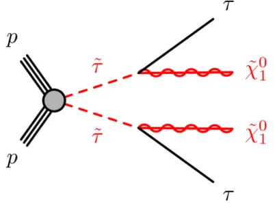
The search for directHτproduction is especially motivated by cosmological consideration [45]. Ac- cording to the co-annihilation of a relatively lightHτ(m

Hτ ≤ O(1 TeV)) observable at the LHC, with the LSP, assumed to be the Hχ⁰

1, can predict the observed DM density in the universe. To design the search strategy in terms of discriminating variables, simplified signal models are used where it is assumed that theHτis directly pair produced in thepp-collisions (see Figure 4.1). EachHτthen decays exclusively

Figure 4.1: Simplified model of direct stau pair production. Each stau decays into its SM counter partτand the lightest neutralino Hχ⁰

1[46].

into the Hχ⁰

1and aτ-lepton with a proper decay length which is much shorter than the resolution of the ATLAS vertex reconstruction. The mass eigenstates ofHτ_L andHτ_R, the left- and right-handed superpartners of theτ-lepton, are assumed to be degenerated resulting in only two paramaters of the model, namelym

Hχ⁰₁ andm

Hτ.

(34)

4 Search for Direct Stau Pair Production

Since theτ-lepton itself decays inside of the beam pipe, the search is categorized by theτ-lepton decay modes, either a hadronic and a leptonic decay, called LepHad channel, or full hadronic decays, called HadHad channel. In this thesis, only the LepHad channel was been studied. The event signature, thus, is one electron or muon with opposite charge to aτjet from a hadronically decayingτ-lepton and large missing transverse momentum.

4.1 Previous Searches

The four experiments at the Large Electron-Positron Collider (LEP), ALEPH, DELPHI, L3 and OPAL, haved searched for stau production at center-of-mass energies up to 208 GeV [47]. In ae⁺e⁻dataset at

√s =208 GeV of 585 pb⁻¹no evidence has been found for directHτproduction. The corresponding exclusion contour in them

Hτ−m

Hχ⁰

1 mass plane is shown in Figure 4.2. Hτmasses below 85 GeV are excluded for neutralino masses below 40 GeV at 95 % confidence level.

Figure 4.2: Expected and observed 95 % CL exclusion regions (hatched) in the stau-neutraline mass plane from the combined measurements of the four LEP experiments (ADLO) [48].

(35)

4.2 Object and Event Selection

Events of interest contain one electron or muon, oneτ-lepton and optionally extra jets from ISR or pile-up activity. Like in the majority of the ATLAS analyses, object are selected in three stages. In the first stage, called object-preselection, electrons, muons,τ-leptons and jets are selected within the maximum detector acceptance and minimal p_T-requirement. The application of a minimal particle identification working point (WP) to the leptons already supresses a substantial amount of the background. The same energy deposits in the detector might be considered by two different reconstruction algorithms giving rise to an ambiguity between the physics objects. This ambiguity is resolved in an iterative overlap removal procedure based on the angular separation∆R_ybetween them.

Objects surviving this second stage are called baseline objects. In the final stage selection, called signal objects selection additional criteria are applied to the baseline objects to enrich the ones from primary process.

Preselected muons are medium muons with p_T > 14 GeV and |η| < 25. Anti-k_T jets calib- rated at the electromagnetic scale must havep_T > 20 GeV. Preselectedτ-lepton candidates satisfy p_T > 20 GeV and|η| <2.47. Additionally, they must be associated with 1 or 3 charged tracks. To suppress background from quark and gluon jets a minimal cut on theτ-lepton BDT score is made, corresponding to a very looseτ-lepton ID WP.

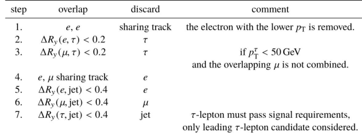
All preselected objects enter the overlap removal procedure to resolve ambiguities between the reconstruction algrorithm. In an iterative procedure objects are removed from the event if they overlap in∆Rwithin a given threshold with other physics objects optionally satifying extra properties. The full list of rules can be found in Table 4.1. All objects surviving the overlap removal are called baseline objects.

In the final selection stage, extra criteria are applied to select leptons and jets from the primary process. The longitudinal impact parameter of signal electrons to the primary vertex,|z₀·sinθ|must be less than 0.5 mm and the relative uncertainty on the transversal impact parameter measurement, d₀/σ(d₀) must be less than five. In the case of signal muons |z₀·sinθ| must be as well less than 0.5 mm and the uncertainty on the transversal impact parameter less than three. To reject leptons from hadronic activity, both electrons and muons must satisfy theFCLooseisolation criteria1. Signal jets must have∆R < 2.8. In order to reject events from secondary pile-up interactions a jet-vertexing

1Energy deposits in the ID and in the calorimeter around the letpon with a well defined cone around the lepton are summed up exluding the deposits from the lepton itself. Leptons from heavy flavour particle decays tend to have low energy deposits close-by while leptons from meson decays are usually accompanied by other hadrons resulting in large values of the isolation variables.

(36)

Table 4.1: Overlap removal requirement applied to preselected objects before the final signal selection criteria

step overlap discard comment

1. e,e sharing track the electron with the lowerp_Tis removed.

2. ∆R_y(e, τ) <0.2 τ

3. ∆R_y(µ, τ) <0.2 τ ifp^τ

T <50 GeV

and the overlappingµis not combined.

4. e, µsharing track e 5. ∆R_y(e,jet) <0.4 e 6. ∆R_y(µ,jet) <0.4 µ

7. ∆R_y(τ,jet) < 0.4 jet τ-lepton must pass signal requirements, only leadingτ-lepton candidate considered.

algorithm is applied. Signal jets must have a JVT-score larger than 0.5. Finally, baselineτ-leptons satisfying theTightidentification criteria are called signal.

Event selection

Besides the objects, events must also satisfy several quality criteria in order to be considered.

• No bad µ. The event has no baselineµwith a relative error onq/pgreater than 0.2.

• No cosmic µ: d₀> 0.2 mm andz₀ >1 mm for baselineµ.

• Bad jet: No preselected jet is mismeasured [49].

• At least one vertex with five associated tracks withp_T > 0.4 GeV.

• The event is fired by one trigger which is matched to the lepton as described in Section 4.3.

• Real data events are recorded under stable detector conditions.

4.3 Trigger strategy

Single lepton (SLT) and combined lepton-tau (TLT) triggers were used to select the events for the analysis. The LHC slowly ramped the instantaneous luminosity to 2×10⁻³⁴cm⁻¹s⁻¹by optimizing the beam parameters. To ensure that the data-recording rate maintains the same level thep_Tthresholds on the single lepton trigger hat to be increased as well. Signal leptons are requiered to be matched to the online trigger within∆R< 0.1. An additional cut on the leptonp_T, which is 1(5) GeV above the nominal treshhold for electrons (τ-leptons) and for µ5 %, to guarantee that only events where the trigger is fully efficient are selected.

(37)

4.3 Trigger strategy

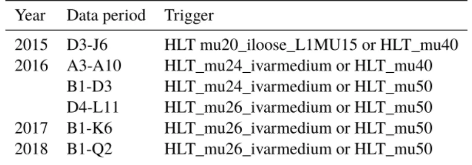
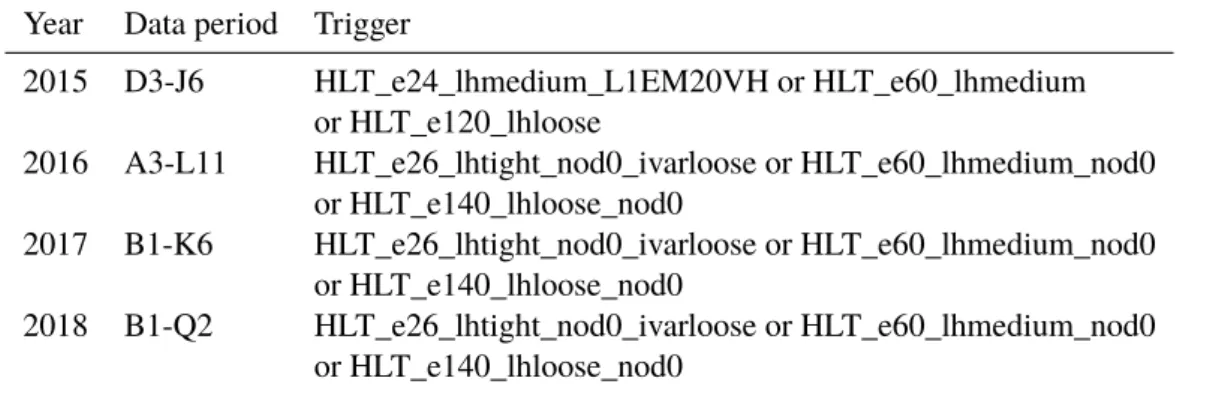
Table 4.2: Single lepton triggers requirements for muons used for different data periods

Year Data period Trigger

2015 D3-J6 HLT mu20_iloose_L1MU15 or HLT_mu40 2016 A3-A10 HLT_mu24_ivarmedium or HLT_mu40

B1-D3 HLT_mu24_ivarmedium or HLT_mu50 D4-L11 HLT_mu26_ivarmedium or HLT_mu50 2017 B1-K6 HLT_mu26_ivarmedium or HLT_mu50 2018 B1-Q2 HLT_mu26_ivarmedium or HLT_mu50

The triggers are exclusively applied to different phase-space region, defined by the transverse momentum of the lepton or/and the τ-lepton candidates. The trigger strategy of the analysis is diagrammatically depicted in Figure 4.3. The point is that single lepton triggers limit the phase space to roughly 25 GeV. The requirement of having two objects in the final state allows to have lower lepton p_T. This path is gone via the TLT.

A summary of the triggers used by each channel is reported in Tables 4.2-4.5. Any significant changes to either the detector configuration/calibration or to the trigger should usually cause the definition of a new period. For every run period at the LHC the lowest unprescaled triggers were used to be as inclusive as possible with the trigger selection. The explanation of the trigger names is explained in the following. The name starts with the specification of the trigger level, here always HLT for High Level Trigger. This is followed by the name of the selected object to which the trigger is applied: e for electron, µfor muon and tau for τ-lepton. The p_T threshold in GeV which the respective object must fulfill is then appended to the name in order for the trigger to fire. So, for example HLT_e24 is a High Level Trigger that fires if an electron with anp_T higher than 24 GeV is detected. In addition to the p_T threshold additional requirements can be imposed on an object.

The criteria ’lhloose’, ’lhmedium’ and ’lhtight’ requires that an electron passed the corresponding likelihood based selection criteria loose/medium/tight. The nod0 requirement shows that no transverse impact parameter cuts are required. The specifiers ’ivarloose’ and ’ivarmedium’ indicate a variable sized cone isolation requirement. The ’L1EM20VH’ criteria requires that an electromagnetic (EM) object has ap_Thigher than 20 GeV at L1. The ’V’ indicates a pseudorapidity dependent transverse energy threshold and the ’H’ indicates hadronic isolation[50]. The ’L1MU15’ criteria requires that a muon has a p_T higher than 15 GeV at L1. The ’iloose’ criteria indicate a loose track isolation requirement [51]. The ’tracktwo’ criterium requiresτ-lepton objects to have one or three charged tracks and ’medium1’ indicates that a BDT algorithm selected the tau according to the ’medium’ level of purity [52].

(38)

Table 4.3: Single lepton triggers requirements for electrons used for different data periods

Year Data period Trigger

2015 D3-J6 HLT_e24_lhmedium_L1EM20VH or HLT_e60_lhmedium or HLT_e120_lhloose

2016 A3-L11 HLT_e26_lhtight_nod0_ivarloose or HLT_e60_lhmedium_nod0 or HLT_e140_lhloose_nod0

2017 B1-K6 HLT_e26_lhtight_nod0_ivarloose or HLT_e60_lhmedium_nod0 or HLT_e140_lhloose_nod0

2018 B1-Q2 HLT_e26_lhtight_nod0_ivarloose or HLT_e60_lhmedium_nod0 or HLT_e140_lhloose_nod0

Table 4.4: Combined lepton-tau triggers requirements for muons and taus used for different data periods

Year Data period lepton trigger tau trigger

2015 D3-J6 HTL_mu14 HTL_tau35_medium1_tracktwo

2016 A3-A10 HLT_mu14_ivarloose HTL_tau35_medium1_tracktwo 2016 B1-D3 HLT_mu14_ivarloose HTL_tau35_medium1_tracktwo 2016 D4-L11 HLT_mu14_ivarloose HTL_tau35_medium1_tracktwo 2017 B1-K6 HLT_mu14_ivarloose HTL_tau35_medium1_tracktwo 2018 B1-H2 HLT_mu14_ivarloose HTL_tau35_medium1_tracktwoEF 2018 I1-Q2 HLT_mu14_ivarloose HTL_tau35_medium1_tracktwoEF

Table 4.5: Combined lepton-tau triggers requirements for electrons and taus used for different data periods

Year Data period lepton trigger tau trigger

2015 D3-J6 HLT_e24_lhmedium_L1EM20VH tau80_medium1_tracktwo 2016 A3-L11 HLT_e26_lhtight_nod0_ivarloose tau80_medium1_tracktwo 2017 B1-K6 HLT_e26_lhtight_nod0_ivarloose tau80_medium1_tracktwo 2018 B1-Q2 HLT_e26_lhtight_nod0_ivarloose tau80_medium1_tracktwo

(39)

4.3 Trigger strategy

Figure 4.3: Schematic of the trigger strategy used in the analysis.

(40)

(41)

CHAPTER FIVE

MONTE CARLO DATA SAMPLE

MC simulations are used in the analysis in order to model both the known SM background processes based on the SM theory and the signal samples based on the MSSM theory. The MC samples are designed to model the data conditions. This includes information about the pile-up conditions and the triggers used for the data acquisition.

Signal samples:

Within the MSSM, stau pairs can be produced directly at the LHC via pp→HτHτ. The simulation of the tree-level matrix element is done with the MadGraph program and the simulation of parton shower and hadronization is done with Pythia8. The A14 tuning series in combination with the N23LO parton density function is applied to tune the free parameters. The signal mass point grid is spanned by different stau and neutralino masses. 52 different mass points, fromm

Hτ =80 GeV up tom

Hτ = 440 GeV in 40 GeV steps andm

χH¹

0 =1 GeV up tom

χH¹

0 =200 GeV were generated. The full signal grid of simulated signal samples is shown in Figure 5.1. Each sample is divided into two different subprocesses. The first subprocess contains the production of the two stau mass eigenstatesHτ₁ assigned to the purely left-handed weak eigenstateHτ_L. The second subprocess contains the production of the two stau mass eigenstatesHτ₂assigned to the purely right-handed weak eigenstateHτ_R. The mixing of both stau mass eigenstates as well as a mass splitting between them are not taken into account.

Table A1 and Table A2 summarize the different mass points and Figure 5.1 shows the graphical arrangement of the mass points depending on the stau and LSP mass.

(42)

5 Monte Carlo Data Sample

Figure 5.1: Signal mass points available in this analysis.

. Background samples:

SM processes which have either the same (irreducible) or similar (reducible) signature in the detector and therefore mimic the signal detector signature is referred to as background. This can happen if a SM process shares the same final state particle as the signal model or by a misreconstruction which gives the same final state particle. All background processes are classified into five different categories:

W+jets,Z →``,Z →ττ, Top and Others.

W+jets:

The production of a W boson in association with "jets", initiated by quarks or gluons are referred to as W+jets. Such events have an attractive signature for many fundamental tests of the SM. The W+jets processes also provide the main background for many studies beyond the SM. When investigateing the lepton-hadron channel the W+jets is classified depending on the decay channel as reducible (W →`ν)

(43)

or irreducible (W →τν). For both cases a significant lack of energy can be generated by the escaping neutrinos. W+jets samples are simulated with Sherpa v2.2.1 and the NNPDF30NNLO PDF set. A possible process of W+jets at tree level is shown in Figure 5.2.

W⁻

g

¯ q q

¯ ν ℓ⁻

Figure 5.2: W+jets production at leading order.

. Z →ττ:

The production of a Z boson that decays into two opposite chargedτ-leptons, denoted asZ →ττ, is classified as reducible background if one of theτ-lepton can decays leptonically and the other one hadronically. This process also provides interesting searches forττfinal states. Missing energy can be generated due to the escaping neutrinos. Z →ττsamples are simulated with Sherpa v2.2.1 and the NNPDF30NNLO PDF set. Figure 5.3 shows the main Feynman diagramZ →ττprocess at tree level.

¯ q q

Z

τ⁺

τ⁻

Figure 5.3: Feynman diagram at tree level for theZproduction and decays into a pair ofτ-leptons.

. Z →``:

The production of a Z boson which decays leptonically, either in two opposite charged electrons (Z → ee) or in two opposite charged muons (Z → µµ), denoted as Z → ``, are reducible back-

(44)

5 Monte Carlo Data Sample

grounds. Z →``pass the signal preselection only if one lepton is reconstructed as a fake tau. Z →``

samples are like the previous samples simulated with Sherpa v2.2.1 and the NNPDF30NNLO PDF set.

Top:

The Top category includes all events in which single top ort¯tis produced: single top,tt¯,t Z→3`,t¯ttt¯ andt¯tV (t¯tincludes the electroweak process with boson radiation: t¯t Zandt¯tW) production. All of them are classified as reducible background processes. Top quarks decays almost every time into aW boson and abquark. Therefore, it can be heavily supressed by the requirement of zero b-jets in the event. Single top,tt¯,t Z →3`andt¯ttt¯samples are generated with Powheg and Pythia v8.2 and the ttV sample is simulated via Sherpa. Figure 5.5 shows representative Feynman diagrams at tree level for the single top and onett¯process, respectively.

g b

b

W⁻

t

g g

g

¯t

t

Figure 5.4: Feynman diagram for the single top production in theW tchannel (left) and thet¯tprocess viagg fusion (right).

Others:

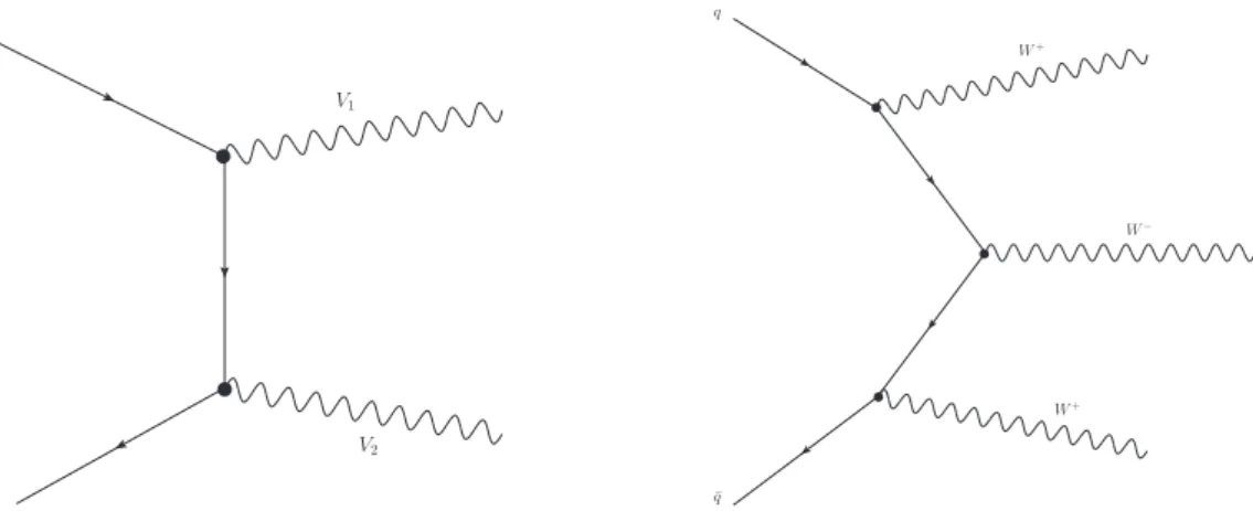
The production of two electroweak bosons, referred to as diboson, or three electroweak bosons, referred to as triboson and the Higgs production are captured in the "Others" category. Diboson decay modes:

Z Z →ττνν,W W →τντνandW W →τν`νand the trisboson decay mode: Z Z Z →ττννννhave the same final state signature as the signal process and are therefore treated as irreducible backgrounds.

Diboson samples are generated with Sherpa v2.2.1 and triboson samples with Sherpa v2.2.2. The associated production of a Higgs boson and a top quark-antiquark pair (tt Hproduction) is simulated with aMC@NLO, Pythia v8.2 and EvtGen. Higgs production via vector-boson fusion (VBF) and via gluon-gluon fusion (ggH) is simulated with Powheg, Pythia v8.2 and EvtGen. Figure 5.5 shows a possible diboson and triboson process.

5.1 SM background Modelling at Preselection

The modeling of the MC generators can be initially checked at the preselection stage. The preselection possesses higher statistics compared to the control regions and is therefore more trustworthy in case of

(45)

5.1 SM background Modelling at Preselection

q

¯ q

V₁

V₂

q

¯ q

W⁺

W⁻

W⁺

Figure 5.5: Feynman diagrams at leading order for the diboson production in thet-channel (left) and the driboson process (right).

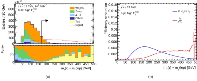
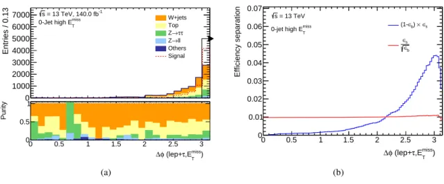
mismodelling. Figure 5.6 shows the modelling of four kinematic variables: M_T(`,E_T^miss)+M_T(τ,E_T^miss), E^miss

T ,m_effandM_T^max

2 . Figure 5.7 shows the two angular variables: ∆φ(`, τ) and∆η(`, τ). Figure 5.8 the first two unnormalized Fox-Wolfram moments and Figure 5.9 the mass of the recursive jigsawZ boson andWboson candidate. All variables, introduced in Section 6.2, shows the same behaviour.

The MC generators underestimate Data. The missing contributions from MC simulations to data can be explained by the missing QCD multijet background. This missing background is especially expected for lowE^miss

T values as shown in Figure 5.6(c). Since no QCD multijet background estimation has yet been performed, the MC simulations cannot be validated accurately.