ATLAS-CONF-2012-080 07July2012
ATLAS NOTE
ATLAS-CONF-2012-080
July 3, 2012
Improved Luminosity Determination in pp Collisions at √
s = 7 TeV using the ATLAS Detector at the LHC
The ATLAS Collaboration
Abstract
The luminosity calibration for the ATLAS detector at the LHC during ppcollisions at
√s=7 TeV in 2010 and 2011 is presented. Evaluation of the luminosity scale is performed
using several luminosity-sensitive detectors, and comparisons of the long-term stability and accuracy of this calibration applied to the ppcollisions at √
s= 7 TeV are made. A relative luminosity uncertainty ofδL/L = ±3.4% is obtained for the 48 pb−1 of data delivered to ATLAS in 2010, and a relative uncertainty ofδL/L = ±1.8% is obtained for the 5.6 fb−1 delivered in 2011.
c
Copyright 2012 CERN for the benefit of the ATLAS Collaboration.
Reproduction of this article or parts of it is allowed as specified in the CC-BY-3.0 license.
1 Introduction
An accurate measurement of the delivered luminosity is a key component of the ATLAS [1] physics program. For cross-section measurements, the uncertainty on the delivered luminosity is often one of the dominant systematic uncertainties. Searches for, and eventual discoveries of, new physical phenomena beyond the Standard Model also rely on accurate information about the delivered luminosity to evaluate background levels and determine sensitivity to the signatures of new phenomena.
This paper describes the measurement of the luminosity delivered to the ATLAS detector at the LHC in ppcollisions at a center-of-mass energy of √
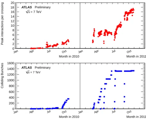
s = 7 TeV during 2010 and 2011. The analysis is an evolution of the process documented in the initial ATLAS luminosity publication [2] and includes an improved determination of the luminosity in 2010 along with a new analysis for 2011. Table 1 high- lights the operational conditions of the LHC during 2010 and 2011. The peak instantaneous luminosity delivered by the LHC at the start of a fill has increased from Lpeak = 2.0×1032cm−2s−1 in 2010 to Lpeak = 3.6×1033cm−2s−1 by the end of 2011. This increase results from both an increased instan- taneous luminosity delivered per bunch crossing as well as a significant increase in the total number of bunches colliding. Figure 1 illustrates the evolution of these two parameters as a function of time. As a result of these changes in operating conditions, the details of the luminosity measurement have evolved from 2010 to 2011, although the overall methodology remains largely the same.
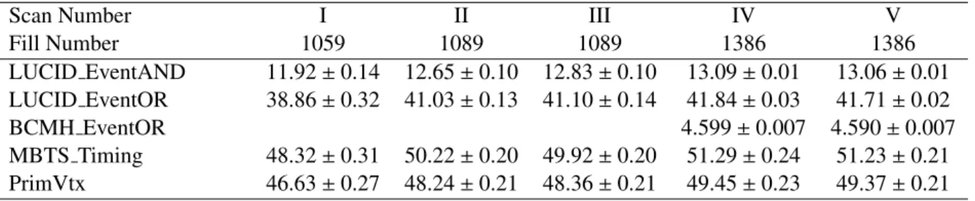
Parameter 2010 2011
Maximum number of bunch pairs colliding 348 1331
Minimum bunch spacing (ns) 150 50
Typical bunch population (1011protons) 0.9 1.2 Peak luminosity (1033cm−2s−1) 0.2 3.6 Maximum inelastic interactions per crossing ∼5 ∼20 Total integrated luminosity delivered 48 pb−1 5.6 fb−1 Table 1: Selected LHC parameters forppcollisions at √
s=7 TeV in 2010 and 2011. Parameters shown are the best achieved for that year in normal physics operations.
The ATLAS strategy for measuring and calibrating the luminosity is outlined in Section 2, followed in Section 3 by a brief description of the detectors used for luminosity determination. Each of these detectors utilizes one or more luminosity algorithms as described in Section 4. The absolute calibration of these algorithms using beam-separation scans is described in Section 5, while a summary of the systematic uncertainties on the luminosity calibration as well as the calibration results are presented in Section 6. Additional corrections which must be applied over the course of the 2011 data-taking period are described in Section 7, while additional uncertainties related to the extrapolation of the absolute luminosity calibration to the full 2010 and 2011 data samples are described in Section 8. The final results and uncertainties are summarized in Section 9.
2 Overview
The luminosity of appcollider can be expressed as L= Rinel
σinel (1)
whereRinelis the rate of inelastic collisions andσinelis theppinelastic cross-section. For a storage ring, operating at a revolution frequency fr and withnbbunch pairs colliding per revolution, this expression
Month in 2010 Month in 2011
Jan Apr Jul Oct Jan Apr Jul Oct
Peak interactions per crossing
0 2 4 6 8 10 12 14 16 18 20
= 7 TeV s
ATLAS Preliminary
Month in 2010 Month in 2011
Jan Apr Jul Oct Jan Apr Jul Oct
Colliding Bunches
0 200 400 600 800 1000 1200 1400 1600
= 7 TeV s
ATLAS Preliminary
Figure 1: Average number of inelastic ppinteractions per bunch crossing at the start of each LHC fill (above) and number of colliding bunches per LHC fill (below) are shown as a function of time in 2010 and 2011. The product of these two quantities is proportional to the peak luminosity at the start of each fill.
can be rewritten as
L= µnbfr
σinel (2)
whereµis the average number of inelastic interactions per bunch crossing (BC).
As will be discussed in Sections 3 and 4, ATLAS monitors the delivered luminosity by measuring the observed interaction rate per crossing, µvis, independently with a variety of detectors and using several different algorithms. The luminosity can then be written as
L= µvisnbfr
σvis (3)
where σvis = εσinel is the total inelastic cross-section multiplied by the efficiency ε of a particular detector and algorithm, and similarlyµvis =εµ. Sinceµvisis an experimentally observable quantity, the calibration of the luminosity scale for a particular detector and algorithm is equivalent to determining the visible cross-sectionσvis.
The majority of the algorithms used in the ATLAS luminosity determination are event counting algorithms, where each particular bunch crossing is categorized as either passing or not passing a given set of criteria designed to detect the presence of at least one inelasticppcollision. In the limitµvis 1, the average number of visible inelastic interactions per BC is given by the simple expression µvis ≈ N/NBC where N is the number of bunch crossings (or events) passing the selection criteria that are observed during a given time interval, and NBC is the total number of bunch crossings in that same interval. As µvis increases, the probability that two or more pp interactions occur in the same bunch crossing is no longer negligible (a condition referred to as “pile-up”), and µvis is no longer linearly related to the raw event count N. Insteadµvismust be calculated taking into account Poisson statistics,
and in some cases instrumental or pile-up related effects. In the limit where all bunch crossings in a given time interval contain an event, the event counting algorithm no longer provides any useful information about the interaction rate.
An alternative approach, which is linear to higher values ofµvisbut requires more effort to control systematic effects, is that ofhit countingalgorithms. Rather than just counting how many bunch crossings pass some minimum criteria for containing at least one inelastic interaction, in hit counting algorithms the number of detector readout channels with signals above some predefined threshold is counted. This provides more information per event, and also increases the µvis value at which the algorithm saturates compared to an event-counting algorithm. The extreme limit of hit counting algorithms, achievable only in detectors with very fine segmentation, are particle counting algorithms, where the number of individual particles entering a given detector is counted directly. More details on how these different algorithms are defined, as well as the procedures for converting the observed event or hit rate into the visible interaction rateµvis, are discussed in Section 4.
As described more fully in Section 5, the calibration of σvis is performed using dedicated beam separation scans, also known as van der Meer (vdM) scans, where the absolute luminosity can be inferred from direct measurements of the beam parameters [3,4]. The delivered luminosity can be written in terms of the accelerator parameters as
L= nbfrn1n2
2πΣxΣy (4)
where n1 and n2 are the bunch populations (protons per bunch) in beam 1 and beam 2 respectively (together forming the bunch population product), andΣx andΣycharacterize the horizontal and vertical convolved beam widths. In a vdMscan, the beams are separated by steps of a known distance which allows a direct measurement of Σx andΣy. Combining this scan with an external measurement of the bunch population product n1n2 provides a direct determination of the luminosity when the beams are unseparated.
A fundamental ingredient of the ATLAS strategy to assess and control the systematic uncertainties affecting the absolute luminosity determination is to compare the measurements of several luminosity detectors, most of which use more than one algorithm to assess the luminosity. These multiple detectors and algorithms are characterized by significantly different acceptance, response to pile-up, and sensitiv- ity to instrumental effects and to beam-induced backgrounds. In particular, since the calibration of the absolute luminosity scale is established in dedicatedvdM scans which are carried out relatively infre- quently (in 2011 there was only onevdMscan at √
s = 7 TeV for the entire year), this calibration must be assumed to be constant over long periods and under different machine conditions. The level of consis- tency across the various methods, over the full range of single-bunch luminosities and beam conditions, and across many months of LHC operation, provides valuable cross-checks as well as an estimate of the detector-related systematic uncertainties. A full discussion of these is presented in Sections 6 to 8.
The information needed for most physics analyses is an integrated luminosity for some well defined data sample. The basic time unit for storing luminosity information for physics use is the Luminosity Block(LB). The boundaries of each LB are defined by the ATLAS Central Trigger Processor (CTP), and in general the duration of each luminosity block is around one minute. Trigger configuration changes, such as prescale changes, can only happen at luminosity block boundaries, and data are analyzed un- der the assumption that each luminosity block contains data taken under uniform conditions, including luminosity. The average luminosity for each detector and algorithm, along with a variety of general AT- LAS data quality information, is stored in a relational database for each LB. To define a data sample for physics, quality criteria are applied to remove LBs where conditions are not acceptable, then the average luminosity in that LB is multiplied by the LB duration to provide the integrated luminosity delivered in that LB. Additional corrections can be made for trigger deadtime and trigger prescale factors, which are also recorded on a per-LB basis. Adding up the integrated luminosity delivered in a specific set of
luminosity blocks provides the integrated luminosity of the entire data sample.
3 Luminosity Detectors
This section provides a brief description of the detector subsystems used for luminosity measurements.
The ATLAS detector is discussed in detail in [1]. The first set of detectors uses either event or hit counting algorithms to measure the luminosity on a bunch-by-bunch basis. The second set infers the total luminosity (summed over all bunches) by monitoring detector currents sensitive to average particle rates over longer time scales. In each case, the detector descriptions are arranged in order of increasing magnitude of pseudorapidity.1
The Inner Detector (ID) is used to measure the momentum of charged particles over a pseudorapid- ity interval of|η| < 2.5. It consists of three subsystems: a pixel detector, a silicon strip tracker, and a transition-radiation straw-tube tracker. These detectors are located inside a solenoidal magnet that pro- vides a 2 T axial field. The tracking efficiency as a function of transverse momentum (pT), averaged over all pseudorapidity, rises from 10% at 100 MeV to around 86% for pT above a few GeV [5, 6]. The main application of the Inner Detector for luminosity measurements is to detect the primary vertices produced in inelastic ppinteractions.
For the initial LHC running period at low instantaneous luminosity (L<1033cm−2s−1), ATLAS has been equipped with segmented scintillator counters, the Minimum Bias Trigger Scintillators (MBTS), located at z = ±365 cm from the nominal interaction point (IP), and covering a rapidity range 2.09 <
|η|< 3.84. The main purpose of the MBTS is to provide a trigger on minimum collision activity during a ppbunch crossing. Light emitted by the scintillators is collected by wavelength-shifting optical fibers and guided to photomultiplier tubes. The MBTS signals, after being shaped and amplified, are fed into leading-edge discriminators and sent to the ATLAS trigger system. The MBTS is primarily used for luminosity measurements in early 2010, and is no longer used in the 2011 data.
The Beam Conditions Monitor (BCM) consists of four small diamond sensors, approximately 1 cm2 in cross-section, arranged around the beampipe in a cross pattern on each side of the IP, at a distance of z = ±184 cm . The BCM is a fast device originally designed to monitor background levels and issue beam-abort requests when beam losses start to risk damaging the Inner Detector. The fast readout of the BCM also provides a bunch-by-bunch luminosity signal at|η| = 4.2 with a time resolution of' 0.7 ns.
The horizontal and vertical pairs of BCM detectors are read out separately, leading to two luminosity measurements labelled BCMH and BCMV respectively. Because the acceptances, thresholds, and data paths may all have small differences between BCMH and BCMV, these two measurements are treated as being made by independent devices for calibration and monitoring purposes, although the overall response of the two devices is expected to be very similar. In the 2010 data, only the BCMH readout is available for luminosity measurements, while both BCMH and BCMV are available in 2011.
LUCID is a Cherenkov detector specifically designed for measuring the luminosity in ATLAS. Six- teen mechanically polished aluminum tubes filled with C4F10 gas surround the beampipe on each side of the IP at a distance of 17 m, covering the pseudorapidity range 5.6 < |η| < 6.0. The Cherenkov photons created by charged particles in the gas are reflected by the tube walls until they reach photomul- tiplier tubes (PMTs) situated at the back end of the tubes. Additional Cherenkov photons are produced in the quartz window separating the aluminum tubes from the PMTs. The Cherenkov light created in the gas typically produces 60-70 photoelectrons per incident charged particle, while the quartz window
1ATLAS uses a coordinate system where the nominal interaction point is at the center of the detector. The direction of beam 2 (counterclockwise around the LHC ring) defines thez-axis; thex-yplane is transverse to the beam. The positivex-axis is defined as pointing to the center of the ring, and the positivey-axis upwards. Side-A of the detector is on the-positivezside and side-C on the negative-zside. The azimuthal angleφis measured around the beam axis. The pseudorapidityηis defined as η=−ln(tanθ/2) whereθis the polar angle from the beam axis.
adds another 40 photoelectrons to the signal. If one of the LUCID PMTs produces a signal over a preset threshold (equivalent to'15 photoelectrons), a “hit” is recorded for that tube in that bunch crossing. The LUCID hit pattern is processed by a custom-built electronics card which contains Field Programmable Gate Arrays (FPGAs) that can be programmed with different luminosity algorithms, and provide separate luminosity measurements for each LHC bunch crossing.
Both BCM and LUCID are fast detectors with electronics capable of making statistically precise lu- minosity measurements separately for each bunch crossing within the LHC fill pattern with no deadtime.
These FPGA-based front-end electronics run autonomously from the main ATLAS data acquisition sys- tem, and in particular are not affected by any deadtime imposed by the ATLAS CTP. The ID vertex data and the MBTS data are components of the events read out through the central ATLAS trigger system, and so must be corrected for deadtime imposed by the CTP in order to measure delivered luminosity.
Normally this deadtime is below 1%, but can occasionally be larger. Since not every inelastic collision event can be read out through the ATLAS trigger system, the bunch crossings are sampled with a random or minimum bias trigger. While the triggered ATLAS events uniformly sample every bunch crossing, the trigger bandwidth devoted to random or minimum bias triggers is not large enough to measure the luminosity separately for each bunch pair in a given LHC fill pattern during normal physics operations.
For special running conditions such as the vdMscans, a custom trigger with partial event readout has been introduced in 2011 to record enough data to allow bunch-by-bunch luminosity measurements from the ATLAS ID.
In addition to the detectors listed above, further luminosity-sensitive methods have been developed which use components of the ATLAS calorimeter system. These techniques do not identify particular events, but rather measure average particle rates over longer time scales.
The Tile Calorimeter (TileCal) is the central hadronic calorimeter of ATLAS. It is a sampling calorime- ter constructed from iron plates (absorber) and plastic tile scintillators (active material) covering the pseudorapidity range|η| < 1.7. The detector consists of three cylinders, a central long barrel and two smaller extended barrels, one on each side of the long barrel. Each cylinder is divided into 64 slices in φ(modules) and segmented into three radial sampling layers. Cells are defined in each layer according to a projective geometry, and each cell is connected by optical fibers to two photomultiplier tubes. The current drawn by each PMT is monitored by an integrator system which is sensitive to currents from 0.1 nA to 1.2 mA with a time constant of 10 ms. The current drawn is proportional to the total number of particles interacting in a given TileCal cell, and provides a signal proportional to the total luminosity summed over all the colliding bunches present at a given time.
The Forward Calorimeter (FCal) is a sampling calorimeter that covers the pseudorapidity range 3.2<
|η| < 4.9 and is housed in the two end-cap cryostats along with the electromagnetic end-cap and the hadronic end-cap calorimeters. Each of the two FCal modules is divided into three longitudinal absorber matrices, one made of copper (FCal-1) and the other two of tungsten (FCal-2/3). Each matrix contains tubes arranged parallel to the beam axis filled with liquid argon as the active medium. Each FCal-1 matrix is divided into 16φ-sectors, each of them fed by four independent high-voltage lines. The high voltage on each sector is regulated to provide a stable electric field across the liquid argon gaps and, similar to the TileCal PMT currents, the currents provided by the FCal-1 high-voltage system are directly proportional to the average rate of particles interacting in a given FCal sector.
4 Luminosity Algorithms
This section describes the algorithms used by the luminosity-sensitive detectors described in Section 3 to measure the visible interaction rate per bunch crossing,µvis. Most of the algorithms used do not measure µvisdirectly, but rather measure some other rate which can be used to determineµvis.
ATLAS primarily uses event counting algorithms to measure luminosity, where a bunch crossing is
said to contain an “event” if the criteria for a given algorithm to observe one or more interactions are satisfied. The two main algorithm types being used are EventOR (inclusive counting) and EventAND (coincidence counting). Since in general there can be more than one ppinelastic collision per bunch crossing, the visible interaction rateµvis is a linear function of the event rate only whenµvis 1, and in general µvis must be determined from the observed event rates using the formulae described below.
Additional algorithms have been developed using hit counting and average particle rate counting which provide a cross-check of the linearity of the event counting techniques.
4.1 Interaction Rate Determination
Most of the primary luminosity detectors in ATLAS consist of two symmetric detector elements placed in the forward (“A”) and backward (“C”) direction from the interaction point. For the LUCID, BCM, and MBTS detectors, each side is further segmented into a discrete number of readout segments, typically arranged azimuthally around the beampipe, each with a separate readout channel. For event counting algorithms, a threshold is applied to the analog signal output from each readout channel, and every channel with a response above this threshold is counted as containing a “hit”.
In an EventOR algorithm, a bunch crossing will be counted if there is at least one hit on either the A side or the C side. Assuming that the number of interactions in a bunch crossing can be described by a Poisson distribution, the probability of observing an OR event can be computed as
PEvent OR(µORvis) = NNORBC
= 1−e−µORvis. (5)
Here the raw event countNORis the number of bunch crossings, during a given time interval, in which at least one ppinteraction satisfies the event-selection criteria of the OR algorithm under consideration, andNBCis the total number of bunch crossings during the same interval. Solving forµvisin terms of the event-counting rate yields:
µORvis =−ln 1− NNOR
BC
. (6)
In the case of an EventAND algorithm, a bunch crossing will be counted if there is at least one hit on both sides of the detector. This coincidence condition can be satisfied either from a singleppinteraction or from individual hits on either side of the detector from different ppinteractions in the same bunch crossing. Assuming equal acceptance for sides A and C, the probability of recording an AND event can be expressed as
PEvent AND(µANDvis ) = NNANDBC
= 1−2e−(1+σORvis/σANDvis )µANDvis /2+e−(σORvis/σANDvis )µANDvis . (7) This relationship cannot be inverted analytically to determine µANDvis as a function of NAND/NBC so a numerical inversion is performed instead.
When µvis 1, event counting algorithms lose sensitivity as fewer and fewer events in a given time interval have bunch crossings with zero observed interactions. In the limit whereN/NBC = 1, it is no longer possible to use event counting to determine the interaction rateµvis, and more sophisticated techniques must be used. One example is ahit countingalgorithm, where the number of hits in a given detector is counted rather than just the total number of events. This provides more information about the interaction rate per event, and increases the luminosity at which the algorithm will saturate.
Under the assumption that the number of hits in one ppinteraction follows a Binomial distribution and that the number of interactions per bunch crossing follows a Poisson distribution one can calculate the average probability to have a hit in one of the detector channels per bunch crossing as
PHIT(µHITvis ) = NBCNHITNCH
= 1−e−µHITvis , (8)
whereNHITandNBCare the total numbers of hits and bunch crossings during a time interval, andNCHis the number of detector channels. The expression above makes it easy to calculateµHITvis from the number of hits as
µHITvis =−ln(1− NNHIT
BCNCH). (9)
Hit counting is used to analyze the LUCID response (NCH = 30) only in the high luminosity data taken in 2011. The lower acceptance of the BCM detector allows event counting to remain viable for all of 2011. The binomial assumption used to derive Equation 9 is only true if the probability to observe a hit in a single channel is independent of the number of hits observed in the other channels. A study of the LUCID hit distributions shows that this is not a correct assumption, although the data also show that Equation 9 provides a very good description of howµHITvis depends on the average number of hits.
An additional type of algorithm that can be used is aparticle countingalgorithm, where some ob- servable is directly proportional to the number of particles interacting in the detector. These should be the most linear of all of the algorithm types, and in principle the interaction rate is directly proportional to the particle rate. As discussed below, the TileCal and FCal current measurements are not exactly particle counting algorithms, as individual particles are not counted, but the measured currents should be directly proportional to luminosity. Similarly, the number of primary vertices is directly proportional to the lu- minosity, although the vertex reconstruction efficiency is significantly affected by pile-up as discussed below.
4.2 Online Algorithms
The two main luminosity detectors used in ATLAS are LUCID and BCM. Each of these is equipped with customized FPGA-based readout electronics which allow the luminosity algorithms to be applied
“online” in real time. These electronics provide fast diagnostic signals to the LHC (within a few seconds), in addition to providing luminosity measurements for physics use. Each colliding bunch pair can be identified numerically by a Bunch-Crossing Identifier (BCID) which labels each of the 3564 possible 25 ns slots in one full revolution of the nominal LHC fill pattern. The online algorithms measure the delivered luminosity independently in each BCID.
For the LUCID detector, the two main algorithms are the inclusive LUCID EventOR and the coin- cidence LUCID EventAND. In each case, a hit is defined as a PMT signal above a predefined threshold which is set lower than the average single particle response. There are two additional algorithms defined, LUCID EventA and LUCID EventC, which require at least one hit on either the A or C side respec- tively. Events passing these LUCID EventA and LUCID EventC algorithms are subsets of the events passing the LUCID EventOR algorithm, and these single-sided algorithms are used primarily to moni- tor the stability of the LUCID detector and measure certain beam-related backgrounds. There is also a LUCID HitOR hit counting algorithm which has been employed in the 2011 running to cross-check the linearity of the event counting algorithms at high values ofµvis.
For the BCM detector, there are two independent readout systems (BCMH and BCMV). A hit is defined as a single sensor with a response above the noise threshold. Inclusive OR and coincidence AND algorithms are defined for each of these independent readout systems, for a total of four BCM algorithms.
4.3 Offline Algorithms
Additional offline analyses have been performed which rely on the MBTS and the vertexing capabilities of the Inner Detector. These offline algorithms use data triggered and read out through the standard ATLAS data acquisition system, and do not have the necessary rate capability to measure luminosity independently for each BCID under normal physics conditions. Instead, these algorithms are typically used as cross checks of the primary online algorithms under special running conditions, where the trigger rates for these algorithms can be increased.
The MBTS system is used for luminosity measurements only for the data collected in the 2010 run be- fore 150 ns bunch train operation began. Events are triggered by the L1 MBTS 1 trigger which requires at least one hit in any of the 32 MBTS counters (which is equivalent to an inclusive MBTS EventOR requirement). In addition to the trigger requirement, the MBTS Timing analysis makes use of the time measurement of the MBTS detectors to select events where the time difference between the average hit times on the two sides of the MBTS satisfies|∆t|< 10 ns. This requirement is very effective at rejecting beam-induced background events, as the particles produced in these events tend to traverse the detector longitudinally resulting in large values of |∆t|, while particles coming from the interaction point will produce values of|∆t|=0. To form a∆tvalue requires at least one hit on both sides of the IP, and so in the end the MBTS Timing algorithm is in fact a coincidence algorithm.
Additional algorithms have been developed which are based on reconstructing interaction vertices formed by tracks measured in the Inner Detector. In 2010, the events were triggered by the L1 MBTS 1 trigger. The 2010 algorithm counts events with at least one reconstructed vertex, with at least two tracks with pT >100 MeV. This “primary vertex event counting” (PrimVtx) algorithm is fundamentally an in- clusive event-counting algorithm, and the conversion from the observed event rate toµvis follows Equa- tion 5.
The 2011 vertexing algorithm uses events from a trigger which randomly selects crossings from filled bunch pairs where collisions are possible. The average number of visible interactions per bunch crossing is determined by counting the number of reconstructed vertices found in each bunch crossing (Vertex).
The vertex selection criteria in 2011 were changed to require 5, 7, or 10 tracks withpT >400 MeV while also requiring tracks to have a hit in any active pixel detector module along their path.
Vertex counting suffers from nonlinear behavior with increasing interaction rates per bunch crossing, primarily due to two effects: vertex masking and fake vertices. Vertex masking occurs when the vertex reconstruction algorithm fails to resolve nearby vertices from separate interactions, decreasing the vertex reconstruction efficiency as the interaction rate increases. A data-driven correction is derived from the distribution of distances in the longitudinal direction (∆z) between pairs of reconstructed vertices. The measured distribution of longitudinal positions (z) is used to predict the expected∆zdistribution of pairs of vertices if no masking effect was present. Then, the difference between the expected and observed
∆zdistributions is related to the number of vertices lost due to masking. The procedure is checked with simulation for self-consistency at the sub-percent level, and the magnitude of the correction reaches up to+50% over the range of pile-up values in 2011 physics data. Fake vertices result from a vertex that would normally fail the requirement on the minimum number of tracks, but additional tracks from a second nearby interaction are erroneously assigned so that the resulting reconstructed vertex satisfies the selection criteria. A correction is derived from simulation and reaches -10% in 2011. Since the 2010 PrimVtx algorithm requirements are already satisfied with one reconstructed vertex, vertex masking has no effect, although fake vertices must still be corrected for.
4.4 Calorimeter-based Algorithms
The TileCal and FCal luminosity determinations do not depend upon event counting, but rather upon measuring detector currents that are proportional to the total particle flux in specific regions of the calorimeters. These particle counting algorithms are expected to be free from pile-up effects up to the highest interaction rates observed in late 2011 (µ'20).
The Tile luminosity algorithm measures PMT currents for selected cells in a region near|η| ≈ 1.25 where the largest variations in current as a function of the luminosity are observed. In 2010, the response of a common set of cells was calibrated with respect to the luminosity measured by the LUCID EventOR algorithm in a single ATLAS run. At the higher luminosities encountered in 2011, TileCal started to suffer from frequent trips of the low voltage power supplies, causing the intermittent loss of current measurements from several modules. For these data, a second method is applied, based on the calibration
of individual cells, which has the advantage of allowing different sets of cells to be used depending on their availability at a given time. The calibration is performed by comparing the luminosity measured by the LUCID EventOR algorithm to the individual cell currents at the peaks of the 2011vdMscan, as more fully described in Section 7.5. While TileCal does not provide an independent absolute luminosity measurement, it is useful for evaluating systematic uncertainties associated with both long-term stability andµ-dependence.
Similarly, the FCal high-voltage currents cannot be directly calibrated during avdMscan because the total luminosity delivered in these scans remains below the sensitivity of the current-measurement technique. Instead, calibrations were evaluated for each usable HV line independently by comparing to the LUCID EventOR luminosity for a single ATLAS run in each of 2010 and 2011. As a result, the FCal also does not provide an independently calibrated luminosity measurement, but it can be used as a systematic check of the stability and linearity of other algorithms. For both the TileCal and FCal analyses, the luminosity is assumed to be linearly proportional to the observed currents after correcting for pedestals and non-collision backgrounds.
5 Luminosity Calibration
In order to use the measured interaction rate µvis as a luminosity monitor, each detector and algorithm must be calibrated by determining its visible cross-section σvis. The primary calibration technique to determine the absolute luminosity scale of each luminosity detector and algorithm employs dedicated vdM scans to infer the delivered luminosity at one point in time from the measurable parameters of the colliding bunches. By comparing the known luminosity delivered in the vdM scan to the visible interaction rateµvis, the visible cross-section can be determined from Equation 3.
To achieve the desired accuracy on the absolute luminosity, these scans are not performed during normal physics operations, but rather under carefully controlled conditions with a limited number of colliding bunches and a modest peak interaction rate (µ . 2). At √
s = 7 TeV three sets of such scans were performed in 2010 and one set in 2011. This section describes the vdM scan procedure, while Section 6 will discuss the systematic uncertainties on this procedure and summarize the calibration results.
5.1 Absolute Luminosity from Beam Parameters
In terms of colliding-beam parameters, the luminosityLis defined (for beams colliding with zero cross- ing angle) as
L=nbfrn1n2 Z
ρˆ1(x, y) ˆρ2(x, y)dxdy (10) wherenbis the number of colliding bunch pairs, fris the machine revolution frequency (11245.5 Hz for the LHC),n1n2is the bunch population product, and ˆρ1(2)(x, y) is the normalized particle density in the transverse (x-y) plane of beam 1 (2) at the IP. Under the general assumption that the particle densities can be factorized into independent horizontal and vertical components, ( ˆρ(x, y) = ρx(x)ρy(y)), Equation 10 can be rewritten as
L=nbfrn1n2Ωx(ρx1, ρx2)Ωy(ρy1, ρy2) (11) where
Ωx(ρx1, ρx2)= Z
ρx1(x)ρx2(x)dx
is the beam overlap integral in the x direction (with an analogous definition in the y direction). In the method proposed by van der Meer [3] the overlap integral (for example in the x direction) can be
calculated as
Ωx(ρx1, ρx2)= Rx(0)
R Rx(δ)dδ, (12)
whereRx(δ) is the luminosity (or equivalentlyµvis) – at this stage in arbitrary units – measured during a horizontal scan at the time the two beams are separated by the distanceδandδ= 0 represents the case of zero beam separation.
Defining the parameterΣxas
Σx = 1
√2π
R Rx(δ)dδ,
Rx(0) . (13)
and similarly forΣy, the luminosity in Equation 11 can be rewritten as L= nbfrn1n2
2πΣxΣy (14)
which shows directly how to extract luminosity from machine parameters by performing a beam sepa- ration scan. In the case where the luminosity curve Rx(δ) is Gaussian, Σx coincides with the standard deviation of that distribution. Equation 14 is quite general;ΣxandΣy, as defined in Equation 13, depend only upon the area under the luminosity curve, and make no assumption as to the shape of that curve.
5.2 vdMScan Calibration
To calibrate a given luminosity algorithm, one can equate the absolute luminosity computed using Equa- tion 14 to the luminosity measured by a particular algorithm at the peak of the scan curve using Equa- tion 3 to get
σvis=µMAXvis 2πΣxΣy
n1n2 , (15)
whereµMAXvis is the visible interaction rate per bunch crossing observed at the peak of the scan curve as measured by that particular algorithm. Equation 15 provides a direct calibration of the visible cross- section σvis for each algorithm in terms of the peak visible interaction rateµMAXvis , the product of the convolved beam widthsΣxΣy, and the bunch population product n1n2. As discussed below, the bunch population product must be determined from an external analysis of the LHC beam currents, but the remaining parameters are extracted directly from the analysis of thevdMscan data.
For the more general case of a non-zero crossing angle, the formalism becomes considerably more involved [7], but the conclusions remain unaltered, and Equations 13 – 15 remain valid. The non-zero vertical crossing angle widens the luminosity curve by a factor that depends on the bunch length, the transverse beam size and the crossing angle, but reduces the peak luminosity by the same factor. The corresponding increase in the measured value ofΣyis exactly cancelled by the decrease inµMAXvis , so that no correction for the crossing angle is needed in the determination ofσvis.
One useful quantity that can be extracted from thevdM scan data for each luminosity method and that depends only on the transverse beam sizes, is the specific luminosityLspec:
Lspec =L/(nbn1n2)= fr
2πΣxΣy. (16)
Comparing the specific luminosity values (i.e.the inverse product of the convolved beam sizes) measured in the same scan by different detectors and algorithms provides a direct check on the mutual consistency of the absolute luminosity scale provided by these methods.
5.3 vdMScan Data Sets
The beam conditions during the dedicatedvdMscans are different from the conditions in normal physics fills, with fewer bunches colliding, no bunch trains, and lower bunch intensities. These conditions are chosen to reduce various systematic uncertainties in the scan procedure.
A total of fivevdMscans were performed in 2010, on three different dates separated by weeks or months, and an additional twovdMscans at √
s = 7 TeV were performed in 2011 on the same day to calibrate the absolute luminosity scale for ATLAS. As shown in Table 2, the scan parameters evolved from the early 2010 scans where single bunches and very low bunch charges were used. The final set of scans in 2010 and the scans in 2011 were more similar, as both used close to nominal bunch charges, more than one bunch colliding, and typical peakµvalues in the range 1.3–2.3.
Generally, eachvdMscan consists of two separate beam scans, one where the beams are separated by±6σbin thexdirection keeping the beams centered iny, and a second where the beams are separated in theydirection with the beams centered in x, where σbis the transverse size of a single beam. The beams are moved in a certain number of scan steps, then data are recorded for 20−30 seconds at each step to collect a statistically significant measurement in each luminosity detector under calibration. To help assess experimental systematic uncertainties in the calibration procedure, two sets ofvdMscans are usually taken in short succession to provide two independent calibrations under similar beam conditions.
Since the luminosity can be different for each colliding bunch pair, both because the beam sizes can vary bunch-to-bunch but also because the bunch population productn1n2can vary at the level of 10-20%, the determination ofΣx/y and the measurement ofµMAXvis at the scan peak must be performed indepen- dently for each colliding BCID. As a result, the May 2011 scan provides 14 independent measurements of σvis within the same scan, and the October 2010 scan provides 6. The agreement among the σvis values extracted from these different BCIDs provides an additional consistency check for the calibration procedure.
5.4 vdMScan Analysis
For each algorithm being calibrated, thevdMscan data are analyzed in a very similar manner. For each BCID, the specific visible interaction rateµvis/(n1n2) is plottedvs. the “nominal” beam separation,i.e.
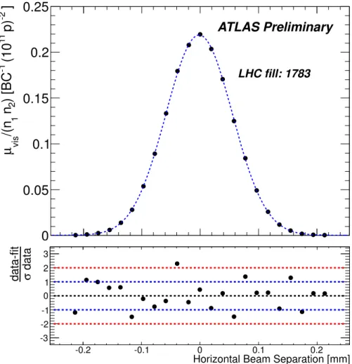
the separation specified by the LHC control system for each scan step. The specific interaction rate is used so that the result is not affected by the change in beam currents over the duration of the scan. An example of thevdMscan data for a single BCID from scan VII in thexplane is shown in Figure 2.
The value of µvis is determined from the raw event rate using the analytic function described in Section 4.1 for the inclusive EventOR algorithms. The coincidence EventAND algorithms are more in- volved, and a numerical inversion is performed to determineµvisfrom the raw EventAND rate. Since the EventANDµdetermination depends onσANDvis as well asσORvis, an iterative procedure must be employed.
This procedure is found to converge after a few steps.
Each scan for each BCID is fit independently to a characteristic function to provide a measurement ofµMAXvis from the peak of the fitted function andΣfrom the integral following Equation 13. Depending upon the beam conditions, this function can be a double Gaussian plus a constant term, a single Gaussian plus a constant term, a spline function, or other variations. As described in Section 6, the differences between the different treatments are taken into account as a systematic uncertainty in the calibration result.
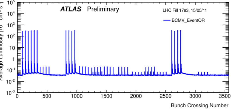
One important difference in thevdM scan analysis between 2010 and 2011 is the treatment of the backgrounds in the luminosity signals. Figure 3 shows the average BCMV EventOR luminosity as a function of BCID during the May 2011 vdMscan. The 14 large spikes around L ' 3×1029cm−2s−1 are the BCIDs containing colliding bunches. Both the LUCID and BCM detectors observe some small activity in the BCIDs immediately following a collision which tends to die away to some baseline value
vdMScanIvdMScanII–IIIvdMScanIV–VvdMScanVII–VIII (April26,2010)(May9,2010)(1October,2010)(15May,2011) LHCFillNumber1059108913861783 ScanDirections1horizontalscan2horizontalscans2setsofhorizontalplusverticalscans followedby1verticalscanfollowedby2verticalscans TotalScanStepsperPlane27272525 (±6σb)(±6σb)(±6σb)(±6σb) ScanDurationperStep30s30s20s20s BunchescollidinginATLAS&CMS11614 Totalnumberofbunchesperbeam221938 Typicalnumberofprotonsperbunch0.1·1011 0.2·1011 0.9·1011 0.8·1011 Nominalβ-functionatIP[β? ](m)223.51.5 Approx.transversesinglebeamsizeσb(µm)45456040 Nominalhalfcrossingangle(µrad)00±100±120 Typicalluminosity/bunch(µb−1 /s)4.5·10−3 1.8·10−2 0.220.38 µ(interactions/crossing)0.030.111.32.3 Table2:Summaryofthemaincharacteristicsofthe2010and2011vdMscansperformedattheATLASinteractionpoint.Thevaluesofluminos- ity/bunchandµaregivenforzerobeamseparation.
Horizontal Beam Separation [mm]
]
-2p)
11(10
-1) [BC
2n
1/(n
visµ
0 0.05 0.1 0.15
0.2 0.25
ATLAS Preliminary
LHC fill: 1783
Horizontal Beam Separation [mm]
-0.2 -0.1 0 0.1 0.2
dataσdata-fit
-3 -2 -1 0 1 2 3
Figure 2: Specific interaction rate versus nominal beam separation for the BCMH EventOR algorithm during scan VII in thexplane for BCID 817. The residual deviation of the data from the Gaussian plus constant term fit, assuming statistical errors only, is shown in the bottom panel.
with several different time constants. This “afterglow” is most likely caused by photons from nuclear de-excitation, which in turn is induced by the hadronic cascades initiated by ppcollision products. The level of the afterglow background is observed to be proportional to the luminosity in the colliding BCIDs, and in thevdMscans this background can be estimated by looking at the luminosity signal in the BCID immediately preceding a colliding bunch pair. A second background contribution comes from activity correlated with the passage of a single beam through the detector. This “single-beam” background, seen in Figure 3 as the numerous small spikes at the 1026cm−2s−1level, is likely a combination of beam-gas interactions and halo particles which intercept the luminosity detectors in time with the main beam. It is observed that this single-beam background is proportional to the bunch charge present in each bunch, and can be considerably different between beams 1 and 2, but is otherwise uniform for all bunches in a given beam. The single-beam background underlying a collision BCID can be estimated by measuring the single-beam backgrounds in unpaired bunches and correcting for the difference in bunch charge between the unpaired and colliding bunches. Adding the single-beam backgrounds measured for beams 1 and 2 then gives an estimate for the single-beam background present in a colliding BCID. Because the single-beam background does not depend on the luminosity, this background can dominate the observed luminosity response when the beams are separated.
In 2010, these background sources were accounted for by assuming that any constant term fit to the observed scan curve is the result of luminosity-independent background sources, and has not been included as part of the luminosity integrated to extractΣx orΣy. In 2011, a more detailed background subtraction is first performed to correct each BCID for afterglow and single-beam backgrounds, then any remaining constant term observed in the scan curve has been treated as a broad luminosity signal which contributes to the determination ofΣ.
Bunch Crossing Number
0 500 1000 1500 2000 2500 3000 3500
]-1 s-2 cm27Average Luminosity [10
10-3
10-2
10-1
1 10 102
103
104
105
LHC Fill 1783, 15/05/11 BCMV_EventOR
ATLAS Preliminary
Figure 3: Average observed luminosity per BCID from BCMV EventOR in the May 2011 vdMscan.
In addition to the 14 large spikes in the BCIDs where two bunches are colliding, induced “afterglow”
activity can also be seen in the following BCIDs. Backgrounds are also observed in BCIDs with unpaired bunches due to activity related to the passage of single-beams.
The combination of one xscan and oneyscan is the minimum needed to perform a measurement ofσvis. The average value ofµMAXvis between the two scan planes is used in the determination of σvis, and the correlation matrix from each fit betweenµMAXvis andΣis taken into account when evaluating the statistical uncertainty.
Each BCID should measure the sameσvisvalue, and the average over all BCIDs is taken as theσvis measurement for that scan. Any variation inσvisbetween BCIDs, as well as between scans, reflects the reproducibility and stability of the calibration procedure during a single fill.
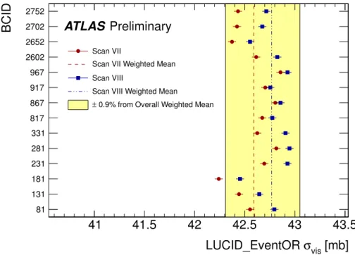
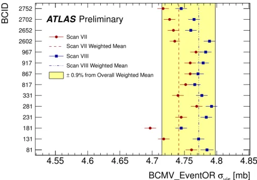
Figure 4 shows theσvisvalues determined for LUCID EventOR separately by BCID and by scan in
the May 2011 scans. The RMS variation seen between theσvis results measured for different BCIDs is 0.4% for scan VII and 0.3% for scan VIII. The BCID-averagedσvisvalues found in scans VII and VIII agree to 0.5% (or better) for all four LUCID algorithms. Similar data for the BCMV EventOR algorithm are shown in Figure 5. Again an RMS variation between BCIDs of up to 0.55% is seen, and a difference between the two scans of up to 0.67% is observed for the BCM EventOR algorithms. The agreement in the BCM EventAND algorithms is worse, with an RMS around 1%, although these measurements also have significantly larger statistical errors.
Similar features are observed in the October 2010 scan, where theσvisresults measured for different BCIDs, and the BCID-averagedσvisvalue found in scans IV and V agree to 0.3% for LUCID EventOR and 0.2% for LUCID EventAND. The BCMH EventOR results agree between BCIDs and between the two scans at the 0.4% level, while the BCMH EventAND calibration results are consistent within the larger statistical errors present in this measurement.
[mb]
σvis
LUCID_EventOR
41 41.5 42 42.5 43 43.5
BCID
81 131 181 231 281 331 817 867 917 967 2602 2652 2702 2752
Scan VII
Scan VII Weighted Mean Scan VIII
Scan VIII Weighted Mean
0.9% from Overall Weighted Mean
±
ATLAS Preliminary
Figure 4: Measured σvis values for LUCID EventOR by BCID for scans VII and VIII. The error bars represent statistical errors only. The vertical lines indicate the weighted average over BCIDs for scans VII and VIII separately. The yellow band indicates a ±0.9% variation from the average, which is the systematic uncertainty evaluated from the per-BCID and per-scanσvisconsistency.
5.5 Internal Scan Consistency
The variation between the measuredσvisvalues by BCID and between scans quantifies the stability and reproducibility of the calibration technique. Comparing Figures 4 and 5 for the May 2011 scans, it is clear that some of the variation seen inσvisis not statistical in nature, but rather is correlated by BCID.
As discussed in Section 6, the RMS variation ofσvis between BCIDs within a given scan is taken as a systematic uncertainty in the calibration technique, as is the reproducibility ofσvisbetween scans. The yellow band in these figures, which represents a range of±0.9%, shows the quadrature sum of these two systematic uncertainties. Similar results are found in the final scans taken in 2010, although with only 6 colliding bunch pairs there are fewer independent measurements to compare.
[mb]
σvis
BCMV_EventOR
4.55 4.6 4.65 4.7 4.75 4.8 4.85
BCID
81 131 181 231 281 331 817 867 917 967 2602 2652 2702 2752
Scan VII
Scan VII Weighted Mean Scan VIII
Scan VIII Weighted Mean
0.9% from Overall Weighted Mean
±
ATLAS Preliminary
Figure 5: Measuredσvis values for BCMV EventOR by BCID for scans VII and VIII. The error bars represent statistical errors only. The vertical lines indicate the weighted average over BCIDs for Scans VII and VIII separately. The yellow band indicates a ±0.9% variation from the average, which is the systematic uncertainty evaluated from the per-BCID and per-scanσvisconsistency.
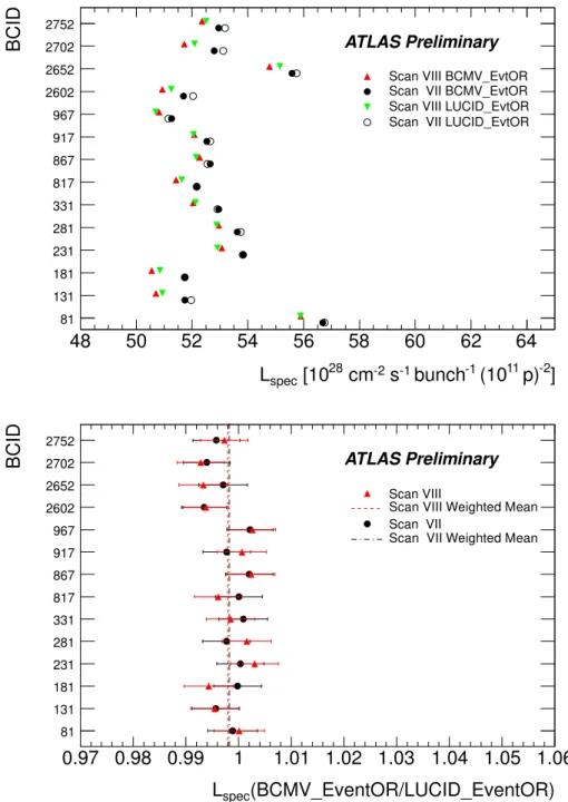
Further checks can be made by considering the distribution ofLspec defined in Equation 16 for a given BCID as measured by different algorithms. Since this quantity depends only on the convolved beam sizes, consistent results should be measured by all methods for a given scan. Figure 6 shows the measuredLspecvalues by BCID and scan for LUCID and BCMV algorithms, as well as the ratio of these values in the May 2011 scans. Bunch-to-bunch variations of the specific luminosity are typically 5–10%, reflecting bunch-to-bunch differences in transverse emittance also seen during normal physics fills. For each BCID, however, all algorithms are statistically consistent. A small systematic reduction inLspec can be observed between scans VII and VIII, which is due to emittance growth in the colliding beams.
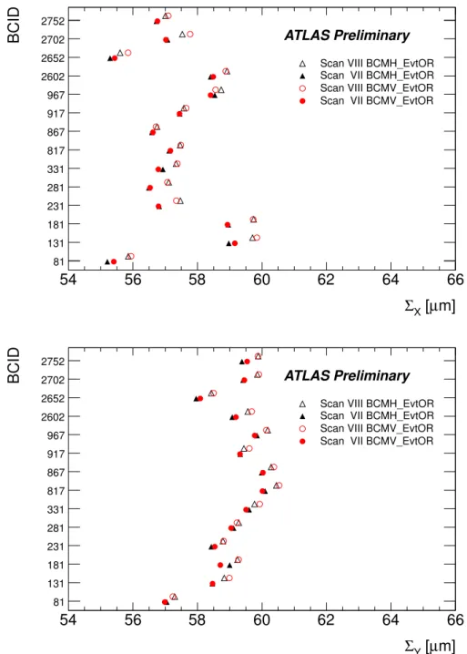
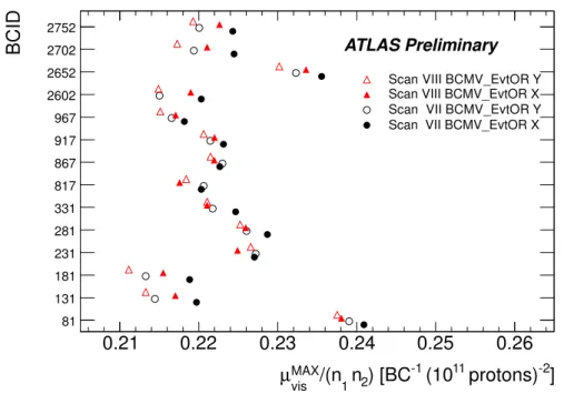
Figure 7 shows theΣx andΣyvalues determined by the BCM algorithms during scans VII and VIII, and for each BCID a clear increase can be seen with time. This emittance growth can also be seen clearly as a reduction in the peak specific interaction rateµMAXvis /(n1n2) shown in Figure 8 for BCMV EventOR.
Here the peak rate is shown for each of the four individual horizontal and vertical scans, and a monotonic decrease in rate is generally observed as each individual scan curve is recorded. The fact that the σvis values are consistent between scan VII and scan VIII demonstrates that to first order the emittance growth factors out of the measured luminosity calibration factors. The residual uncertainty associated with emittance growth is discussed in Section 6.
5.6 Bunch Population Determination
The dominant systematic uncertainty on the 2010 luminosity calibration, described in [2, 8], is associ- ated with the determination of the bunch population product (n1n2) for each colliding BCID. Since the luminosity is calibrated on a bunch-by-bunch basis for the reasons described in Section 5.3, the bunch population per BCID is necessary to perform this calibration. Measuring the bunch population prod-
-2]
11 p)
-1 (10 bunch s-1
cm-2
[1028
Lspec
48 50 52 54 56 58 60 62 64
BCID
81 131 181 231 281 331 817 867 917 967 2602 2652 2702 2752
Scan VIII BCMV_EvtOR Scan VII BCMV_EvtOR Scan VIII LUCID_EvtOR Scan VII LUCID_EvtOR
ATLAS Preliminary
(BCMV_EventOR/LUCID_EventOR) Lspec
0.97 0.98 0.99 1 1.01 1.02 1.03 1.04 1.05 1.06
BCID
81 131 181 231 281 331 817 867 917 967 2602 2652 2702 2752
Scan VIII
Scan VIII Weighted Mean Scan VII
Scan VII Weighted Mean
ATLAS Preliminary
Figure 6: Specific luminosity determined by BCMV and LUCID per BCID for scans VII and VIII.
The figure on the top shows the specific luminosity values determined by BCMV EventOR and LU- CID EventOR, while the figure on the bottom shows the ratios of these values. The vertical lines indicate the weighted average over BCIDs for scans VII and VIII separately. The error bars represent statistical uncertainties only.
m]
[µ ΣX
54 56 58 60 62 64 66
BCID
81 131 181 231 281 331 817 867 917 967 2602 2652 2702 2752
ATLAS Preliminary
Scan VIII BCMH_EvtOR Scan VII BCMH_EvtOR Scan VIII BCMV_EvtOR Scan VII BCMV_EvtOR
m]
[µ ΣY
54 56 58 60 62 64 66
BCID
81 131 181 231 281 331 817 867 917 967 2602 2652 2702 2752
Scan VIII BCMH_EvtOR Scan VII BCMH_EvtOR Scan VIII BCMV_EvtOR Scan VII BCMV_EvtOR
ATLAS Preliminary
Figure 7: Σx (top) andΣy (bottom) determined by BCM EventOR algorithms per BCID for scans VII and VIII. The statistical uncertainty on each measurement is approximately the size of the marker.
-2] protons) (1011
) [BC-1
n2
/(n1 MAX
µvis
0.21 0.22 0.23 0.24 0.25 0.26
BCID
81 131 181 231 281 331 817 867 917 967 2602 2652 2702 2752
Scan VIII BCMV_EvtOR Y Scan VIII BCMV_EvtOR X Scan VII BCMV_EvtOR Y Scan VII BCMV_EvtOR X
ATLAS Preliminary
Figure 8: Peak specific interaction rateµMAXvis /(n1n2) determined by BCMV EventOR per BCID for scans VII and VIII. The statistical uncertainty on each measurement is approximately the size of the marker.
uct separately for each BCID is also unavoidable as only a subset of the circulating bunches collide in ATLAS (14 out of 38 during the 2011 scan).
The bunch population measurement is performed by the LHC Bunch Current Normalization Working Group (BCNWG) and has been described in detail in [9, 10] for 2010 and [11–13] for 2011. A brief summary of the analysis is presented here, along with the uncertainties on the bunch population product.
The relative uncertainty on the bunch population product (n1n2) is shown in Table 3 for thevdM scan fills in 2010 and 2011.
Scan Number I II–III IV–V VII–VIII
LHC Fill Number 1059 1089 1386 1783
DCCT baseline offset 3.9% 1.9% 0.1% 0.10%
DCCT scale variation 2.7% 2.7% 2.7% 0.21%
Bunch-to-bunch fraction 2.9% 2.9% 1.6% 0.20%
Ghost charge and satellite bunches - - - 0.44%
Total 5.6% 4.4% 3.1% 0.54%
Table 3: Systematic uncertainties on the determination of the bunch population product n1n2 for the 2010 and 2011vdMscan fills. The uncertainty on ghost charge and satellite bunches is included in the bunch-to-bunch fraction for scans I–V.
The bunch currents in the LHC are determined by eight Bunch Current Transformers (BCTs) in a multi-step process due to the different capabilities of the available instrumentation. Each beam is moni- tored by two identical and redundant DC current transformers (DCCT) which are high accuracy devices but do not have any ability to separate individual bunch populations. Each beam is also monitored by two fast beam current transformers (FBCT) which have the ability to measure bunch currents individu- ally for each of the 3564 nominal 25 ns slots in each beam. The relative fraction of the total current in each BCID can be determined from the FBCT system, but this relative measurement must be normalized
to the overall current scale provided by the DCCT. Additional corrections are made for any out-of-time charge that may be present in a given BCID but not colliding at the interaction point.
The DCCT baseline offset is the dominant uncertainty on the bunch population product in early 2010.
The DCCT is known to have baseline drifts for a variety of reasons including temperature effects, me- chanical vibrations, and electromagnetic pick-up in cables. For eachvdMscan fill the baseline readings for each beam (corresponding to zero current) must be determined by looking at periods with no beam immediately before and after each fill. Because the baseline offsets vary by at most±0.8×10⁹ protons in each beam, the relative uncertainty from the baseline determination decreases as the total circulating currents go up. So while this is a significant uncertainty in scans I–III, for the remaining scans which were taken at higher beam currents, this uncertainty is negligible.
In addition to the baseline correction, the absolute scale of the DCCT must be understood. A pre- cision current source with a relative accuracy of 0.1% is used to calibrate the DCCT system at regular intervals, and the peak-to-peak variation of the measurements made in 2010 is used to set an uncertainty on the bunch current product of±2.7%. A considerably more detailed analysis has been performed on the 2011 DCCT data as described in [11]. In particular, a careful evaluation of various sources of sys- tematic uncertainties and dedicated measurements to constrain these sources results in an uncertainty on the absolute DCCT scale in 2011 of 0.2%.
Since the DCCT can measure only the total bunch population in each beam, the FBCT is used to determine the relative fraction of bunch population in each BCID, such that the bunch population product colliding in a particular BCID can be determined. To evaluate possible uncertainties in the bunch-to- bunch determination, checks are made by comparing the FBCT measurements to other systems which have sensitivity to the relative bunch population, including the ATLAS beam pick-up timing system. As described in [12], the agreement between the various determinations of the bunch population is used to determine an uncertainty on the relative bunch population fraction.
Additional corrections to the bunch-by-bunch fraction are made to correct for “ghost charge” and
“satellite bunches”. Ghost charge refers to protons that are present in nominally empty BCIDs at a level below the FBCT threshold (and hence invisible), but still get integrated by the more precise DCCT.
Satellite bunches describe out-of-time protons present in collision BCIDs that are measured by the FBCT, but that remain captured in an RF-bucket at least one period (2.5 ns) away from the nominally filled LHC bucket, and as such experience only long-range encounters with the nominally filled bunches in the other beam. These corrections, as well as the associated systematic uncertainties, are described in detail in [13].
5.7 Length Scale Determination
Another key input to the vdM scan technique is the knowledge of the beam separation at every scan point. The ability to measure Σx/y depends upon knowing the absolute distance by which the beams are separated during thevdMscan, which is controlled by a set of closed orbit bumps2 applied locally near the ATLAS IP using steering correctors. To determine this beam-separation length scale, dedicated length scale calibration measurements are performed close in time to eachvdMscan set using the same collision-optics configuration at the interaction point. Length scale scans are performed by displacing the beams in collision by five steps over a range of up to±3σb. Because the beams remain in collision during these scans, the actual position of the luminous region can be reconstructed with high accuracy using the primary vertex position reconstructed by the ATLAS tracking detectors. Since each of the four bump amplitudes (two beams in two transverse directions) depends on different magnet and lattice functions,
2A closed orbit bump is a local distortion of the beam orbit that is implemented using pairs of steering dipoles located on either side of the affected region. In this particular case, these bumps are tuned to translate the trajectory of either beam parallel to itself at the IP, in either the horizontal or the vertical direction.