Performance of the ATLAS Trigger System in 2010 ?

(will be inserted by the editor)

Performance of the ATLAS Trigger System in 2010 ^?

The ATLAS Collaboration

1

CERN, 1211 Geneva 23, Switzerland

Received: date / Accepted: date

Abstract Proton-proton collisions at √

s = 7 TeV and heavy ion collisions at √

s

= 2.76 TeV were produced by the LHC and recorded using the ATLAS experiment’s trigger system in 2010. The LHC is designed with a maximum bunch crossing rate of 40 MHz and the ATLAS trigger sys- tem is designed to record approximately 200 of these per second. The trigger system selects events by rapidly iden- tifying signatures of muon, electron, photon, tau lepton, jet, and B meson candidates, as well as using global event signa- tures, such as missing transverse energy. An overview of the ATLAS trigger system, the evolution of the system during 2010 and the performance of the trigger system components and selections based on the 2010 collision data are shown.

A brief outline of plans for the trigger system in 2011 is pre- sented.

1 Introduction

ATLAS [1] is one of two general-purpose experiments recording LHC [2] collisions to study the Standard Model (SM) and search for physics beyond the SM. The LHC is designed to operate at a centre of mass energy of √

s = 14 TeV in proton-proton ( pp) collision mode with an in- stantaneous luminosity L = 10 ³⁴ cm

s

and at √

s

= 2.76 TeV in heavy-ion (PbPb) collision mode with L = 10 ³¹ cm

s

. The LHC started single-beam operation in 2008 and achieved first collisions in 2009. During a pro- longed period of pp collision operation in 2010 at √

s = 7 TeV, ATLAS collected 45 pb

of data with luminosities ranging from 10 ²⁷ cm

s

to 2 ·10 ³² cm

s

. The pp run- ning was followed by a short period of heavy ion running at

√ s

= 2.76 TeV in which ATLAS collected 9.2 µb

of PbPb collisions.

?

e-mail: atlas.publications@cern.ch

Focusing mainly on the pp running, the performance of the ATLAS trigger system during 2010 LHC operation is presented in this paper. The ATLAS trigger system is de- signed to record events at approximately 200 Hz from the LHC’s 40 MHz bunch crossing rate. The system has three levels; the first level (L1) is a hardware-based system using information from the calorimeter and muon sub- detectors, the second (L2) and third (Event Filter, EF) levels are software-based systems using information from all sub- detectors. Together, L2 and EF are called the High Level Trigger (HLT).

For each bunch crossing, the trigger system verifies if at least one of hundreds of conditions (triggers) is satisfied.

The triggers are based on identifying combinations of candi- date physics objects (signatures) such as electrons, photons, muons, jets, jets with b-flavour tagging (b-jets) or specific B-physics decay modes. In addition, there are triggers for in- elastic pp collisions (minbias) and triggers based on global event properties such as missing transverse energy (E _T ^miss ) and summed transverse energy ( ∑ E _T ).

In Section 2, following a brief introduction to the ATLAS detector, an overview of the ATLAS trigger system is given and the terminology used in the remainder of the paper is explained. Section 3 presents a description of the trigger system commissioning with cosmic rays, single-beams, and collisions. Section 4 provides a brief description of the L1 trigger system. Section 5 introduces the reconstruction al- gorithms used in the HLT to process information from the calorimeters, muon spectrometer, and inner detector track- ing detectors. The performance of the trigger signatures, in- cluding rates and efficiencies, is described in Section 6. Sec- tion 7 describes the overall performance of the trigger sys- tem. The plans for the trigger system operation in 2011 are described in Section 8.

arXiv:1110.1530v2 [hep-ex] 13 Dec 2011

Fig. 1 The ATLAS detector

2 Overview

The ATLAS detector [1] shown in Fig. 1, has a cylindri- cal geometry

which covers almost the entire solid angle around the nominal interaction point. Owing to its cylindri- cal geometry, detector components are described as being part of the barrel if they are in the central region of pseudo- rapidity or part of the end-caps if they are in the forward regions. The ATLAS detector is composed of the following sub-detectors:

Inner Detector: The Inner Detector tracker (ID) consists of a silicon pixel detector nearest the beam-pipe, sur- rounded by a SemiConductor Tracker (SCT) and a Tran- sition Radiation Tracker (TRT). Both the Pixel and SCT cover the region |η| < 2.5, while the TRT covers |η| < 2.

The ID is contained in a 2 Tesla solenoidal magnetic field. Although not used in the L1 trigger system, track- ing information is a key ingredient of the HLT.

Calorimeter: The calorimeters cover the region |η | <

4.9 and consist of electromagnetic (EM) and hadronic (HCAL) calorimeters. The EM, Hadronic End-Cap (HEC) and Forward Calorimeters (FCal) use a Liq-

1

The ATLAS coordinate system has its origin at the nominal interac- tion point at the centre of the detector and the z-axis coincident with the beam pipe, such that pseudorapidity η ≡ −ln(tan

). The positive x- axis is defined as pointing from the interaction point towards the centre of the LHC ring and the positive y-axis is defined as pointing upwards.

The azimuthal degree of freedom is denoted φ.

uid Argon and absorber technology (LAr). The central hadronic calorimeter is based on steel absorber inter- leaved with plastic scintillator (Tile). A presampler is installed in front of the EM calorimeter for |η| < 1.8.

There are two separate readout paths: one with coarse granularity (trigger towers) used by L1, and one with fine granularity used by the HLT and offline reconstruc- tion.

Muon Spectrometer: The Muon Spectrometer (MS) detec- tors are mounted in and around air core toroids that gen- erate an average field of 0.5 T in the barrel and 1 T in the end-cap regions. Precision tracking information is provided by Monitored Drift Tubes (MDT) over the re- gion |η| < 2.7 (|η| < 2.0 for the innermost layer) and by Cathode Strip Chambers (CSC) in the region 2 <

|η | < 2.7. Information is provided to the L1 trigger sys- tem by the Resistive Plate Chambers (RPC) in the barrel (|η | < 1.05) and the Thin Gap Chambers (TGC) in the end-caps (1.05 < |η| < 2.4).

Specialized detectors: Electrostatic beam pick-up devices

(BPTX) are located at z = ±175 m. The Beam Condi-

tions Monitor (BCM) consists of two stations containing

diamond sensors located at z = ±1.84 m, corresponding

to |η| ' 4.2. There are two forward detectors, the LU-

CID Cerenkov counter covering 5.4 < |η| < 5.9 and the

Zero Degree Calorimeter (ZDC) covering |η | > 8.3. The

Minimum Bias Trigger Scintillators (MBTS), consisting

of two scintillator wheels with 32 counters mounted in front of the calorimeter end-caps, cover 2.1 < |η| < 3.8.

When operating at the design luminosity of 10 ³⁴ cm

s

the LHC will have a 40 MHz bunch crossing rate, with an average of 25 interactions per bunch crossing. The purpose of the trigger system is to reduce this input rate to an out- put rate of about 200 Hz for recording and offline process- ing. This limit, corresponding to an average data rate of

∼300 MB/s, is determined by the computing resources for offline storage and processing of the data. It is possible to record data at significantly higher rates for short periods of time. For example, during 2010 running there were physics benefits from running the trigger system with output rates of up to ∼600 Hz. During runs with instantaneous luminosity

∼ 10 ³² cm

s

, the average event size was ∼1.3 MB.

Fig. 2 Schematic of the ATLAS trigger system

A schematic diagram of the ATLAS trigger system is shown in Fig. 2. Detector signals are stored in front-end pipelines pending a decision from the L1 trigger system. In order to achieve a latency of less than 2.5 µs, the L1 trig- ger system is implemented in fast custom electronics. The L1 trigger system is designed to reduce the rate to a maxi- mum of 75 kHz. In 2010 running, the maximum L1 rate did not exceed 30 kHz. In addition to performing the first selec- tion step, the L1 triggers identify Regions of Interest (RoIs) within the detector to be investigated by the HLT.

The HLT consists of farms of commodity processors con- nected by fast dedicated networks (Gigabit and 10 Gigabit Ethernet). During 2010 running, the HLT processing farm consisted of about 800 nodes configurable as either L2 or EF and 300 dedicated EF nodes. Each node consisted of eight processor cores, the majority with a 2.4 GHz clock speed.

The system is designed to expand to about 500 L2 nodes

and 1800 EF nodes for running at LHC design luminosity.

When an event is accepted by the L1 trigger (referred to as an L1 accept), data from each detector are transferred to the detector-specific Readout Buffers (ROB) , which store the event in fragments pending the L2 decision. One or more ROBs are grouped into Readout Systems (ROS) which are connected to the HLT networks. The L2 selection is based on fast custom algorithms processing partial event data within the RoIs identified by L1. The L2 processors request data from the ROS corresponding to detector elements inside each RoI, reducing the amount of data to be transferred and pro- cessed in L2 to 2–6% of the total data volume. The L2 trig- gers reduce the rate to ∼3 kHz with an average processing time of ∼40 ms/event. Any event with an L2 processing time exceeding 5 s is recorded as a timeout event. During runs with instantaneous luminosity ∼ 10 ³² cm

s

, the average processing time of L2 was ∼50 ms/event (Section 7).

The Event Builder assembles all event fragments from the ROBs for events accepted by L2, providing full event information to the EF. The EF is mostly based on offline algorithms invoked from custom interfaces for running in the trigger system. The EF is designed to reduce the rate to

∼200 Hz with an average processing time of ∼4 s/event.

Any event with an EF processing time exceeding 180 s is recorded as a timeout event. During runs with instantaneous luminosity ∼ 10 ³² cm

s

, the average processing time of EF was ∼0.4 s/event (Section 7).

Fig. 3 Electron trigger chain

Data for events selected by the trigger system are written to inclusive data streams based on the trigger type. There are four primary physics streams, Egamma, Muons, JetTauEt-

1

The HLT b-jet trigger requires a jet trigger at L1, see Section 6.7.

Table 1 The key trigger objects, the shortened names used to represent them in the trigger menu at L1 and the HLT, and the L1 thresholds used for each trigger signature in the menu at L =10

cm

s

. Thresholds are applied to E

for calorimeter triggers and p

for muon triggers

Representation

Trigger Signature L1 HLT L1 Thresholds [GeV]

electron EM e 2 3 5 10 10i 14 14i 85

photon EM g 2 3 5 10 10i 14 14i 85

muon MU mu 0 6 10 15 20

jet J j 5 10 15 30 55 75 95 115

forward jet FJ fj 10 30 55 95

tau TAU tau 5 6 6i 11 11i 20 30 50

E

XE xe 10 15 20 25 30 35 40 50

∑E

TE te 20 50 100 180

total jet energy JE je 60 100 140 200

b jet

— b

MBTS MBTS mbts

BCM BCM —

ZDC ZDC —

LUCID LUCID —

Beam Pickup (BPTX) BPTX —

miss, MinBias, plus several additional calibration streams.

Overlaps and rates for these streams are shown in Section 7.

About 10% of events are written to an express stream where prompt offline reconstruction provides calibration and Data Quality (DQ) information prior to the reconstruction of the physics streams. In addition to writing complete events to a stream, it is also possible to write partial information from one or more sub-detectors into a stream. Such events, used for detector calibration, are written to the calibration streams.

The trigger system is configured via a trigger menu which defines trigger chains that start from a L1 trigger and spec- ify a sequence of reconstruction and selection steps for the specific trigger signatures required in the trigger chain. A trigger chain is often referred to simply as a trigger. Figure 3 shows an illustration of a trigger chain to select electrons.

Each chain is composed of Feature Extraction (FEX) algo- rithms which create the objects (like calorimeter clusters) and Hypothesis (HYPO) algorithms that apply selection cri- teria to the objects (e.g. transverse momentum greater than 20 GeV). Caching in the trigger system allows features ex- tracted from one chain to be re-used in another chain, reduc- ing both the data access and processing time of the trigger system.

Approximately 500 triggers are defined in the current trigger menus. Table 1 shows the key physics objects iden- tified by the trigger system and gives the shortened repre- sentation used in the trigger menus. Also shown are the L1 thresholds applied to transverse energy (E _T ) for calorimeter triggers and transverse momentum (p T ) for muon triggers.

The menu is composed of a number of different classes of trigger:

Single object triggers: used for final states with at least one characteristic object. For example, a single muon trig-

ger with a nominal 6 GeV threshold is referred to in the trigger menu as mu6.

Multiple object triggers: used for final states with two or more characteristic objects of the same type. For exam- ple, di-muon triggers for selecting J/ψ → µ µ decays.

Triggers requiring a multiplicity of two or more are indi- cated in the trigger menu by prepending the multiplicity to the trigger name, as in, 2mu6.

Combined triggers: used for final states with two or more characteristic objects of different types. For example, a 13 GeV muon plus 20 GeV missing transverse energy (E _T ^miss ) trigger for selecting W → µ ν decays would be denoted mu13 xe20.

Topological triggers: used for final states that require selec- tions based on information from two or more RoIs. For example the J/ψ → µ µ trigger combines tracks from two muon RoIs.

When referring to a particular level of a trigger, the level (L1, L2 or EF) appears as a prefix, so L1 MU6 refers to the L1 trigger item with a 6 GeV threshold and L2 mu6 refers to the L2 trigger item with a 6 GeV threshold. A name without a level prefix refers to the whole trigger chain.

Trigger rates can be controlled by changing thresholds or applying different sets of selection cuts. The selectivity of a set of cuts applied to a given trigger object in the menu is represented by the terms loose, medium, and tight. This selection criteria is suffixed to the trigger name, for exam- ple e10 medium. Additional requirements, such as isolation, can also be imposed to reduce the rate of some triggers.

Isolation is a measure of the amount of energy or number of particles near a signature. For example, the amount of transverse energy (E _T ) deposited in the calorimeter within

∆ R ≡ p

(∆ η) ² + (∆ φ ) ² < 0.2 of a muon is a measure of

the muon isolation. Isolation is indicated in the trigger menu by an i appended to the trigger name (capital I for L1), for example L1 EM20I or e20i tight. Isolation was not used in any primary triggers in 2010 (see below).

Prescale factors can be applied to each L1 trigger and each HLT chain, such that only 1 in N events passing the trigger causes an event to be accepted at that trigger level.

Prescales can also be set so as to disable specific chains.

Prescales control the rate and composition of the express stream. A series of L1 and HLT prescale sets, covering a range of luminosities, are defined to accompany each menu.

These prescales are auto-generated based on a set of rules that take into account the priority for each trigger within the following categories:

Primary triggers: principal physics triggers, which should not be prescaled.

Supporting triggers: triggers important to support the pri- mary triggers, e.g. orthogonal triggers for efficiency measurements or lower E _T threshold, prescaled versions of primary triggers.

Monitoring and Calibration triggers: to collect data to en- sure the correct operation of the trigger and detector, in- cluding detector calibrations.

Prescale changes are applied as luminosity drops during an LHC fill, in order to maximize the bandwidth for physics, while ensuring a constant rate for monitoring and calibration triggers. Prescale changes can be applied at any point dur- ing a run at the beginning of a new luminosity block (LB). A luminosity block is the fundamental unit of time for the lu- minosity measurement and was approximately 120 seconds in 2010 data-taking.

Further flexibility is provided by defining bunch groups, which allow triggers to include specific requirements on the LHC bunches colliding in ATLAS. These requirements in- clude paired (colliding) bunches for physics triggers and empty bunches for cosmic ray, random noise and pedestal triggers. More complex schemes are possible, such as re- quiring unpaired bunches separated by at least 75 ns from any bunch in the other beam.

2.1 Datasets used for Performance Measurements

During 2010 the LHC delivered a total integrated luminosity of 48.1 pb

to ATLAS during stable beams in √

s = 7 TeV pp collisions, of which 45 pb

was recorded. Unless oth- erwise stated, the analyses presented in this publication are based on the full 2010 dataset. To ensure the quality of data, events are required to pass data quality (DQ) conditions that include stable beams and good status for the relevant detec- tors and triggers. The cumulative luminosities delivered by the LHC and recorded by ATLAS are shown as a function of time in Fig. 4.

Table 2 Data-taking periods in 2010 running

Period Dates

L [pb

] Max. L [cm

s

] proton-proton

A 30/3 - 22/4 0.4 × 10

2.5 × 10

B 23/4 - 17/5 9.0 × 10

6.8 × 10

C 18/5 - 23/6 9.5 × 10

2.4 × 10

D 24/6 - 28/7 0.3 1.6 × 10

E 29/7 - 18/8 1.4 3.9 × 10

F 19/8 - 21/9 2.0 1.0 × 10

G 22/9 - 07/10 9.1 7.1 × 10

H 08/10 - 23/10 9.3 1.5 × 10

I 24/10 - 29/10 23.0 2.1 × 10

heavy ion

J 8/11 - 6/12 9.2 × 10

3.0 × 10

Day in 2010

24/03 19/05 14/07 08/09 03/11

]

Total Integrated Luminosity [pb

0 10 20 30 40 50 60

Day in 2010

A B C D E F G H I

24/03 19/05 14/07 08/09 03/11

]

Total Integrated Luminosity [pb

0 10 20 30 40 50 60

ATLAS

LHC Delivered ATLAS Recorded Total Delivered: 48.1 pb-1

Total Recorded: 45.0 pb-1

Fig. 4 Profile with respect to time of the cumulative luminosity recorded by ATLAS during stable beams in √

s = 7 TeV pp collisions (from the online luminosity measurement). The letters A-I refer to the data taking periods.

In order to compare trigger performance between data and MC simulation, a number of MC samples were gener- ated. The MC samples used were produced using the PYTHIA [3] event generator with a parameter set [4] tuned to describe the underlying event and minimum bias data from Tevatron measurements at 0.63 TeV and 1.8 TeV. The generated events were processed through a GEANT4 [5]

based simulation of the ATLAS detector [6].

In some cases, where explicitly mentioned, performance

results are shown for a subset of the data corresponding to

a specific period of time. The 2010 run was split into data-

taking periods; a new period being defined when there was

a significant change in the detector conditions or instanta-

neous luminosity. The data-taking periods are summarized

in Table 2. The rise in luminosity during the year was ac-

companied by an increase in the number of proton bunches

injected into the LHC ring. From the end of September (Pe-

riod G onwards) the protons were injected in bunch trains

each consisting of a number of proton bunches separated by 150 ns.

3 Commissioning

In this section, the steps followed to commission the trig- ger are outlined and the trigger menus employed during the commissioning phase are described. The physics trigger menu, deployed in July 2010, is also presented and the evo- lution of the menu during the subsequent 2010 data-taking period is described.

3.1 Early Commissioning

The commissioning of the ATLAS trigger system started be- fore the first LHC beam using cosmic ray events and, to commission L1, test pulses injected into the detector front- end electronics. To exercise the data acquisition system and HLT, simulated collision data were inserted into the ROS and processed through the whole online chain. This proce- dure provided the first full-scale test of the HLT selection software running on the online system.

The L1 trigger system was exercised for the first time with beam during single beam commissioning runs in 2008.

Some of these runs included so-called splash events for which the proton beam was intentionally brought into col- lision with the collimators upstream from the experiment in order to generate very large particle multiplicities that could be used for detector commissioning. During this short pe- riod of single-beam data-taking, the HLT algorithms were tested offline.

Following the single beam data-taking in 2008, there was a period of cosmic ray data-taking, during which the HLT algorithms ran online. In addition to testing the selec- tion algorithms used for collision data-taking, triggers specif- ically developed for cosmic ray data-taking were included.

The latter were used to select and record a very large sample of cosmic ray events, which were invaluable for the com- missioning and alignment of the detector sub-systems such as the inner detector and the muon spectrometer [7].

3.2 Commissioning with colliding beams

Specialized commissioning trigger menus were developed for the early collision running in 2009 and 2010. These menus consisted mainly of L1-based triggers since the ini- tial low interaction rate, of the order of a few Hz, allowed all events passing L1 to be recorded. Initially, the L1 MBTS trigger (Section 6.1) was unprescaled and acted as the pri- mary physics trigger, recording all interactions. Once the lu- minosity exceeded ∼ 2 ·10 ²⁷ cm

s

, the L1 MBTS trigger

was prescaled and the lowest threshold muon and calorime- ter triggers became the primary physics triggers. With fur- ther luminosity increase, these triggers were also prescaled and higher threshold triggers, which were included in the commissioning menus in readiness, became the primary physics triggers. A coincidence with filled bunch crossing was required for the physics triggers. In addition, the menus contained non-collision triggers which required a coinci- dence with an empty or unpaired bunch crossing. For most of the lowest threshold physics triggers, a corresponding non-collision trigger was included in the menus to be used for background studies. The menus also contained a large number of supporting triggers needed for commissioning the L1 trigger system.

In the commissioning menus, event streaming was based on the L1 trigger categories. Three main inclusive physics streams were recorded: L1Calo for calorimeter-based trig- gers, L1Muon for triggers coming from the muon system and L1MinBias for events triggered by minimum bias de- tectors such as MBTS, LUCID and ZDC. In addition to these L1-based physics streams, the express stream was also recorded. Its content evolved significantly during the first weeks of data-taking. In the early data-taking, it comprised a random 10-20% of all triggered events in order to exercise the offline express stream processing system. Subsequently, the content was changed to enhance the proportion of elec- tron, muon, and jet triggers. Finally, a small set of triggers of each trigger type was sent to the express stream. For each individual trigger, the fraction contributing to the express stream was adjustable by means of dedicated prescale val- ues. The use of the express stream for data quality assess- ment and for calibration prior to offline reconstruction of the physics streams was commissioned during this period.

3.2.1 HLT commissioning

The HLT commissioning proceeded in several steps. Dur- ing the very first collision data-taking at √

s = 900 GeV in 2009, no HLT algorithms were run online. Instead they were exercised offline on collision events recorded in the express stream. Results were carefully checked to confirm that the trigger algorithms were functioning correctly and the algo- rithm execution times were evaluated to verify that timeouts would not occur during online running.

After a few days of running offline, and having verified that the algorithms behaved as expected, the HLT algorithms were deployed online in monitoring mode. In this mode, the HLT algorithms ran online, producing trigger objects (e.g.

calorimeter clusters and tracks) and a trigger decision at the

HLT; however events were selected based solely on their L1

decision. Operating first in monitoring mode allowed each

trigger to be validated before the trigger was put into active

rejection mode. Recording the HLT objects and decision in

Table 3 Main calibration streams and their average event size per event. The average event size in the physics streams is 1.3 MB

Stream Purpose Event size [kB/event]

LArCells LAr detector calibration 90

beamspot Online beamspot determination 54

based on Pixel and SCT detectors

IDTracks ID alignment 20

PixelNoise, SCTNoise Noise of the silicon detectors 38

Tile Tile calorimeter calibration 221

Muon Muon alignment 0.5

CostMonitoring HLT system performance information 233 including algorithm CPU usage

Table 4 Preliminary bandwidth allocations defined as guidelines to the various trigger groups, at three luminosity points, for an EF trigger rate of

∼200 Hz

Luminosity [cm

s

] 10

10

10

Trigger Signature Rate [Hz] Rate [Hz] Rate [Hz]

Minimum bias 20 10 10

Electron/Photon 30 45 50

Muon 30 30 50

Tau 20 20 15

Jet and forward jet 25 25 20

b-jet 10 15 10

B-physics 15 15 10

E

and ∑E

15 15 10

Calibration triggers 30 13 13

each event allowed the efficiency of each trigger chain to be measured with respect to offline reconstruction. In addition a rejection factor, defined as input rate over output rate, could be evaluated for each trigger chain at L2 and EF. Running the HLT algorithms online also allowed the online trigger monitoring system to be exercised and commissioned under real circumstances.

Triggers can be set in monitoring or active rejection mode individually. This important feature allowed individ- ual triggers to be put into active rejection mode as luminos- ity increased and trigger rates exceeded allocated maximum values. The first HLT trigger to be enabled for active rejec- tion was a minimum bias trigger chain (mbSpTrk) based on a random bunch crossing trigger at L1 and an ID-based se- lection on track multiplicity at the HLT (Section 6.1). This trigger was already in active rejection mode in 2009.

Figure 5 illustrates the enabling of active HLT rejection during the first √

s = 7 TeV collision run, in March 2010.

Since the HLT algorithms were disabled at the start of the run, the L1 and EF trigger rates were initially the same. The HLT algorithms were turned on, following rapid validation from offline processing, approximately two hours after the start of collisions, at about 15:00. All trigger chains were in monitoring mode apart from the mbSpTrk chain, which was in active rejection mode. However the random L1 trig- ger that forms the input to the mbSpTrk chain was disabled

for the first part of the run and so the L1 and EF trigger rates remained the same until around 15:30 when this random L1 trigger was enabled. At this time there was a significant in- crease in the L1 rate, but the EF trigger rate stayed approxi- mately constant due to the rejection by the mbSpTrk chain.

Time

Rate [Hz]

10-1

1 10 102

103 ATLAS

First collision Stable beam

L1 Output EF Output Minbias Output

Fig. 5 L1 and EF trigger rates during the first √

s = 7 TeV pp collision run

During the first months of 2010 data-taking, the LHC

peak luminosity increased from 10 ²⁷ cm

s

to

10 ²⁹ cm

s

. This luminosity was sufficiently low to al-

Table 5 Examples of p

thresholds and selections for the lowest unprescaled triggers in the physics menu at three luminosity values Luminosity [cm

s

]: 3 ×10

2 × 10

2 ×10

Category p

threshold [GeV], selection

Single muon 4, none 10, none 13,tight

Di-muon 4, none 6, none 6,loose

Single electron 10, medium 15, medium 15, medium

Di-electron 3, loose 5, medium 10, loose

Single photon 15, loose 30, loose 40, loose

Di-photon 5, loose 15, loose 15, loose

Single tau 20, loose 50, loose 84, loose

Single jet 30, none 75, loose 95, loose

E

25, tight 30, loose 40,loose

B-physics mu4 DiMu mu4 DiMu 2mu4 DiMu

low the HLT to continue to run in monitoring mode and trigger rates were controlled by applying prescale factors at L1. Once the peak luminosity delivered by the LHC reached 1.2×10 ²⁹ cm

s

, it was necessary to enable HLT rejection for the highest rate L1 triggers. As luminosity progressively increased, more triggers were put into active rejection mode.

In addition to physics and commissioning triggers, a set of HLT-based calibration chains were also activated to pro- duce dedicated data streams for detector calibration and mon- itoring. Table 3 lists the main calibration streams. These contain partial event data, in most cases data fragments from one sub-detector, in contrast to the physics streams which contain information from the whole detector.

3.3 Physics Trigger Menu

The end of July 2010 marked a change in emphasis from commissioning to physics. A physics trigger menu was de- ployed for the first time, designed for luminosities from 10 ³⁰ cm

s

to 10 ³² cm

s

. The physics trigger menu continued to evolve during 2010 to adapt to the LHC condi- tions. In its final form, it consisted of more than 470 triggers, the majority of which were primary and supporting physics triggers.

In the physics menu, L1 commissioning items were re- moved, allowing for the addition of higher threshold physics triggers in preparation for increased luminosity. At the same time, combined triggers based on a logical “and” between two L1 items were introduced into the menu. Streaming based on the HLT decision was introduced and the corre- sponding L1-based streaming was disabled. In addition to calibration and express streams, data were recorded in the physics streams presented in Section 2. At the same time, preliminary bandwidth allocations were defined as guide- lines for all trigger groups, as listed in Table 4.

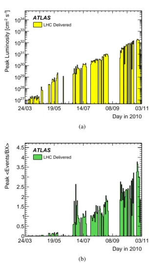
The maximum instantaneous luminosity per day is shown in Fig. 6(a). As luminosity increased and the trigger rates approached the limits imposed by offline processing,

Day in 2010

24/03 19/05 14/07 08/09 03/11

]-1 s-2 cmPeak Luminosity [

1027

1028

1029

1030

1031

1032

1033

1034 ^ATLAS LHC Delivered

(a)

Day in 2010

24/03 19/05 14/07 08/09 03/11

Peak <Events/BX>

0 0.5 1 1.5 2 2.5 3 3.5 4

4.5 ATLAS LHC Delivered

(b)

Fig. 6 Profiles with respect to time of (a) the maximum instantaneous luminosity per day and (b) the peak mean number of interactions per bunch crossing (assuming a total inelastic cross section of 71.5 mb) recorded by ATLAS during stable beams in √

s = 7 TeV pp collisions.

Both plots use the online luminosity measurement

primary and supporting triggers continued to evolve by pro-

gressively tightening the HLT selection cuts and by prescal-

ing the lower E _T threshold triggers. Table 5 shows the lowest

Rate [Hz]

10

10

10

JetTauEtmiss stream Muon stream Egamma stream

EF L2 L1

ATLAS

Online Prediction

s-1

cm-2

Luminosity = 1032

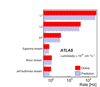
Fig. 7 Comparison of online rates (solid) with offline rate predictions (hashed) at luminosity 10

cm

s

for L1, L2, EF and main physics streams

unprescaled threshold of various trigger signatures for three luminosity values.

In order to prepare for higher luminosities, tools to op- timize prescale factors became very important. For exam- ple, the rate prediction tool uses enhanced bias data (data recorded with a very loose L1 trigger selection and no HLT selection) as input. Initially, these data were collected in dedicated enhanced bias runs using the lowest trigger thresh- olds, which were unprescaled at L1, and no HLT selec- tion. Subsequently, enhanced bias triggers were added to the physics menu to collect the data sample during normal physics data-taking.

Figure 7 shows a comparison between online rates at 10 ³² cm

s

and predictions based on extrapolation from enhanced bias data collected at lower luminosity. In gen- eral online rates agreed with predictions within 10%. The biggest discrepancy was seen in rates from the JetTauEt- miss stream, as a result of the non-linear scaling of E _T ^miss and

∑E T trigger rates with luminosity, as shown later in Fig. 13.

This non-linearity is due to in-time pile-up, defined as the effect of multiple pp interactions in a bunch crossing. The maximum mean number of interactions per bunch crossing, which reached 3.5 in 2010, is shown as a function of day in Fig. 6(b). In-time pile-up had the most significant effects on the E _T ^miss , ∑E T (Section 6.6), and minimum bias (Sec- tion 6.1) signatures. Out-of-time pile-up is defined as the ef- fect of an earlier bunch crossing on the detector signals for the current bunch crossing. Out-of-time pile-up did not have a significant effect in the 2010 pp data-taking because the bunch spacing was 150 ns or larger.

4 Level 1

The Level 1 (L1) trigger decision is formed by the Cen- tral Trigger Processor (CTP) based on information from the calorimeter trigger towers and dedicated triggering layers in the muon system. An overview of the CTP, L1 calorimeter, and L1 muon systems and their performance follows. The CTP also takes input from the MBTS, LUCID and ZDC sys- tems, described in Section 6.1.

4.1 Central Trigger Processor

The CTP [1, 8] forms the L1 trigger decision by applying the multiplicity requirements and prescale factors specified in the trigger menu to the inputs from the L1 trigger sys- tems. The CTP also provides random triggers and can apply specific LHC bunch crossing requirements. The L1 trigger decision is distributed, together with timing and control sig- nals, to all ATLAS sub-detector readout systems.

The timing signals are defined with respect to the LHC bunch crossings. A bunch crossing is defined as a 25 ns time- window centred on the instant at which a proton bunch may traverse the ATLAS interaction point. Not all bunch cross- ings contain protons; those that do are called filled bunches.

In 2010, the minimum spacing between filled bunches was 150 ns. In the nominal LHC configuration, there are a max- imum of 3564 bunch crossings per LHC revolution. Each bunch crossing is given a bunch crossing identifier (BCID) from 0 to 3563. A bunch group consists of a numbered list of BCIDs during which the CTP generates an internal trig- ger signal. The bunch groups are used to apply specific re- quirements to triggers such as paired (colliding) bunches for physics triggers, single (one-beam) bunches for back- ground triggers, and empty bunches for cosmic ray, noise and pedestal triggers.

4.1.1 Dead-time

Following an L1 accept the CTP introduces dead-time, by vetoing subsequent triggers, to protect front-end readout buffers from overflowing. This preventive dead-time mecha- nism limits the minimum time between two consecutive L1 accepts (simple dead-time), and restricts the number of L1 accepts allowed in a given period (complex dead-time). In 2010 running, the simple dead-time was set to 125 ns and the complex dead-time to 8 triggers in 80 µs. This preventa- tive dead-time is in addition to busy dead-time which can be introduced by ATLAS sub-detectors to temporarily throttle the trigger rate.

The CTP monitors the total L1 trigger rate and the rates

of individual L1 triggers. These rates are monitored before

and after prescales and after dead-time related vetoes have

been applied. One use of this information is to provide a

Day in 2010 01 Apr 01 May 31 May 30 Jun 30 Jul 29 Aug 28 Sep 28 Oct

L1 Live fraction [ % ]

20 30 40 50 60 70 80 90 100

110 ATLAS

Fig. 8 L1 live fraction per run throughout the full data-taking period of 2010, as used for luminosity estimates for correcting trigger dead-time effects. The live fraction is derived from the trigger L1 MBTS 2

measure of the L1 dead-time, which needs to be accounted for when determining the luminosity. The L1 dead-time cor- rection is determined from the live fraction, defined as the ratio of trigger rates after CTP vetoes to the corresponding trigger rates before vetoes. Figure 8 shows the live fraction based on the L1 MBTS 2 trigger (Section 6.1), the primary trigger used for these corrections in 2010. The bulk of the data were recorded with live fractions in excess of 98%. As a result of the relatively low L1 trigger rates and a bunch spacing that was relatively large (≥ 150 ns) compared to the nominal LHC spacing (25 ns), the preventive dead-time was typically below 10

and no bunch-to-bunch variations in dead-time existed.

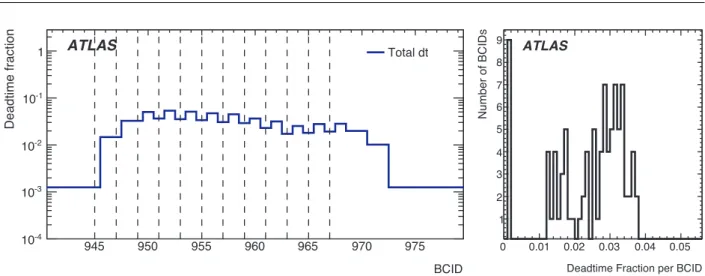
Towards the end of the 2010 data-taking a test was per- formed with a fill of bunch trains with 50 ns spacing, the running mode expected for the bulk of 2011 data-taking. The dead-time measured during this test is shown as a function of BCID in Fig. 9, taking a single bunch train as an exam- ple. The first bunch of the train (BCID 945) is only sub- ject to sub-detector dead-time of ∼0.1%, while the follow- ing bunches in the train (BCIDs 947 to 967) are subject to up to 4% dead-time as a result of the preventative dead-time generated by the CTP. The variation in dead-time between bunch crossings will be taken into account when calculating the dead-time corrections to luminosity in 2011 running.

4.1.2 Rates and Timing

Figure 10 shows the trigger rate for the whole data-taking period of 2010, compared to the luminosity evolution of the LHC. The individual rate points are the average L1 trigger rates in ATLAS runs with stable beams, and the luminosity points correspond to peak values for the run. The increasing

selectivity of the trigger during the course of 2010 is illus- trated by the fact that the L1 trigger rate increased by one order of magnitude; whereas, the peak instantaneous lumi- nosity increased by five orders of magnitude. The L1 trigger system was operated at a maximum trigger rate of just above 30 kHz, leaving more than a factor of two margin to the de- sign rate of 75 kHz.

The excellent level of synchronization of L1 trigger sig- nals in time is shown in Fig. 11 for a selection of L1 trig- gers. The plot represents a snapshot taken at the end of Oc- tober 2010. Proton-proton collisions in nominal filled paired bunch crossings are defined to occur in the central bin at 0.

As a result of mistiming caused by alignment of the calorime- ter pulses that are longer than a single bunch crossing, trig- ger signals may appear in bunch crossings preceding or suc- ceeding the central one. In all cases mistiming effects are below 10

. The timing alignment procedures for the L1 calorimeter and L1 muon triggers are described in Section 4.2 and Section 4.3 respectively.

4.2 L1 Calorimeter Trigger

The L1 calorimeter trigger [9] is based on inputs from the electromagnetic and hadronic calorimeters covering the re- gion |η| < 4.9. It provides triggers for localized objects (e.g.

electron/photon, tau and jet) and global transverse energy

triggers. The pipelined processing and logic is performed in

a series of custom built hardware modules with a latency of

less than 1 µs. The architecture, calibration and performance

of this hardware trigger are described in the following sub-

sections.

BCID

945 950 955 960 965 970 975

D e a d ti me f ra ct io n

10

10

10

10

1 ATLAS Total dt

Deadtime Fraction per BCID 0 0.01 0.02 0.03 0.04 0.05

Number of BCIDs

1 2 3 4 5 6 7 8

9

ATLAS

Fig. 9 L1 dead-time fractions per bunch crossing for a LHC test fill with a 50 ns bunch spacing. The dead-time fractions as a function of BCID (left), taking a single bunch train of 12 bunches as an example and a histogram of the individual dead-time fractions for each paired bunch crossing (right). The paired bunch crossings (odd-numbered BCID from 945 to 967) are indicated by vertical dashed lines on the left hand plot

01 Apr 01 May 31 May 30 Jun 30 Jul 29 Aug 28 Sep 28 Oct

-1-230Luminosity [10 cm s ] ^-310

10-2 10-1 1 10

102 _ATLAS

Day in 2010 01 Apr 01 May 31 May 30 Jun 30 Jul 29 Aug 28 Sep 28 Oct L1 Trigger Rate [Hz] 3

10 104

Fig. 10 Evolution of the L1 trigger rate throughout 2010 (lower panel), compared to the instantaneous luminosity evolution (upper panel)

Relative Timing [ bunch crossing ]

-3 -2 -1 0 1 2 3

Fraction of L1 trigger signals

10-6

10-5

10-4

10-3

10-2

10-1

1 _TAU6

EM10 J15 FJ10

ATLAS

Fig. 11 L1 trigger signals in units of bunch crossings for a number of triggers. The trigger signal time is plotted relative to the position of filled paired bunches for a particular data-taking period towards the end of the 2010 pp run

4.2.1 L1 Calorimeter Trigger Architecture

The L1 calorimeter trigger decision is based on dedicated analogue trigger signals provided by the ATLAS calorime- ters independently from the signals read out and used at the HLT and offline. Rather than using the full granularity of the calorimeter, the L1 decision is based on the information from analogue sums of calorimeter elements within projec- tive regions, called trigger towers. The trigger towers have a size of approximately ∆ η × ∆ φ = 0.1 × 0.1 in the cen- tral part of the calorimeter, |η| < 2.5, and are larger and less regular in the more forward region. Electromagnetic and hadronic calorimeters have separate trigger towers.

The 7168 analogue inputs must first be digitized and

then associated to a particular LHC bunch crossing. Much

of the tuning of the timing and transverse energy calibra-

tion was performed during the 2010 data-taking period since

the final adjustments could only be determined with collid-

ing beam events. Once digital transverse energies per LHC

bunch crossing are formed, two separate processor systems,

working in parallel, run the trigger algorithms. One system, the cluster processor uses the full L1 trigger granularity in- formation in the central region to look for small localized clusters typical of electron, photon or tau particles. The other, the jet and energy-sum processor, uses 2 × 2 sums of trig- ger towers, called jet elements, to identify jet candidates and form global transverse energy sums: missing transverse en- ergy, total transverse energy and jet-sum transverse energy.

The magnitude of the objects and sums are compared to programmable thresholds to form the trigger decision. The thresholds used in 2010 are shown in Table 1 in Section 2.

Vertical sums

!

! Horizontal sums

! !

!

!

Electromagnetic isolation ring Hadronic inner core and isolation ring

Electromagnetic calorimeter

Hadronic calorimeter

Trigger towers ("# × "$= 0.1 × 0.1)

Local maximum/

Region-of-interest

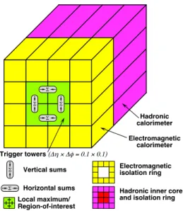
Fig. 12 Building blocks of the electron/photon and tau algorithms with the sums to be compared to programmable thresholds

The details of the algorithms can be found elsewhere [9]

and only the basic elements are described here. Figure 12 il- lustrates the electron/photon and tau triggers as an example.

The electron/photon trigger algorithm identifies an Region of Interest as a 2 × 2 trigger tower cluster in the electro- magnetic calorimeter for which the transverse energy sum from at least one of the four possible pairs of nearest neigh- bour towers (1 ×2 or 2 ×1) exceeds a pre-defined threshold.

Isolation-veto thresholds can be set for the 12-tower sur- rounding ring in the electromagnetic calorimeter, as well as for hadronic tower sums in a central 2 × 2 core behind the cluster and the 12-tower hadronic ring around it. Isolation requirements were not applied in 2010 running. Jet RoIs are defined as 4 × 4, 6 × 6 or 8 × 8 trigger tower windows for which the summed electromagnetic and hadronic transverse energy exceeds pre-defined thresholds and which surround a 2 × 2 trigger tower core that is a local maximum. The lo- cation of this local maximum also defines the coordinates of the jet RoI.

The real-time output to the CTP consists of more than 100 bits per bunch crossing, comprising the coordinates and threshold bits for each of the RoIs and the counts of the num-

ber of objects (saturating at seven) that satisfy each of the electron/photon, tau and jet criteria.

4.2.2 L1 Calorimeter Trigger Commissioning and Rates After commissioning with cosmic ray and collision data, in- cluding event-by-event checking of L1 trigger results against offline emulation of the L1 trigger logic, the calorimeter trig- ger processor ran stably and without any algorithmic errors.

Bit-error rates in digital links were less than 1 in 10 ²⁰ . Eight out of 7168 trigger towers were non-operational in 2010 due to failures in inaccessible analogue electronics on the detec- tor. Problems with detector high and low voltage led to an additional ∼1% of trigger towers with low or no response.

After calibration adjustments, L1 calorimeter trigger condi- tions remained essentially unchanged for 99% of the 2010 proton-proton integrated luminosity.

-1]

-2s

30cm

bunch [10 Luminosity / N

0.2 0.25 0.3 0.35 0.4

[Hz]bunchL1 rate / N

0 10 20 30 40 50 60 70 80

J10 EM5 TAU5

TE100 XE10

×0.2) (

-1]

-2s

30cm

bunch [10 Luminosity / N

0.2 0.25 0.3 0.35 0.4

[Hz]bunchL1 rate / N

0 10 20 30 40 50 60 70 80

ATLAS

Fig. 13 L1 trigger rate scaling for some low threshold trigger items as a function of luminosity per bunch crossing. The rate for XE10 has been scaled by 0.2

The scaling of the L1 trigger rates with luminosity is shown in Fig. 13 for some of the low-threshold calorimeter trigger items. The localised objects, such as electrons and jet candidates, show an excellent linear scaling relationship with luminosity over a wide range of luminosities and time.

Global quantities such as the missing transverse energy and total transverse energy triggers also scale in a smooth way, but are not linear as they are strongly affected by in-time pile-up which was present in the later running periods.

4.2.3 L1 Calorimeter Trigger Calibration

In order to assign the calorimeter tower signals to the cor-

rect bunch crossing, a task performed by the bunch cross-

ing identification logic, the signals must be synchronized to

the LHC clock phase with nanosecond precision. The tim-

ing synchronization was first established with calorimeter

pulser systems and cosmic ray data and then refined using

the first beam delivered to the detector in the splash events (Section 3). During the earliest data-taking in 2010 the cor- rect bunch crossing was determined for events with trans- verse energy above about 5 GeV. Timing was incrementally improved, and for the majority of the 2010 data the timing of most towers was better than ±2 ns, providing close to ideal performance.

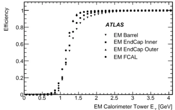
In order to remove the majority of fake triggers due to small energy deposits, signals are processed by an optimized filter and a noise cut of around 1.2 GeV is applied to the trigger tower energy. The efficiency for an electromagnetic tower energy to be associated to the correct bunch crossing and pass this noise cut is shown in Fig. 14 as a function of the sum of raw cell E _T within that tower, for different regions of the electromagnetic calorimeter. The efficiency turn-on is consistent with the optimal performance expected from a simulation of the signals and the full efficiency in the plateau region indicates the successful association of these small energy deposits to the correct bunch crossing.

Special treatment, using additional bunch crossing iden- tification logic, is needed for saturated pulses with E _T above about 250 GeV. It was shown that BCID logic performance was more than adequate for 2010 LHC energies, working for most trigger towers up to transverse energies of 3.5 TeV and beyond. Further tuning of timing and algorithm parameters will ensure that the full LHC energy range is covered.

[GeV]

EM Calorimeter Tower ET

0 0.5 1 1.5 2 2.5 3 3.5 4

Efficiency

0 0.2 0.4 0.6 0.8 1

EM Barrel EM EndCap Inner EM EndCap Outer EM FCAL ATLAS

Fig. 14 Efficiency for an electromagnetic trigger tower energy to be as- sociated with the correct bunch crossing and pass a noise cut of around 1.2 GeVas a function of the sum of raw cell E

within that tower

In order to obtain the most precise transverse energy measurements, a transverse energy calibration must be ap- plied to all trigger towers. The initial transverse energy calibration was produced by calibration pulser runs. In these runs signals of a controlled size are injected into the calorimeters. Subsequently, with sufficient data, the gains were recalibrated by comparing the transverse ener- gies from the trigger with those calculated offline from the full calorimeter information. By the end of the 2010 data- taking this analysis had been extended to provide a more

1 10 102

[GeV]

Offline ET

0 10 20 30 40 50

TL1 E [GeV]

0 10 20 30 40

50 ATLAS

(a)

1 10 102

[GeV]

Offline ET

0 10 20 30 40 50

TL1 E [GeV]

0 10 20 30 40

50 ATLAS

(b)

Fig. 15 Typical transverse energy correlation plots for two individual central calorimeter towers, (a) electromagnetic and (b) hadronic

precise calibration on a tower-by-tower basis. In most cases, the transverse energies derived from the updated calibration differed by less than 3% from those obtained from the orig- inal pulser-run based calibration. Examples of correlation plots between trigger and offline calorimeter transverse en- ergies can be seen in Fig. 15. In the future, with even larger datasets, the tower-by-tower calibration will be further re- fined based on physics objects with precisely known ener- gies, for example, electrons from Z boson decays.

4.3 L1 Muon Trigger

The L1 muon trigger system [1],[10] is a hardware-based

system to process input data from fast muon trigger detec-

tors. The system’s main task is to select muon candidates

and identify the bunch crossing in which they were pro-

duced. The primary performance requirement is to be effi-

cient for muon p _T thresholds above 6 GeV. A brief overview

of the L1 muon trigger is given here; the performance of the

muon trigger is presented in Section 6.3.

Fig. 16 A section view of the L1 muon trigger chambers. TCG I was not used in the trigger in 2010

4.3.1 L1 Muon Trigger Architecture

Muons are triggered at L1 using the RPC system in the bar- rel region (|η| < 1.05) and the TGC system in the end-cap regions (1.05 < |η| < 2.4), as shown in Fig. 16. The RPC and TGC systems provide rough measurements of muon can- didate p _T , η , and φ. The trigger chambers are arranged in three planes in the barrel and three in each endcap (TCG I shown in Fig. 16 did not participate in the 2010 trigger).

Each plane is composed of two to four layers. Muon can- didates are identified by forming coincidences between the muon planes. The geometrical coverage of the trigger in the end-caps is ≈ 99%. In the barrel the coverage is reduced to

≈ 80% due to a crack around η = 0, the feet and rib support structures for the ATLAS detector and two small elevators in the bottom part of the spectrometer.

The L1 muon trigger logic is implemented in similar ways for both the RPC and TCG systems, but with the fol- lowing differences:

– The planes of the RPC system each consist of a doublet of independent detector layers, each read out in the η (z) and φ coordinates. A low-p _T trigger is generated by requiring a coincidence of hits in at least 3 of the 4 layers of the inner two planes, labelled as RPC1 and RPC2 in Fig. 16). The high-p T logic starts from a low-p T trigger, then looks for hits in one of the two layers of the high-p _T confirmation plane (RPC3).

– The two outermost planes of the TGC system (TGC2 and TGC3) each consist of a doublet of independent de- tectors read out by strips to measure the φ coordinate and wires to measure the η coordinate. A low- p T trigger is generated by a coincidence of hits in at least 3 of the 4 layers of the outer two planes. The inner plane (TGC1) contains 3 detector layers, the wires are read out from all of these, but the strips from only 2 of the layers. The high-p _T trigger requires at least one of two φ -strip layers

and 2 out of 3 wire layers from the innermost plane in coincidence with the low- p _T trigger.

In both the RPC and TGC systems, coincidences are gener- ated separately for η and φ and can then be combined with programmable logic to form the final trigger result. The con- figuration for the 2010 data-taking period required a logical AND between the η and φ coincidences in order to have a muon trigger.

In order to form coincidences, hits are required to lie within parametrized geometrical muon roads. A road repre- sents an envelope containing the trajectories, from the nom- inal interaction point, of muons of either charge with a p T

above a given threshold. Example roads are shown in Fig. 16.

There are six programmable p _T thresholds at L1 (see Ta- ble 1) which are divided into two sets: three low-p _T thresh- olds to cover values up to 10 GeV, and three high-p _T thresh- olds to cover p _T greater than 10 GeV.

To enable the commissioning and validation of the per- formance of the system for 2010 running, two triggers were defined which did not require coincidences within roads and thus gave maximum acceptance and minimum trigger bias.

One (MU0) based on low-p _T logic and the other (MU0 COMM) based on the high-p _T logic. For these trig- gers the only requirement was that hits were in the same trigger tower (η × φ ∼ 0.1 × 0.1).

[BC]

- Time

Time

-3 -2 -1 0 1 2 3 4 5

Fraction of signals

0 0.2 0.4 0.6 0.8 1

1.2 ATLAS

TGC

RPC after calibration RPC before calibration

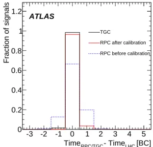
Fig. 17 The timing alignment with respect to the LHC bunch clock (25 ns units) for the RPC system (before and after the timing calibra- tion) and the TGC system

4.3.2 L1 Muon Trigger Timing Calibration

In order to assign the hit information to the correct bunch

crossing, a precise alignment of RPC and TGC signals, or

timing calibration, was performed to take into account signal delays in all components of the read out and trigger chain.

Test pulses were used to calibrate the TGC timing to within 25 ns (one bunch crossing) before the start of data-taking.

Tracks from cosmic ray and collision data were used to cal- ibrate the timing of the RPC system. This calibration re- quired a sizable data sample to be collected before a time alignment of better than 25 ns was reached. As described in section 4.1, the CTP imposes a 25 ns window about the nom- inal bunch crossing time during which signals must arrive in order to contribute to the trigger decision. In the first phase of the data-taking, while the timing calibration of the RPC system was on-going, a special CTP configuration was used to increase the window for muon triggers to 75 ns. The ma- jority of 2010 data were collected with both systems aligned to within one bunch crossing for both high-p _T and low-p _T triggers. In Fig. 17 the timing alignment of the RPC and TGC systems is shown with respect to the LHC bunch clock in units of the 25 ns bunch crossings (BC).

5 High Level Trigger Reconstruction

The HLT has additional information available, compared to L1, including inner detector hits, full information from the calorimeter and data from the precision muon detectors. The HLT trigger selection is based on features reconstructed in these systems. The reconstruction is performed, for the most part, inside RoIs in order to minimize execution times and reduce data requests across the network at L2. The sections below give a brief description of the algorithms for inner detector tracking, beamspot measurement, calorimeter clus- tering and muon reconstruction. The performance of the al- gorithms is presented, including measurements of execution times which meet the timing constraints outlined in Sec- tion 2.

5.1 Inner Detector Tracking

The track reconstruction in the Inner Detector is an essen- tial component of the trigger decision in the HLT. A robust and efficient reconstruction of particle trajectories is a pre- requisite for triggering on electrons, muons, B-physics, taus, and b-jets. It is also used for triggering on inclusive pp in- teractions and for the online determination of the beamspot (Section 5.2), where the reconstructed tracks provide the in- put to reconstruction of vertices. This section gives a short description of the reconstruction algorithms and an overview of the performance of the track reconstruction with a focus on tracking efficiencies in the ATLAS trigger system.

5.1.1 Inner Detector Tracking Algorithms

The L2 reconstruction algorithms are specifically designed to meet the strict timing requirements for event processing at L2. The track reconstruction at the EF is less time con- strained and can use, to a large extent, software components from the offline reconstruction. In both L2 and EF the track finding is preceded by a data preparation step in which de- tector data are decoded and transformed to a set of hit po- sitions in the ATLAS coordinate system. Clusters are first formed from adjacent signals on the SCT strips or in the Pixel detector. Two-dimensional Pixel clusters and pairs of one-dimensional SCT clusters (from back-to-back detectors rotated by a small stereo angle with respect to one another) are combined with geometrical information to provide three- dimensional hit information, called space-points. Clusters and space-points provide the input to the HLT pattern recog- nition algorithms.

The primary track reconstruction strategy is inside-out tracking which starts with pattern recognition in the SCT and Pixel detectors; track candidates are then extended to the TRT volume. In addition, the L2 has an algorithm that reconstructs tracks in the TRT only and the EF has an addi- tional track reconstruction strategy that is outside-in, starting from the TRT and extending the tracks to the SCT and Pixel detectors.

Track reconstruction at both L2 and EF is run in an RoI- based mode for electron, muon, tau and b-jet signatures. B- physics signatures are based either on a FullScan (FS) mode (using the entire volume of the Inner Detector) or a large RoI. The tracking algorithms can be configured differently for each signature in order to provide the best performance.

L2 uses two different pattern recognition strategies:

– A three-step histogramming technique, called IdScan.

First, the z-position of the primary vertex, z

, is deter- mined as follows. The RoI is divided into φ-slices and z-intercept values are calculated and histogrammed for lines through all possible pairs of space-points in each phi-slice; z

is determined from peaks in this histogram.

The second step is to fill a (η, φ) histogram with val-

ues calculated with respect to z

for each space-point

in the RoI; groups of space-points to be passed on to

the third step are identified from histogram bins con-

taining at least four space-points from different detec-

tor layers. In the third step, a (1/p _T , φ ) histogram is

filled from values calculated for all possible triplets of

space-points from different detector layers; track can-

didates are formed from bins containing at least four

space-points from different layers. This technique is the

approach used for electron, muon and B-physics triggers

due to the slightly higher efficiency of IdScan relative to

SiTrack.

[GeV]

Track pT

10 10²

Efficiency

0.7 0.75 0.8 0.85 0.9 0.95 1

ATLAS

L2 EF

(a)

[GeV]

Track pT

10 10²

Efficiency

0.7 0.75 0.8 0.85 0.9 0.95 1

ATLAS

L2 EF

(b)

Fig. 18 L2 and EF tracking reconstruction efficiency with respect to offline (a) muon candidates and (b) electron candidates

[GeV]

Track p

103 10⁴

Ef fi ci e n cy

0 0.5 1.0

L2 EF

10-1 1 10

ATLAS

(a)

[GeV]

Track p

103 10⁴

Ef fi ci e n cy

0 0.5 1.0

L2 EF

10-1 1 10

ATLAS

(b)

Fig. 19 L2 and EF tracking reconstruction efficiency with respect to offline reference tracks inside (a) tau RoIs and (b) jet RoIs

– A combinatorial technique, called SiTrack. First, pairs of hits consistent with a beamline constraint are found within a subset of the inner detector layers. Next, triplets are formed by associating additional hits in the remain- ing detector layers consistent with a track from the beam- line. In the final step, triplets consistent with the same track trajectory are merged, duplicate or outlying hits are removed and the remaining hits are passed to the track fitter. SiTrack is the approach used for tau and jet triggers as well as the beamspot measurement as it has a slightly lower fake-track fraction.

In both cases, track candidates are further processed by a common Kalman [11] filter track fitter and extended to the TRT for an improved p _T resolution and to benefit from the electron identification capability of the TRT.

The EF track reconstruction is based on software shared with the offline reconstruction [12]. The offline software was extended to run in the trigger environment by adding sup- port for reconstruction in an RoI-based mode. The pattern recognition in the EF starts from seeds built from triplets of

space-points in the Pixel and SCT detectors. Triplets consist of space-points from different layers, all in the pixel detec- tor, all in the the SCT or two space-points in the pixel detec- tor and one in the SCT. Seeds are preselected by imposing a minimum requirement on the momentum and a maximum requirement on the impact parameters. The seeds define a road in which a track candidate can be formed by adding additional clusters using a combinatorial Kalman filter tech- nique. In a subsequent step, the quality of the track candi- dates is evaluated and low quality candidates are rejected.

The tracks are then extended into the TRT and a final fit is performed to extract the track parameters.

5.1.2 Inner Detector Tracking Algorithms Performance

The efficiency of the tracking algorithms is studied using

specific monitoring triggers, which do not require a track

to be present for the event to be accepted, and are thus

unbiased for track efficiency measurements. The efficiency

is defined as the fraction of offline reference tracks that

are matched to a trigger track (with matching requirement

η

-3 -2 -1 0 1 2 3

]-1 [GeV95RMS

0 0.001 0.002 0.003 0.004 0.005 0.006 0.007

ATLAS

L2 EF

Fig. 20 The RMS of the core 95% (RMS

) of the inverse-p

residual as a function of offline track η

∆ R = p

∆ φ ² + ∆ η ² < 0.1). Offline reference tracks are re- quired to have |η| < 2.5, |d ₀ | < 1.5 mm, |z ₀ | < 200 mm and

|(z ₀ −z

)sin θ | < 1.5 mm, where d ₀ and z ₀ are the transverse and longitudinal impact parameters, and z

is the position of the primary vertex along the beamline as reconstructed of- fline. The reference tracks are also required to have one Pixel hit and at least six SCT clusters. For tau and jet RoIs, the ref- erence tracks are additionally required to have χ ² probabil- ity of the track fit higher than 1%, two Pixel hits, one in the innermost layer, and a total of at least seven SCT clusters.

The L2 and EF tracking efficiencies are shown as a func- tion of p _T for offline muon candidates in Fig. 18(a) and for offline electron candidates in Fig. 18(b). Tracking efficien- cies in tau and jet RoIs are shown in Fig. 19, determined with respect to all offline reference tracks lying within the RoI. In all cases, the efficiency is close to 100% in the p _T range important for triggering.

The RMS of the core 95% (RMS ₉₅ ) of the inverse-p _T residual (( ¹

pT

) ^trigger − ( ¹

pT

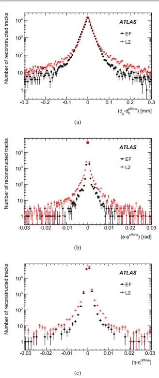
) ^offline ) distribution is shown as a function of η in Fig. 20. Both L2 and EF show good agree- ment with offline, although the residuals between L2 and offline are larger, particularly at high |η| as a consequence of the speed-optimizations made at L2. Figure 21 shows the residuals in d ₀ , φ and η . Since it uses offline software, EF tracking performance is close to that of the offline re- construction. Performance is not identical, however, due to an online-specific configuration of offline software designed to increase speed and be more robust to compensate for the more limited calibration and detector status information available in the online environment.

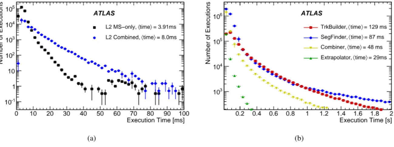
5.1.3 Inner Detector Tracking Algorithms Timing

Distributions of the algorithm execution time at L2 and EF are shown in Fig. 22. The total time for L2 reconstruction is shown in Fig. 22(a) for a muon algorithm in RoI and FullScan mode. The times of the different reconstruction steps at the EF are shown in Fig. 22(b) for muon RoIs and

) [mm]

offline

-d0

(d0

-0.3 -0.2 -0.1 0 0.1 0.2 0.3

Number of reconstructed tracks

1 10 102

103

104 ATLAS

EF L2

(a)

) [rad]

offline

φ φ- (

-0.03 -0.02 -0.01 0 0.01 0.02 0.03

Number of reconstructed tracks

1 10 102

103

104

ATLAS EF L2

(b)

offline) η η- ( -0.03 -0.02 -0.01 0 0.01 0.02 0.03

Number of reconstructed tracks

1 10 102

103

104

ATLAS EF L2

(c)

Fig. 21 Residuals with respect to offline for track parameters (a) d

, (b) φ and (c) η

in Fig. 22(c) for FullScan mode. The execution times are

shown for all instances of the algorithm execution, whether

the trigger was passed or not. The execution times are well

within the online constraints.