A TLAS-CONF-2017-061 13 July 2017
ATLAS CONF Note
ATLAS-CONF-2017-061
The ATLAS Tau Trigger in Run 2
The ATLAS Collaboration
12th July 2017
This note describes the algorithms and selections used in the ATLAS experiment to trigger on hadronically decaying tau leptons in the LHC Run 2. The performance of the tau trigger in the 33 fb − 1 of pp collision data recorded in 2016 at
√ s = 13 TeV is documented.
© 2017 CERN for the benefit of the ATLAS Collaboration.
Reproduction of this article or parts of it is allowed as specified in the CC-BY-4.0 license.
1 Introduction
Tau leptons are a key signature for many measurements of Standard Model (SM) processes and for searches for new physics at the LHC [1]. The decay into tau lepton pairs provides the strongest signal for measurements of the SM Higgs boson coupling to fermions [2]. Final states containing tau leptons are also often favoured by heavier Higgs bosons or other new resonances in many scenarios beyond the SM [3–5].
Most of these analyses rely on triggering exclusively on hadronically decaying tau leptons. Achieving high acceptance for such hadronic signatures within the bandwidth and computing constraints of the trigger system is very challenging at the LHC.
With a mass of 1776 . 86 ± 0 . 12 MeV and a proper decay length of 87 . 03 ± 0 . 15 µ m [6], tau leptons decay either leptonically ( τ → `ν ` ν τ , ` = e, µ ) or hadronically ( τ → hadrons ν τ ) and do so typically before reaching active regions of the ATLAS detector [7]. The hadronic decays represent 65% of all possible tau lepton decay modes [6] and their decay products are typically one (“1-prong” decay) or three (“3-prong”
decay) charged pions and zero or one neutral pions. The neutral and charged hadrons stemming from the tau lepton decay make up the visible decay products of the tau lepton, and are in the following referred to as τ had-vis .
This note describes the tau trigger used in ATLAS to select events with hadronically decaying tau leptons in the pp collisions at the centre-of-mass energy
√ s = 13 TeV at the LHC. Dedicated tau trigger algorithms were designed and implemented based on the main features of hadronic tau decays: narrow calorimeter energy deposits and a small number of associated tracks. Due to the high production rate of jets with features similar to hadronic tau decays, keeping the rate of tau triggers under control is challenging. Compared to the LHC Run 1, this is even more challenging in the LHC Run 2 because of the higher production rate of jets from the increase in collision energy, the higher number of collisions per bunch-crossing (pile-up) and the reduced bunch spacing.
The performance of the tau trigger documented in this note is based on 33 fb − 1 of data collected in pp collisions recorded in 2016 at
√ s = 13 TeV. This dataset has been collected with a peak instantaneous luminosity of 1 . 37 × 10 34 cm − 2 s − 1 (1.37 times the LHC design) and a peak average number of interactions per bunch-crossing of 51.
This note is organised as follows. After a brief overview of the ATLAS trigger system in Section 2, the tau trigger algorithms and selections are detailed in Section 3. Section 4 describes the tau triggers implemented in 2016, together with preliminary results on the commissioning of the triggers using L1Topo. Section 5 shows the performance and efficiency of the tau trigger as measured in the 2016 data and Section 6 gives a summary of the presented material in this note.
2 The ATLAS trigger system in Run 2
The ATLAS Trigger and Data Acquisition (TDAQ) system used during the LHC Run 1 is detailed in
Refs. [8, 9] and the changes deployed for the LHC Run 2 are described in Ref. [10]. In the LHC Run 2, the
TDAQ system consists of a hardware-based first level trigger (L1) and a software-based high-level trigger (HLT). The maximum L1 accept rate is 100 kHz, while the average HLT physics output rate is 1000 Hz.
At L1, a new FPGA-based topological trigger (L1Topo) has been added and commissioned in 2016.
The L1Topo modules allow for geometric and kinematic selections on the L1 trigger objects. The L1 calorimeter trigger (L1Calo) [11] has been improved to better cope with the increase in rate in Run 2. These improvements include dynamic, bunch-by-bunch pedestal corrections, the measurement of the energy of electron, photon and tau objects in multiples of 0.5 GeV instead of 1 GeV, and the implementation of energy-dependent isolation criteria.
At the HLT, the merging of the two software-based trigger levels used in the LHC Run 1 improves the usage of CPU resources and removes the bandwidth limitation between the two levels. The HLT calorimeter reconstruction has access to the full detector granularity and is harmonised with the offline reconstruction.
Thanks to the optimisation of the data preparation and offline clustering algorithms, the topo-clustering algorithm [12] is fast enough to be executed on all events accepted by the L1 tau triggers. In 2016, bunch- by-bunch cell corrections [13] have been deployed to mitigate out-of-time pile-up effects and to improve the HLT energy resolution with respect to offline. The HLT tracking algorithms have also been improved and have integrated the information from the insertable B-layer (IBL) [14]. The tracking trigger is subdivided into fast tracking , based on trigger-specific pattern recognition algorithms, and precision tracking , based on offline tracking algorithms. These algorithms run inside the Regions-of-Interest (RoI) identified at L1 and the tracks found by the fast tracking are used to seed the precision tracking to reduce CPU usage.
3 Tau trigger algorithms and selections
All the new features of the ATLAS trigger system are extensively used by the tau trigger to cope with the significant increase in trigger rate and per-event processing CPU usage due to the higher instantaneous luminosity and higher pile-up in the LHC Run 2. A detailed description of the tau trigger used in the LHC Run 1 is given in Ref. [15].
3.1 Level-1 tau trigger
The L1 algorithm for the reconstruction of the τ had-vis candidate is the same as the one used in Run 1 [8, 15]
and it is based on calorimeter information. In the L1Calo trigger, two regions are defined for each candidate, using trigger towers in both the electromagnetic (EM) and hadronic (HAD) calorimeters: the core region, and the isolation region around this core. The trigger towers have a granularity of ∆η × ∆φ = 0 . 1 × 0 . 1 with a coverage of |η| < 2 . 5. The core region is defined as a square of 2 × 2 trigger towers, corresponding to 0 . 2 × 0 . 2 in ∆η × ∆φ space. The E T of a τ had-vis candidate at L1 is taken as the sum of the transverse energy in the two most energetic neighbouring central towers in the EM calorimeter core region, and in the 2 × 2 towers in the HAD calorimeter, all calibrated at the EM scale. For each τ had-vis candidate, the EM isolation E EM isol
T is calculated as the transverse energy deposited in the annulus between 0 . 2 × 0 . 2 and 0 . 4 × 0 . 4 in
the EM calorimeter.
To suppress background events and thus reduce trigger rates, a new energy-dependent upper threshold on the EM isolation energy E EM isol
T [GeV] ≤ (E T [GeV] / 10 + 2 ) is applied for τ had-vis candidates up to 60 GeV.
This requirement has been tuned with
√ s = 13 TeV simulation to yield a selection efficiency of 98% and it is an improved selection with respect to what was used in Run 1, when an upper threshold of E EM isol
T < 4 GeV was applied at any transverse energy of the τ had-vis candidate. Above 60 GeV, no isolation requirement is applied.
The energy resolution at L1 is significantly worse than in the offline reconstruction. This is due to the fact that all cells in a trigger tower are combined without the use of sophisticated clustering algorithms and without τ had-vis -specific energy calibrations. Also, the coarse energy and geometrical position granularity limits the precision of the measurement. These effects lead to a significant signal efficiency loss for low- E T τ had-vis candidates.
In case of combined τ + e/µ/τ triggers, further reductions in rate are achieved by means of additional kinematic and geometric selections implemented at L1Topo. The algorithms used in the tau triggers are based on the angular selection ∆R = p
(∆φ) 2 + (∆η) 2 applied to the L1 objects above given E T thresholds contained in the lists of L1 objects provided by L1Calo. This selection is either applied to find τ + e/µ/τ pairs with objects that are not back-to-back ( ∆R < 2 . 9) or to find jet candidates not overlapping ( ∆R > 0 . 1) with the τ had-vis candidate (or the electron candidate in case of τ + e triggers). These selections are driven by the event topologies of the target final states and are motivated in Section 4. The L1Topo hardware has been deployed in 2016. Among the L1Topo algorithms used in the tau triggers, only those with the 2 τ selection have been commissioned (see Section 4.1) and used for physics in the last part of the 2016 pp data taking period. The commissioning of the remaining algorithms will be completed in 2017.
3.2 HLT tau trigger
The HLT tau trigger is subdivided in three steps: calo-only preselection , track preselection and offline-like selection . At each step, a different τ had-vis reconstruction is executed and a selection is applied to reduce the rate of the τ had-vis candidates processed in the following steps. The less CPU expensive algorithms are executed at the beginning of the HLT, while the more CPU intensive ones, like the precision tracking, are executed in the last step and only on the candidates passing the previous selections.
3.2.1 Calo-only preselection
At the first stage, the τ had-vis candidate is reconstructed as in Run 1 [15], but purely from calorimeter information. Calorimeter cells inside the RoI identified at L1 are retrieved and the topo-clustering algorithm is executed. Thanks to the full detector granularity and the bunch-by-bunch pile-up corrections, the energies of these reconstructed topo-clusters are very close to the offline ones. These clusters are calibrated with the local hadron calibration (LC) [16] and their vectorial sum is used as a ‘jet seed’ for the reconstruction of the τ had-vis candidate. The energy of the τ had-vis candidate is calculated from the LC clusters in a cone of
∆R < 0 . 2 around the barycentre of the jet seed. A dedicated τ had-vis energy calibration (TES) is applied to
improve the precision of the energy measurement and follows the offline procedure [15]. This calibration
is derived from simulation as a function of the p T and pseudorapidity of the τ had-vis candidate and includes
pile-up corrections. There are two noticeable differences in this procedure from the one used offline. The pile-up corrections are parameterised as a function of the average number of interactions per bunch-crossing ( µ ) as measured online. Both the online and offline µ values are measured using the LUCID detector, but the online value is determined using a preliminary calibration available at the time the data were recorded [17]. Moreover, the online value is not updated for each luminosity block (the basic time unit for storing ATLAS luminosity information for physics) as in the offline reconstruction, but only when the instantaneous luminosity varies by more than 5%. That means that on average the pile-up corrections are based on an online µ value slightly higher than the actual one. The second difference is that the TES is not parametrised as a function of the τ had-vis candidate track multiplicity since at this stage the track information is not available. An inclusive TES is instead used.
After the calo-only τ had-vis reconstruction, a selection on the minimum p T of the τ had-vis candidate is applied and only the remaining candidates pass to the next stage of the HLT tau trigger.
3.2.2 Track preselection
In the second step of the HLT tau trigger, the track information is added to the τ had-vis reconstruction using the two-stage fast tracking [10] approach. This is a trigger-specific pattern recognition algorithm that runs in two stages. In the first stage, the leading track is sought in a narrow ∆R cone around the τ had-vis candidate along the entire beamline. In the second stage, additional tracks associated to the τ had-vis candidate are fit in a larger ∆R cone but in a narrow range around the leading track along the beamline. This strategy is CPU-efficient as it minimises the volume in which the pattern recognition algorithm is executed.
In more details, the fast tracking is executed in an RoI centred on the barycentre of the τ had-vis jet seed. In the first stage, a leading track with p T > 1 GeV is sought in a narrow cone of ∆R < 0 . 1 around the RoI centre and along the beamline in the range | z| < 225 mm. If no track is found, the τ had-vis is rejected. In the second stage, the fast tracking is executed in a wider cone of ∆R < 0 . 4 around the RoI centre, but only in the range |∆z | < 10 mm with respect to the leading track. Given that the τ had-vis z-position at the beamline is not known, without this two-staged approach it would be too CPU expensive to run the fast tracking in the RoI over the full beamline with the wider η and φ size of the RoI. The configuration of the two-stage fast tracking algorithm in terms of track minimum transverse momentum and RoI size has been optimised to yield the highest tracking efficiency within the available CPU resources. After the two-stage fast tracking, tracks with p T > 1 GeV are associated to the τ had-vis candidate as in the offline reconstruction [15]. The N trk
core core and N trk
isol isolation track multiplicities are computed based on the number of tracks found in ∆R < 0 . 2 and 0 . 2 < ∆R < 0 . 4 around the τ had-vis direction, respectively.
Only the τ had-vis candidates with 1 ≤ N core trk ≤ 3 and N trk
isol ≤ 1 pass to the final step of the HLT tau trigger.
These track multiplicity requirements achieve enough rate reduction to run more CPU intensive algorithms
on the accepted events, while keeping high efficiency for real τ had-vis .
3.2.3 Offline-like selection
The final stage of the HLT tau trigger consists of a more precise measurement of the tracks associated to the τ had-vis candidate and the application of the τ had-vis identification based on a Boosted Decision Tree (BDT) algorithm. This stage is executed only on the candidates passing the preselection stage described in the previous section.
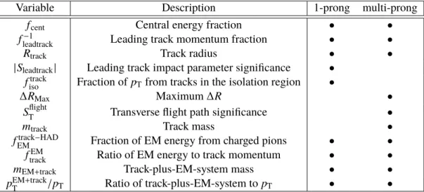
A precision-tracking algorithm similar to the offline one is run using tracks identified by the second step of the fast tracking as seeds to measure their properties more precisely. Using those tracks as well as the calorimeter information, the input variables for the τ had-vis identification are computed. Two sets of variables for 1-prong and multi-prong τ had-vis candidates are used depending on whether the number of precision tracks associated to the τ had-vis in ∆R < 0 . 2 is one or more than one, respectively. The implementation of these variables follows closely their offline counterparts, as described in Ref. [18]. The list of variables is described in Table 1. The only significant difference in the calculation of these variables between online
Variable Description 1-prong multi-prong
f cent Central energy fraction • •
f − 1
leadtrack Leading track momentum fraction • •
R track Track radius • •
| S leadtrack | Leading track impact parameter significance • f track
iso Fraction of p T from tracks in the isolation region •
∆R Max Maximum ∆R •
S flight
T Transverse flight path significance •
m track Track mass •
f track − HAD
EM Fraction of EM energy from charged pions • •
f EM
track Ratio of EM energy to track momentum • •
m EM+track Track-plus-EM-system mass • •
p EM+track
T /p T Ratio of track-plus-EM-system to p T • •
Table 1: Discriminating variables used as input to the tau identification algorithm for 1-prong and multi-prong τ had-vis candidates.
and offline is for | S leadtrack | : online this is computed with respect to the beamspot position, while offline with respect to the vertex associated to the τ had-vis .
These variables are fed to the BDT algorithm which produces a score used for the τ had-vis identification.
To ensure that the BDT score is not varying under differing pile-up conditions, all variables except for f track
iso are scaled such that their means are stable with respect to the online µ . Dropping the scaling for f track
iso was found to not degrade the pileup dependence of the identification algorithm while improving its performance.
The BDT discriminant has been trained using simulated Z → ττ events for signal and a sample enriched
in QCD jets selected in the 2015 pp collision data for background. The events in this data sample are
collected by the logical OR of single jet triggers with p T thresholds from 10 GeV to 360 GeV with at least
one reconstructed τ had-vis candidate passing the full online selection except for the final BDT identification
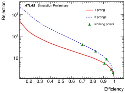
criteria. In addition, an upper cut of 20 GeV is applied on the amount of missing transverse energy in the event in order to suppress contamination from W → l ν +jets events. The performance of the BDT algorithm has been evaluated on an independent set of simulated Z → ττ events for signal efficiency and simulated QCD dijet events for background rejection. The performance has been evaluated for true τ had-vis candidates and also for τ had-vis satisfying the offline tau identification criteria in order to ensure maximal overlap between online and offline identification criteria. Working points of the BDT are tuned separately for 1-prong and multi-prong candidates. Figure 1 shows the performance of the BDT algorithm for τ had-vis candidates reconstructed offline as 1-prong and 3-prong and passing the HLT p T and track multiplicity requirements. The baseline medium working point yields an efficiency of 96 % (82 %) for true 1-prong (3-prong) τ had-vis that are reconstructed offline as 1-prong (3-prong) τ had-vis and pass the HLT p T and track multiplicity requirements.
Efficiency 0.2 0.3 0.4 0.5 0.6 0.7 0.8 0.9 1
Rejection
10 10
210
31 prong 3 prongs working points ATLAS Simulation Preliminary
Figure 1: Performance of the BDT algorithm in terms of background rejection as a function of the signal efficiency for 1-prong and 3-prong τ had-vis candidates reconstructed offline as 1-prong and 3-prong τ had-vis and passing the HLT p T and track multiplicity requirements. The working points correspond to the tight , medium and loose identification criteria in order of decreasing background rejection. The efficiency is estimated using simulated Z → ττ events and the rejection is estimated using simulated di-jet QCD events.
3.2.4 Algorithm timing
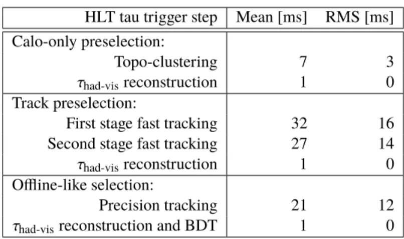
Table 2 summarises the time each step of the HLT tau trigger requires as measured in the data collected on October 26, 2016 at the beginning of the fill when the instantaneous luminosity was about 1 . 2 × 10 34 cm − 2 s − 1 and the pile-up was 40. The majority of the time is spent in executing the fast and precision tracking algorithms. The precision tracking takes less time since it is seeded by the tracks found by the fast tracking.
The full sequence requires about 90 ms to run on the ATLAS TDAQ farm, but this occurs only for the
Table 2: Summary of the execution times of all the steps of the HLT tau trigger as measured in data collected on October 26th 2016 at an instantaneous luminosity of about 1 . 2 × 10 34 cm − 2 s − 1 and pile-up of 40.
HLT tau trigger step Mean [ms] RMS [ms]
Calo-only preselection:
Topo-clustering 7 3
τ had-vis reconstruction 1 0
Track preselection:
First stage fast tracking 32 16
Second stage fast tracking 27 14
τ had-vis reconstruction 1 0
Offline-like selection:
Precision tracking 21 12
τ had-vis reconstruction and BDT 1 0
τ had-vis candidates surviving the intermediate selections based on p T and track multiplicities. Moreover, for each event all computed information is cached so that other tau triggers do not need to compute it again.
4 Trigger menu and rates
The primary tau triggers consist of triggers for single high- p T τ had-vis , and combined τ + X triggers, where X stands for an electron, muon, a second τ had-vis or E miss
T . Table 3 lists the selections used in these triggers in 2016, together with the typical corresponding offline selections and their rates at L1 and the HLT in pp collisions at
√ s = 13 TeV at the instantaneous luminosity of 1 . 2 × 10 34 cm − 2 s − 1 . Besides the p T thresholds, the baseline tau trigger selection includes the L1 isolation requirement, the cuts on the track multiplicities and the medium identification criterion, as described in Section 3, if not otherwise indicated. Due to L1 rate limitations, the combined triggers τ + e/µ/τ and τ + E miss
T require the presence of an additional jet candidate at L1 with transverse momentum above 25 and 20 GeV, respectively. No jet requirement is applied at the HLT because no additional rate reduction is needed.
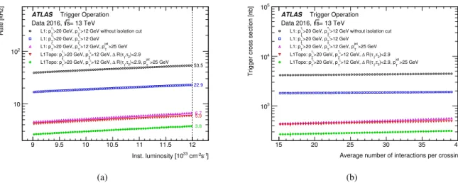
Figure 2(a) shows the L1 rates for these primary tau triggers as a function of the instantaneous luminosity,
while Figure 2(b) shows the trigger cross section as a function of the average number of interactions per
bunch-crossing. The trigger cross section is computed as the trigger rate divided by the instantaneous
luminosity and it is used to check the dependence of the trigger rate on the pile-up. Figure 2(b) shows that
the single tau trigger has no dependence on the average number of interactions per bunch-crossing given
the high p T threshold, in contrast to the combined triggers that show a moderate dependence.
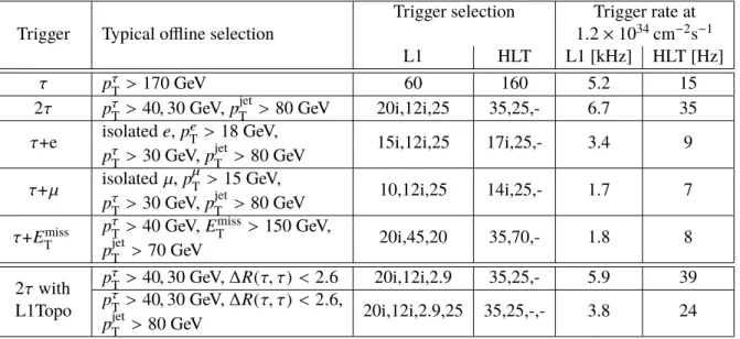
Table 3: Primary tau triggers used in the 2016 pp data taking period. For each trigger, the typical offline selection is indicated, together with the online selections at L1 and the HLT. The online thresholds are matching in the same order to the offline thresholds. When an online selection is not applicable, ‘-’ is indicated. ‘i’ indicates that an isolation requirement is applied at trigger level. The trigger rates are reported for an instantaneous luminosity of 1 . 2 × 10 34 cm − 2 s − 1 and are not unique, that is they do not account for overlaps with other triggers. The L1Topo 2 τ triggers are those commissioned in 2016.
Trigger Typical offline selection
Trigger selection Trigger rate at 1 . 2 × 10 34 cm − 2 s − 1
L1 HLT L1 [kHz] HLT [Hz]
τ p τ
T > 170 GeV 60 160 5.2 15
2 τ p τ
T > 40 , 30 GeV, p jet
T > 80 GeV 20i,12i,25 35,25,- 6.7 35
τ +e isolated e , p e
T > 18 GeV,
15i,12i,25 17i,25,- 3.4 9
p τ
T > 30 GeV, p jet
T > 80 GeV τ + µ isolated µ , p µ
T > 15 GeV,
10,12i,25 14i,25,- 1.7 7
p τ
T > 30 GeV, p jet
T > 80 GeV τ + E miss
T
p τ
T > 40 GeV, E miss
T > 150 GeV,
20i,45,20 35,70,- 1.8 8
p jet
T > 70 GeV 2 τ with
L1Topo p τ
T > 40 , 30 GeV, ∆R(τ, τ) < 2 . 6 20i,12i,2.9 35,25,- 5.9 39 p τ
T > 40 , 30 GeV, ∆R(τ, τ) < 2 . 6,
20i,12i,2.9,25 35,25,-,- 3.8 24 p jet
T > 80 GeV
-1]
-2s
33 cm Inst. luminosity [10
9 9.5 10 10.5 11 11.5 12
Rate [kHz]
1 10
6.7
5.2
3.4
1.8 1.7
= 13 TeV s Data 2016,
ATLAS Trigger Operation
>25 GeV T
>12 GeV, pjet T τ2
>20 GeV, p T τ1
L1: p
>60 GeV T L1: pτ
>25 GeV T
>12 GeV, pjet T
>15 GeV, pτ T L1: pe
>20 GeV T
>45 GeV, pjet T
>20 GeV, Emiss T L1: pτ
>25 GeV T
>12 GeV, pjet T
>10 GeV, pτ T L1: pµ
(a)
Average number of interactions per crossing
15 20 25 30 35 40
Trigger cross section [nb]
0 100 200 300 400 500 600 700 800 900 1000
= 13 TeV s Data 2016,
ATLAS Trigger Operation
>25 GeV T
>12 GeV, pjet T τ2
>20 GeV, p T τ1
L1: p
>60 GeV T L1: pτ
>25 GeV T
>12 GeV, pjet T
>15 GeV, pτ T L1: pe
>20 GeV T
>45 GeV, pjet T
>20 GeV, Emiss T L1: pτ
>25 GeV T
>12 GeV, pjet T
>10 GeV, pτ T L1: pµ
(b) Figure 2: L1 rates for the primary τ ( + X ) triggers in pp collisions recorded at
√ s = 13 TeV in 2016. (a) L1 rates
as a function of the instantaneous luminosity. Rates are shown between 0.9 and 1 . 2 × 10 34 cm − 2 s − 1 . Rates at
1 . 2 × 10 34 cm − 2 s − 1 are also indicated in numbers. (b) L1 trigger cross sections as a function of number of interactions
per bunch-crossing.
-1]
-2s
33 cm Inst. luminosity [10
9 9.5 10 10.5 11 11.5 12
Rate [kHz]
10 102
53.5
22.9
6.7 5.9 3.8
= 13 TeV s Data 2016,
ATLAS Trigger Operation
>12 GeV without isolation cut T
2 τ
>20 GeV, p T τ1
L1: p
>12 GeV T
2 τ
>20 GeV, p T
1 τ L1: p
>25 GeV T jet
>12 GeV, p T
2 τ
>20 GeV, p T
1 τ L1: p
)<2.9 τ2 1, R(τ
>12 GeV, ∆ T
2 τ
>20 GeV, p T τ1
L1Topo: p
>25 GeV T )<2.9, pjet τ2 1, R(τ
>12 GeV, ∆ T
2 τ
>20 GeV, p T
1 τ L1Topo: p
(a)
Average number of interactions per crossing
15 20 25 30 35 40
Trigger cross section [nb]
103
104
105
= 13 TeV s Data 2016,
ATLAS Trigger Operation
>12 GeV without isolation cut T
2 τ
>20 GeV, p T τ1
L1: p
>12 GeV T
2 τ
>20 GeV, p T
1 τ L1: p
>25 GeV T jet
>12 GeV, p T
2 τ
>20 GeV, p T
1 τ L1: p
)<2.9 τ2 1, R(τ
>12 GeV, ∆ T
2 τ
>20 GeV, p T τ1
L1Topo: p
>25 GeV T )<2.9, pjet τ2 1, R(τ
>12 GeV, ∆ T
2 τ
>20 GeV, p T
1 τ L1Topo: p
(b)
Figure 3: Comparison of the L1 rates for several 2 τ triggers, including those using L1Topo, in pp collisions recorded at
√ s = 13 TeV in 2016. The isolation requirement is always applied on both τ had-vis candidates, except when
otherwise mentioned. (a) L1 rates as a function of the instantaneous luminosity. Rates are shown between 0.9 and 1 . 2 × 10 34 cm − 2 s − 1 . Rates at 1 . 2 × 10 34 cm − 2 s − 1 are also indicated in numbers. (b) L1 trigger cross sections as a function of number of interactions per bunch-crossing.
4.1 2τ triggers and L1Topo commissioning
Among the tau triggers, the 2 τ trigger is of highest priority due to its importance for the measurement of the coupling of the Higgs boson to fermions. To ensure high signal acceptance, it is essential that both τ had-vis p T thresholds are set as low as possible and this calls for alternative strategies to reduce the L1 trigger rate.
The L1 rate reduction of the 2 τ trigger has been particularly critical in 2016, when the peak instantaneous luminosity exceeded the LHC design value of 10 34 cm − 2 s − 1 by almost 40%. Even higher luminosities are expected in 2017.
Since at L1 only calorimeter information is available, the ability to reduce the L1 rate without increasing the τ had-vis p T threshold is only by means of isolation requirements on each τ had-vis candidate and event-wise topological requirements. Figures 3(a) and 3(b) show the impacts of such selections on the L1 trigger rates and trigger cross sections of the 2 τ trigger, respectively.
At 1 . 2 × 10 34 cm − 2 s − 1 , for a 2 τ trigger with L1 τ had-vis p T thresholds of 20 and 12 GeV, the L1 isolation
(Section 3.1) reduces the rate from 54 to 23 kHz. To further reduce the rate, the primary 2 τ trigger used
throughout 2016 requires the presence of an additional jet with p T > 25 GeV. This requirement is motivated
by the fact that the target H → 2 τ had-vis + 2 ν analysis is performed only in events with boosted τ had-vis
pairs [2]. Typically, a ∆R offline (τ, τ ) < 2 . 4 requirement is applied in the signal regions. Since geometric
selections cannot be implemented in L1Calo, the L1 jet requirement is used to trigger on the jet activity
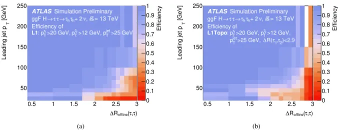
recoiling from the boosted τ had-vis pair. Such selection brings the rate down to 6.7 kHz and its efficiency
in simulated Higgs boson events is shown in Figure 4(a) as a function of the ∆R offline (τ, τ) between the
two offline reconstructed τ had-vis candidates and the transverse momentum of the leading jet reconstructed
offline. The strong correlation between the efficiency as a function of ∆R offline (τ, τ) and the efficiency as
) , τ R
offline( τ
∆
0.5 1 1.5 2 2.5 3
[GeV]
TLeading jet p
50 100 150 200 250
Efficiency
0 0.1 0.2 0.3 0.4 0.5 0.6 0.7 0.8 0.9 Simulation Preliminary 1
ATLAS
= 13 TeV , s Efficiency of
>25 GeV
jet
>12 GeV, p
T T2>20 GeV, p
τ T1: p
τL1
+ 2 ν τ
hτ
h→ τ τ ggF H →
(a)
) , τ R
offline( τ
∆
0.5 1 1.5 2 2.5 3
[GeV]
TLeading jet p
50 100 150 200 250
Efficiency
0 0.1 0.2 0.3 0.4 0.5 0.6 0.7 0.8 0.9 Simulation Preliminary 1
ATLAS
= 13 TeV , s Efficiency of
)<2.9 τ
2 1, R( τ
>25 GeV, ∆
jet
p
T>12 GeV,
T2
>20 GeV, p
τ T1: p
τL1Topo
+ 2 ν τ
hτ
h→ τ τ ggF H →
(b)
Figure 4: Efficiencies for the topological requirements at L1 in the 2 τ trigger in H → 2 τ had-vis + 2 ν events produced via gluon fusion and simulated at
√ s = 13 TeV: (a) requirement of an additional jet with p T > 25 GeV implemented at L1Calo; (b) requirement at L1Topo of an additional jet with p T > 25 GeV and non overlapping with the two L1 τ had-vis candidates, and ∆R(τ, τ) < 2 . 9 implemented. The efficiency is computed with respect to the events passing the 2 τ trigger without the topological requirement. It is plotted as a function of the ∆R offline (τ, τ) between the two offline reconstructed τ had-vis candidates and the transverse momentum of the leading jet reconstructed offline. No offline selection is applied besides the presence of two τ had-vis candidates and at least one jet with p T > 20 GeV.
a function of the leading jet p T is expected from the kinematic correlation of these two variables in signal events.
More effective selections are allowed by the L1Topo hardware. The algorithms implemented in the 2 τ trigger take the lists of isolated L1 τ had-vis objects and L1 jets reconstructed by L1Calo and compute the
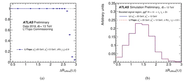
∆R between these objects to find either pairs of τ had-vis with small ∆R or pairs of non-overlapping τ had-vis and jet. The requirement of ∆R(τ, τ) < 2 . 9 is effective in reducing the L1 rate. Indeed, at L1 the angular resolution is better than the p T resolution and this leads to sharper turn-on curves in the efficiency and a more effective rate reduction. Figure 5 shows the performance in acceptance of the ∆R(τ, τ) < 2 . 9 selection implemented in L1Topo for data and simulation. This selection is fully efficient for offline τ had-vis pairs with ∆R offline (τ, τ ) . 2 . 6 (Figure 5(a)) and leads to no loss in signal acceptance in the signal regions used for the H → ττ search. Figure 5(b) shows the ∆R offline (τ, τ) distribution of the signal events accepted in the “Boosted” signal region used in Ref. [2], where the p T of the reconstructed Higgs boson candidate is required to be above 100 GeV. To illustrate the impact of the ∆R(τ, τ) selection at L1Topo, no selection on
∆R offline (τ, τ ) is applied. Without any H → ττ event loss, this selection allows for a rate reduction of the 2 τ trigger from 23 to 5.9 kHz at 1 . 2 × 10 34 cm − 2 s − 1 (Table 3), a rate even lower than the one reached with the jet requirement implemented at L1Calo (6.7 kHz). As shown in Figure 3(b), the L1Topo ∆R(τ, τ) selection has also a reduced dependence on pile-up compared to the L1 trigger with jet requirement. Although the same HLT criteria for the two τ had-vis candidates are applied in the configuration with L1Topo and in the one without L1Topo, the HLT rate reduction is not as strong: the rate for the 2 τ trigger with the L1Topo
∆R(τ, τ ) selection is 39 Hz, while the rate for the 2 τ trigger with the additional jet at L1Calo is 35 Hz.
Given that the HLT selection is the same, this effect suggests that the two L1 selections are not accepting the
) , τ R
offline( τ
∆
0.5 1 1.5 2 2.5 3
Efficiency
0 0.2 0.4 0.6 0.8 1
ATLAS Preliminary
= 13 TeV s Data 2016,L1Topo Commissioning
)<2.9 τ2 1, R(τ
>12 GeV, ∆
T 2 τ
>20 GeV, p
T 1
: pτ
L1Topo
(a)
) , τ R
offline( τ
∆
0.5 1 1.5 2 2.5 3
Arbitrary units
0 0.05 0.1 0.15 0.2 0.25 0.3 0.35
= 13 TeV s
> 12 GeV
T 2 τ
> 20 GeV, p
T τ1
: p L1
) < 2.9 τ2 1, R(τ > 12 GeV, ∆
T 2 τ
> 20 GeV, p
T 1
: pτ
L1Topo
Simulation Preliminary, ATLAS
+ 2ν τh
τh
→ τ τ Boosted signal region, ggF H →
(b)
Figure 5: Performance of the ∆R(τ, τ) < 2 . 9 selection implemented at L1Topo in the 2 τ trigger in data and in simulation. The acceptance is shown with respect to the events passing the 2 τ trigger without the L1Topo ∆R(τ, τ) requirement and is plotted as a function of the ∆R offline (τ, τ) between the two offline reconstructed τ had-vis candidates.
(a) Efficiency of the L1Topo ∆R(τ, τ) selection in data. (b) Comparison of event acceptances of the 2 τ triggers with and without the L1Topo ∆R(τ, τ) selection in H → 2 τ had-vis + 2 ν events produced via gluon fusion and simulated at
√ s = 13 TeV. The “Boosted” selection [2] without any selection on ∆R offline (τ, τ) is applied.
same background events and, indeed, when these two selections are applied together an even stronger L1 rate reduction down to 3.8 kHz is achieved. The L1Topo algorithm implementing this combined selection requires a pair of τ had-vis candidates with ∆R( τ, τ) < 2 . 9 and a jet candidate with p T > 25 GeV and with
∆R(τ, j) > 0 . 1 with respect to each of the τ had-vis candidates in the selected pair. The efficiency of this L1Topo selection in H → ττ events is shown in Figure 4(b).
5 Performance and efficiency
This section describes the ‘tag-and-probe’ analyses used to measure the efficiency of the tau trigger and to validate the online τ had-vis reconstruction and identification. These analyses target Z → µτ had-vis 3 ν events, where one tau lepton decays leptonically into a muon and the second tau lepton decays hadronically, and t¯ t → [ bµν ][ bτ had-vis 2 ν ] events, where both top quarks decay leptonically into a muon and a hadronically decaying tau lepton. The Z → µτ had-vis 3 ν analysis profits from high statistics and good purity, while the t¯ t → [ b µν ][ bτ had-vis 2 ν ] analysis yields τ had-vis candidates up to higher transverse momenta.
The pp collision data used for these measurements were recorded in 2016 at a centre-of-mass energy of
√
s = 13 TeV, and correspond to an integrated luminosity of 33 fb − 1 . Signal and background samples are
produced using Monte Carlo generators, as detailed in Table 4, and reconstructed with the same algorithms
as the data. The simulation accounts for the effect of multiple proton-proton interactions per bunch-crossing
in data. Data-driven corrections to the reconstruction and selection of the muon and τ had-vis candidates
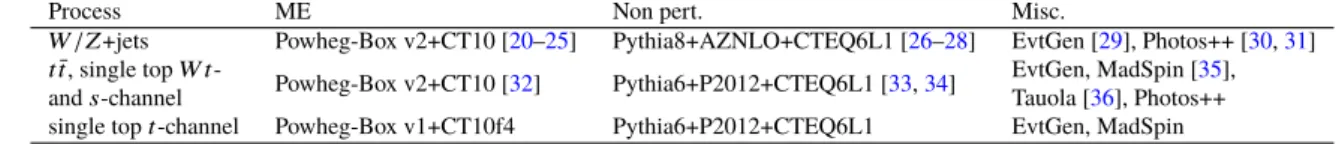
Table 4: Details of the software used in simulation, including: the generation of the matrix element and the corresponding PDF set (ME); and the modelling of non-perturbative effects (Non pert.) such as the parton shower, MC tune and PDF set (if different than for ME). The following additional software (Misc.) is used in some cases:
EvtGen to set the properties of the bottom and charm hadron decays, Photos++ for QED emissions from electroweak vertices and charged leptons, Tauola for the decay of tau leptons and MadSpin for the decay of top quarks.
Process ME Non pert. Misc.
W /Z +jets Powheg-Box v2+CT10 [20–25] Pythia8+AZNLO+CTEQ6L1 [26–28] EvtGen [29], Photos++ [30, 31]
t t ¯ , single top W t -
Powheg-Box v2+CT10 [32] Pythia6+P2012+CTEQ6L1 [33, 34] EvtGen, MadSpin [35],
and s -channel Tauola [36], Photos++
single top t -channel Powheg-Box v1+CT10f4 Pythia6+P2012+CTEQ6L1 EvtGen, MadSpin
are applied to ensure agreement between data and simulation. Similar measurements performed on data collected in 2015 are documented in Ref. [19].
5.1 Tag-and-probe preselection
Events are selected by requiring the presence of a muon, the tag , selected by the lowest unprescaled single- muon trigger available in each data period, and an offline reconstructed τ had − vis candidate, the probe . This selection is summarised in Table 5.
The tag muon is reconstructed by combining an inner-detector track with a track from the muon spectro- meter [37]. It is required to have |η | < 2 . 5 and to pass calorimeter and track isolation requirements. The muon transverse momentum must be at least 2 GeV higher than that required by the muon trigger; that is, 26 GeV in the first 6.1 fb − 1 and 28 GeV in the remaining 27.1 fb − 1 of the 2016 pp data. Events with more than one muon are vetoed. Corrections to the muon trigger and reconstruction efficiencies derived from the data are applied to the simulated samples.
The reconstruction and identification of τ had-vis candidates is described in detail in Refs. [15, 18]. In this note, the τ had-vis probe is required to have p T > 25 GeV, |η| < 2 . 5 (excluding the region 1 . 37 < |η| < 1 . 52), one or three core tracks and electric charge opposite to the charge of the muon. The τ had-vis probe is also required to satisfy the medium identification criterion of the BDT discriminant against jets.
Events with electrons reconstructed with p T > 15 GeV in |η | < 2 . 5 (excluding 1 . 37 < |η | < 1 . 52) and passing the loose likelihood identification are vetoed [38]. Geometric overlap of objects with ∆R < 0 . 2 is resolved by selecting only one of the overlapping objects in the following order of priority: muons, electrons, τ had-vis and jets. The missing transverse energy E miss
T is calculated from the vector sum of the transverse momenta of all reconstructed electrons, muons, τ had-vis and jets in the event, as well as a term for the remaining soft activity in the calorimeter [39].
5.2 Z → µτ had-vis 3ν selection and background estimation
As indicated in Table 5, the purity of Z → µτ had-vis 3 ν events is enhanced with further requirements on
the selected tag-probe pair. The muon tag and the τ had-vis probe are required to have an invariant mass
m vis (τ had-vis , µ) between 45 and 80 GeV. To reduce the background contamination from W (→ µν) + jets
Table 5: Summary of the Z → µτ had-vis 3 ν and t t ¯ → [ b µν ][ bτ had-vis 2 ν ] tag-and-probe event selections.
Event preselection
Muon tag: τ had-vis probe:
Medium quality jet BDT medium
Trigger-matched Muon veto, no overlapping electron p T > 26 / 28 GeV p T > 25 GeV , |q | = 1
|η | < 2 . 5 |η | < 1 . 37, 1 . 52 < |η | < 2 . 47 track+calo isolation 1 or 3 core tracks
Tag-probe pair selection:
muon and τ had-vis with opposite electric charge No other muon or electron
Z → µτ had-vis 3 ν t¯ t → [ bµν ][ bτ had-vis 2 ν ] m T ( µ, E miss
T ) < 50 GeV At least 2 jets
Σ cos ∆φ > − 0 . 5 At least 1 b -tagged jet 45 GeV < m vis (τ had-vis , µ) < 80 GeV
events, the transverse mass m T ( µ, E miss
T ) = q
2 p µ
T E miss
T
1 − cos ∆φ µ, E miss
T must be less than 50 GeV, and the sum of the azimuthal angles of the muon and the τ had-vis with the missing energy Σ cos ∆φ = cos ∆ φ(τ had-vis , E miss
T ) + cos ∆ φ( µ, E miss
T ) must be greater than -0.5.
The main backgrounds to this measurement are multi-jet and W (→ µν) + jets where a jet is misidentified as τ had-vis ( j → τ ). In a small fraction of events the selected probe is a lepton ( l → τ ). A combination of data-driven and simulation-based approaches is used to model these backgrounds, similar to those used in Ref. [15]. The full estimate of the background in the opposite-sign (OS) signal region (SR) is written as
N fake
OS = R OS / SS · Data SS + W µν OS − SS + Z µµ OS − SS + top OS − SS , (1) where each term is detailed in the following. The “OS − SS” superscript indicates the subtraction that is used to determine the charge asymmetric contribution to be added to the data with same-sign (SS) tag-probe pairs.
The R OS / SS · Data SS term accounts for the multi-jet background and the charge-symmetric components
of the other background processes, like W (→ µν) + jets, top and Z (→ µµ) + jets. It is modelled using
Data SS ; data in the SS control region where the charge-product between the tag and the probe is positive,
and a negligible Z → µτ had-vis 3 ν contamination is found. As the expected number of background events
depends on the charge-product between the tag and the probe, the normalisation of the SS data is corrected
by the R OS / SS factor. This factor is measured in a multi-jet enriched control region defined by inverting
the isolation requirement around the tag muon. The R OS / SS factor is the ratio of the number of events
in OS and SS data, and is parametrised using the probe τ had-vis track multiplicity and the muon p T , and
is independently measured before and after the tau trigger. Uncertainties on the R OS / SS scale factor are
calculated by varying the muon isolation selection which define the R OS / SS control region. The values for the R OS / SS factor range between 1.16 and 1.55 and their uncertainties are approximately 5%.
The W µν OS − SS term accounts for the charge-asymmetric component of the W (→ µν) + jets background, which is added to the charge-symmetric component included in the R OS / SS Data SS term. This contribution is modelled using data from the low- Σ cos ∆φ region, defined by removing the m T ( µ, E miss
T ) selection and inverting the Σ cos ∆φ requirement indicated in Table 5. In such a region, the OS data are used after subtracting the SS data scaled by R OS / SS and removing the expected small contributions from Z → µµ , Z → µτ had-vis 3 ν , and top events based on simulation. The normalisation of this data is corrected by the ratio of the W (→ µν) + jets yield in the signal region to the yield in the low- Σ cos ∆φ region, as expected in simulation.
The remaining Z µµ OS − SS and top OS − SS terms are the charge-asymmetric contributions from Z (→ µµ) +jets and events with top quarks to be added to the charge-symmetric components included in R OS / SS · Data SS . They are estimated as:
N OS − SS = kW OS N OS j→τ − kW SS R OS / SS · N SS j→τ + N OS l→τ − R OS / SS · N SS l→τ , (2) where “N” is either the Z → µµ or the top contribution based on simulation; kW OS ( SS ) is a data-driven correction to the normalisation of the j → τ OS(SS) events; N j→τ OS(SS) is expected j → τ contribution in OS(SS) events; and N l→τ OS ( SS ) is expected l → τ contribution in OS(SS) events. The kW corrections account for possible mismodellings of the j → τ fake rate in simulation, and are measured in a control region enriched in W (→ µν) + jets events, defined by m T ( µ, E miss
T ) > 60 GeV and E miss
T > 30 GeV with respect to the selection applied in the signal region (Table 5). This correction is the ratio between the observed data and the W (→ µν) + jets events expected from simulation. Uncertainties on the kW factors are measured by varying the cut on m T ( µ, E miss
T ) , which defines the W (→ µν) + jets control region. The values for the kW factors range between 1.35 and 1.94 and their uncertainties are approximately 2%. For the simulated charge-asymmetric component of the l → τ background no data-driven correction is applied as this contribution is found to be negligible.
The contribution from top events with true τ had-vis as expected from simulation is excluded from the top OS − SS term and is subtracted from data in all the control regions. The contribution of Z → µτ had-vis 3 ν events where the probe is a misidentified jet is found to be negligible.
The systematic uncertainties relevant for trigger efficiency measurement are those on the background estimation. They include the uncertainties on the trigger, reconstruction and selection efficiency of the tag muon, on the luminosity and the R OS / SS and kW factors. Further systematic uncertainties are included for the soft term of the E miss
T , and pile-up reweighting. Systematic uncertainties on the τ had-vis probe reconstruction and identification efficiencies are also estimated, but they do not impact the efficiency measurement. The overall systematic uncertainty is measured by comparing the yields of background events with and without each systematic variation.
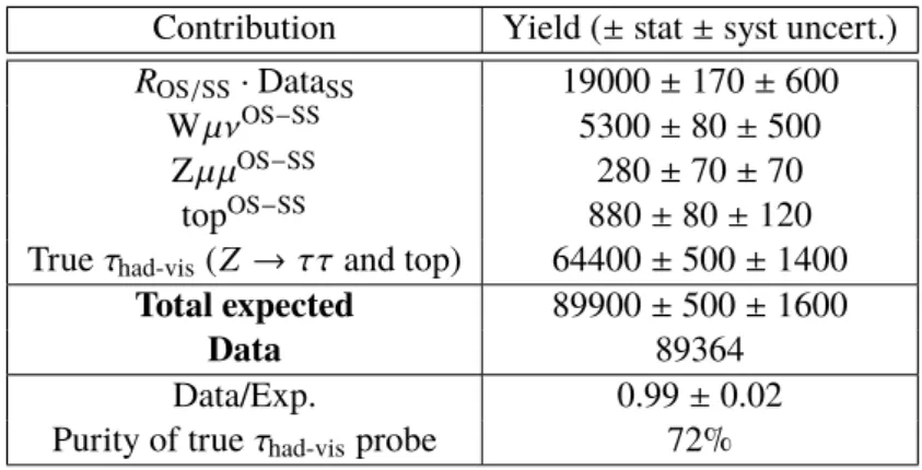
Table 6 reports the observed data and expected signal and background contributions in the OS signal region.
The selected sample of events has an estimated purity of 72% for true τ had-vis probes.
Table 6: Observed and expected event yields after the Z → µτ had-vis 3 ν tag-and-probe event selection in the 33 fb − 1 of 2016 pp collision data. Statistical and systematic uncertainties are reported.
Contribution Yield ( ± stat ± syst uncert.) R OS / SS · Data SS 19000 ± 170 ± 600
W µν OS − SS 5300 ± 80 ± 500
Z µµ OS − SS 280 ± 70 ± 70
top OS − SS 880 ± 80 ± 120
True τ had-vis ( Z → ττ and top) 64400 ± 500 ± 1400 Total expected 89900 ± 500 ± 1600
Data 89364
Data/Exp. 0.99 ± 0.02
Purity of true τ had-vis probe 72%
Figure 6 shows the transverse momentum, the pseudorapidity, the core track multiplicity and the BDT jet score of the selected offline τ had-vis probes. A good agreement between observed data and estimated signal and background contributions is achieved.
5.3 t ¯ t → [bµν ][bτ had-vis 2ν ] selection and background estimation
For the t¯ t → [ bµν ][ bτ had-vis 2 ν ] measurement, further selections on jets are applied on the preselected events. Jets [40] are selected if they are reconstructed with p T > 20 GeV and |η | < 4 . 5. For jets with p T < 50 GeV and |η| < 2 . 4, a requirement on the Jet Vertex Tagger (JVT) [41] to be greater than 0.64 is used to increase the rejection of pile-up jets. Jets coming from a b -quark ( b -tagged) are identified using a multivariate b -tagging algorithm with a target efficiency of 85% [42]. As indicated in Table 5, in order to suppress non- t t ¯ processes and obtain a high purity, only events with at least two jets, one of which is b -tagged, are used.
As for the Z → µτ had-vis 3 ν analysis, most of the background events have a jet misidentified as a probe
τ had-vis . The sources for such events are t t ¯ , single top quark, electroweak and multi-jet events. In a
small fraction of background events, the probe τ had-vis is a misidentified lepton. The estimation of these
background events is based on the same method as described in Section 5.2 and Equation 1, with few
differences. The R OS / SS · Data SS term is based on the same method and is determined using the data
selected by modifying the selections on the tag-probe charge product and on the muon isolation with
respect to the t¯ t → [ bµν ][ bτ had-vis 2 ν ] selection in Table 5. The values for the R OS / SS factor determined
in this analysis range between 1.05 and 1.23 and their uncertainties are between 2% and 13%. Given
the negligible contribution of W ( → µν) + jets events, the W µν OS − SS term is estimated from simulation
as the other charge-asymmetric contributions from top events. The misidentification rate and the trigger
efficiencies in these j → τ simulated contributions are corrected by the same kW OS and kW SS factors
estimated in the Z → µτ had-vis 3 ν measurement.
20 30 40 50 60 70 80 90 100
Events / 4.0 GeV
5000 10000 15000 20000 25000 30000 35000 40000
Data True τ
Same Sign W →µν (OS-SS) (OS-SS)
µ µ
Z → Top (OS-SS)
Sys. + stat. unc.
Preliminary ATLAS 33 fb-1
= 13 TeV s
had µτ τ Z→
[GeV]
Offline tau p
T20 30 40 50 60 70 80 90 100
Data/exp.
0.6 0.8 1 1.2 1.4
(a) Transverse momentum
3
− −2 −1 0 1 2 3
Events / 0.5
2000 4000 6000 8000 10000 12000 14000 16000 18000
20000 Data True τ
Same Sign W →µν (OS-SS) (OS-SS)
µ µ
Z → Top (OS-SS)
Sys. + stat. unc.
Preliminary ATLAS 33 fb-1
= 13 TeV s
had µτ τ Z→
Offline tau η
3− −2 −1 0 1 2 3
Data/exp.
0.6 0.8 1 1.2 1.4
(b) Pseudorapidity
1 2 3 4
Events
20 40 60 80 100
103
×
Data True τ
Same Sign W →µν (OS-SS) (OS-SS)
µ µ
Z → Top (OS-SS)
Sys. + stat. unc.
Preliminary ATLAS 33 fb-1
= 13 TeV s
had µτ τ Z→
tracks
Offline tau N
1 2 3 4
Data/exp.
0.6 0.8 1 1.2 1.4
(c) Core track multiplicity
0.6 0.65 0.7 0.75 0.8 0.85 0.9 0.95 1
Events / 0.02
2000 4000 6000 8000 10000 12000 14000 16000 18000 20000
Data True τ
Same Sign W →µν (OS-SS) (OS-SS)
µ µ
Z → Top (OS-SS)
Sys. + stat. unc.
Preliminary ATLAS 33 fb-1
= 13 TeV s
had τ τµ Z→
Offline tau BDT score
0.6 0.65 0.7 0.75 0.8 0.85 0.9 0.95 1
Data/exp.
0.6 0.8 1 1.2 1.4
(d) Jet BDT score
Figure 6: Kinematics and properties of the offline τ had-vis probes after the Z → µτ had-vis 3 ν tag-and-probe event
selection. Both systematic and statistical uncertainties are shown.
Table 7: Observed and expected event yields after the t t ¯ → [ bµν ][ bτ had-vis 2 ν ] tag-and-probe event selection in the 33 fb − 1 of 2016 pp collision data. Statistical and systematic uncertainties are reported.
Contribution Yield ( ± stat ± syst uncert.) R OS / SS · Data SS 8900 ± 100 ± 400 j → τ (OS-SS) 6100 ± 200 ± 700
l → τ (OS-SS) 1070 ± 50 ± 100
True τ had-vis 25600 ± 120 ± 2600
Total expected 41800 ± 300 ± 2700
Data 44074
Data/Exp. 1.06 ± 0.06
Purity of true τ had-vis probe 61%
In addition to the sources of systematic uncertainties on the background estimate described in Section 5.2, uncertainties on the b -tagging (in)efficiency are also considered. The dominant uncertainty on the back- ground is the first eigenvector of the b-tag systematics of about 2.2%. Other significant uncertainties are on the luminosity (2.0%) and the kW factors (1.7%).
Table 7 reports the observed data and expected signal and background contributions in the OS signal region.
The selected sample of events has an estimated purity of 61% for true τ had-vis probes. Figure 7 shows the transverse momentum, the pseudorapidity, the core track multiplicity and the BDT jet score of the selected offline τ had-vis probes.
5.4 Online tau reconstruction performance
The modelling and the performance of the τ had-vis reconstruction in the tau trigger is validated by comparing the properties of the online τ had-vis candidate between simulation and data. Out of the events selected in the Z → µτ had-vis 3 ν analysis (Section 5.2), only those where the offline τ had-vis probe is matched within
∆R < 0 . 2 to an online τ had-vis candidate are used in this comparison. The online selection requires at L1
an isolated candidate with E T > 12 GeV, and p T > 25 GeV at the HLT. No HLT identification or track
multiplicity requirements are applied. However, this sample of online τ had-vis candidates is biased by the
identification and track multiplicity selections applied on the matching offline probe. Here and in all the
following plots, the background contributions as determined in Section 5.2 are plotted together as fakes .
Figure 8 shows transverse momentum, pseudorapidity, azimuthal angle and core track multiplicity of the
online τ had-vis candidates as reconstructed at the final stage of the HLT tau trigger. Figures 9 to 12 show the
input variables used for the HLT BDT identification listed in Table 1. A good modelling is observed in all
these distributions.
Events / 10 GeV
0 2000 4000 6000 8000 10000 12000 14000 16000 18000 20000
Data 2016
had-vis
True τ (OS-SS) τ l →
(OS-SS) τ j →
DataSS OS/SS
R
Syst. Unc.
Stat. ⊕
ATLAS Preliminary
= 13 TeV, 33 fb
-1s t t
[GeV]
Offline tau p
T0 20 40 60 80 100 120 140 160 180 200
Data / Background
0.6 0.8 1 1.2 1.4
(a) Transverse momentum
Events
0 1000 2000 3000 4000 5000 6000 7000
Data 2016
had-vis
τ True
(OS-SS) τ
→ l
(OS-SS) τ
→ j
DataSS OS/SS
R
Syst. Unc.
⊕ Stat.
ATLAS Preliminary = 13 TeV, 33 fb
-1s t t
Offline tau η
−3 −2 −1 0 1 2 3
Data / Background
0.6 0.8 1 1.2 1.4
(b) Pseudorapidity
Events
0 10000 20000 30000 40000 50000
Data 2016
had-vis
True τ (OS-SS) τ l →
(OS-SS) τ j →
DataSS OS/SS
R
Syst. Unc.
Stat. ⊕
ATLAS Preliminary
= 13 TeV, 33 fb
-1s t t
track
Offline tau N
0 1 2 3 4 5 6
Data / Background
0.6 0.8 1 1.2 1.4
(c) Core track multiplicity
Events
0 2000 4000 6000 8000 10000 12000 14000 16000 18000 20000
Data 2016
had-vis
True τ (OS-SS) τ l →
(OS-SS) τ j →
DataSS OS/SS
R
Syst. Unc.
Stat. ⊕
ATLAS Preliminary
= 13 TeV, 33 fb
-1s t t
Offline tau BDT score
0.5 0.6 0.7 0.8 0.9 1 1.1 1.2
Data / Background
0.6 0.8 1 1.2 1.4
(d) Jet BDT score
Figure 7: Kinematics and properties of the offline τ had-vis probes after the t t ¯ → [ b µν ][ bτ had-vis 2 ν ] tag-and-probe event
selection. Both systematic and statistical uncertainties are shown.
20 30 40 50 60 70 80 90 100
Events / 4.0 GeV
5000 10000 15000 20000 25000
Data True τ Fakes Sys. + stat. unc.
Preliminary ATLAS
= 13 TeV s
-1, 33 fb
had
µτ τ Z→ 1-prong
[GeV]
HLT tau pT
20 30 40 50 60 70 80 90 100
Data/exp.
0.6 0.8 1 1.2 1.4
(a) HLT τ had-vis p T
20 30 40 50 60 70 80 90 100
Events / 4.0 GeV
1000 2000 3000 4000 5000
6000 Data
True τ Fakes Sys. + stat. unc.
Preliminary ATLAS
= 13 TeV s
-1, 33 fb
had
µτ τ Z→ 3-prong
[GeV]
HLT tau pT
20 30 40 50 60 70 80 90 100
Data/exp.
0.6 0.8 1 1.2 1.4
(b) HLT τ had-vis p T
2
− −1 0 1 2
Events / 0.5
2000 4000 6000 8000 10000
12000 Data
True τ Fakes Sys. + stat. unc.
Preliminary ATLAS
= 13 TeV s
-1, 33 fb
had
µτ τ Z→ 1-prong
HLT tau η 2
− −1 0 1 2
Data/exp.
0.6 0.8 1 1.2 1.4
(c) HLT τ had-vis η
2
− −1 0 1 2
Events / 0.5
500 1000 1500 2000 2500 3000 3500
Data True τ Fakes Sys. + stat. unc.
Preliminary ATLAS
= 13 TeV s
-1, 33 fb
had
µτ τ Z→ 3-prong
HLT tau η 2
− −1 0 1 2
Data/exp.
0.6 0.8 1 1.2 1.4
(d) HLT τ had-vis η
0 1 2 3 4
Events
10000 20000 30000 40000 50000 60000 70000 80000
90000 Data
True τ Fakes Sys. + stat. unc.
Preliminary ATLAS
= 13 TeV s
-1, 33 fb
had
µτ τ Z→ 1-prong
tracks
HLT tau N
0 1 2 3 4
Data/exp.
0.6 0.8 1 1.2 1.4
(e) HLT τ had-vis N core trk
0 1 2 3 4
Events
2000 4000 6000 8000 10000 12000 14000 16000 18000 20000 22000 24000
Data True τ Fakes Sys. + stat. unc.
Preliminary ATLAS
= 13 TeV s
-1, 33 fb
had
µτ τ Z→ 3-prong
tracks
HLT tau N
0 1 2 3 4
Data/exp.
0.6 0.8 1 1.2 1.4
(f) HLT τ had-vis N core trk
0 0.1 0.2 0.3 0.4 0.5 0.6 0.7 0.8 0.9 1
Events / 0.05
5000 10000 15000 20000 25000 30000
Data True τ Fakes Sys. + stat. unc.
Preliminary ATLAS
= 13 TeV s -1, 33 fb
had τ τµ Z→ 1-prong
HLT tau f
cent0 0.1 0.2 0.3 0.4 0.5 0.6 0.7 0.8 0.9 1
Data/exp.
0.6 0.8 1 1.2 1.4
(a) Central energy fraction
1
− −0.8 −0.6 −0.4 −0.2 0 0.2 0.4 0.6 0.8 1
Events / 0.1
2000 4000 6000 8000 10000 12000 14000
Data True τ Fakes Sys. + stat. unc.
Preliminary ATLAS
= 13 TeV s -1, 33 fb
had τ τµ Z→ 1-prong
track-HAD
HLT tau f
EM 1− −0.8 −0.6 −0.4 −0.2 0 0.2 0.4 0.6 0.8 1
Data/exp.
0.6 0.8 1 1.2 1.4
(b) Fraction of EM energy from charged pions
0 1 2 3 4 5 6 7 8 9 10
Events / 0.5
5000 10000 15000 20000 25000
30000 Data
True τ Fakes Sys. + stat. unc.
Preliminary ATLAS
= 13 TeV s -1, 33 fb
had µτ τ Z→ 1-prong
lead track
HLT tau f
-10 1 2 3 4 5 6 7 8 9 10
Data/exp.
0.6 0.8 1 1.2 1.4
(c) Leading track momentum fraction
0 0.02 0.04 0.06 0.08 0.1 0.12 0.14 0.16 0.18 0.2
Events / 0.01
2000 4000 6000 8000 10000 12000 14000 16000 18000 20000
Data True τ Fakes Sys. + stat. unc.
Preliminary ATLAS
= 13 TeV s -1, 33 fb
had µτ τ Z→ 1-prong
track
HLT tau R
0 0.02 0.04 0.06 0.08 0.1 0.12 0.14 0.16 0.18 0.2Data/exp.
0.6 0.8 1 1.2 1.4
(d) Track radius
Figure 9: HLT BDT inputs for online τ had-vis candidates matched to an offline 1-prong τ had-vis probe in the selected
Z → µτ had-vis 3 ν event candidates.
0 0.5 1 1.5 2 2.5 3
Events / 0.15
5000 10000 15000 20000 25000 30000
Data True τ Fakes Sys. + stat. unc.
Preliminary ATLAS
= 13 TeV s -1, 33 fb
had τ τµ Z→ 1-prong
/P
T EM+trackHLT tau P
T0 0.5 1 1.5 2 2.5 3
Data/exp.
0.6 0.8 1 1.2 1.4
(a) Ratio of track-plus-EM-system to p T
0 1 2 3 4 5 6 7 8 9 10
Events / 0.5
2000 4000 6000 8000 10000 12000 14000 16000
18000 Data
True τ Fakes Sys. + stat. unc.
Preliminary ATLAS
= 13 TeV s -1, 33 fb
had τ τµ Z→ 1-prong
EM track
HLT tau f
0 1 2 3 4 5 6 7 8 9 10
Data/exp.
0.6 0.8 1 1.2 1.4
(b) Ratio of EM energy to track momentum
0 1000 2000 3000 4000 5000 6000
Events / 300.0
5000 10000 15000 20000 25000 30000
Data True τ Fakes Sys. + stat. unc.
Preliminary ATLAS
= 13 TeV s -1, 33 fb
had µτ τ Z→ 1-prong
[MeV]
+ track π0
HLT tau m
0 1000 2000 3000 4000 5000 6000
Data/exp.
0.6 0.8 1 1.2 1.4
(c) Track-plus-EM-system mass
0 0.2 0.4 0.6 0.8 1 1.2 1.4 1.6 1.8 2
Events / 0.1
1000 2000 3000 4000 5000 6000
7000 Data
True τ Fakes Sys. + stat. unc.
Preliminary ATLAS
= 13 TeV s -1, 33 fb
had µτ τ Z→ 1-prong
lead track
HLT tau S
0 0.2 0.4 0.6 0.8 1 1.2 1.4 1.6 1.8 2
Data/exp.
0.6 0.8 1 1.2 1.4
![Table 5: Summary of the Z → µτ had-vis 3 ν and t t ¯ → [ b µν ][ bτ had-vis 2 ν ] tag-and-probe event selections.](https://thumb-eu.123doks.com/thumbv2/1library_info/4004816.1540784/14.892.171.691.204.509/table-summary-µτ-vis-µν-probe-event-selections.webp)