ATLAS-CONF-2012-099 18July2012
ATLAS NOTE
ATLAS-CONF-2012-099
July 18, 2012
Performance of the ATLAS muon trigger in 2011
The ATLAS Collaboration
Abstract
Events with muons in the final state are an important signature for many physics analyses in the harsh environment produced by collisions of high energy protons at high luminosity.
The ATLAS experiment employs a multi-level trigger architecture that selects events in three sequential steps of increasing complexity and accuracy. The Level 1 trigger is implemented with custom built hardware to reduce the event rate from 40 MHz to 75 kHz. The software based higher level triggers refine the trigger decisions reducing the output rate to about 400 Hz. This note presents the performance of the muon trigger evaluated with proton- proton collision data collected in 2011 at a centre-of-mass energy of 7 TeV.
c Copyright 2012 CERN for the benefit of the ATLAS Collaboration.
Reproduction of this article or parts of it is allowed as specified in the CC-BY-3.0 license.
1 Introduction
Muons in the final state are distinctive signatures of many physics studies performed with the collisions of high energy protons, such as searches for the Higgs boson or other new phenomena, as well as the measurements of Standard Model (SM) processes. The precise determination of the muon trigger perfor- mance of the ATLAS detector
1at the LHC is essential for muon-related physics analyses. The ATLAS muon trigger system has been designed to select muons in a wide momentum range with high e
fficiency.
The selection of events with muons by the trigger system is performed in three steps. The signals from fast-response muon trigger detectors are processed by custom built hardware to generate a Level 1 (L1) trigger. The L1 muon system has six programmable p
Tthresholds to label the trigger with p
Tinforma- tion. In addition, the L1 trigger carries the detector position information to be investigated by the next steps. Then the software based High Level Trigger (HLT), which is subdivided into the Level 2 (L2) trigger and Event Filter (EF), reconstructs tracks in the vicinity of the detector region reported by the L1 trigger. The L2 trigger performs a fast reconstruction of muons with a simple algorithm. Then the EF makes use of the offline muon reconstruction software to refine the trigger decision by utilising full detector information.
The ATLAS experiment collected proton-proton collision data in 2011 at a centre-of-mass energy of 7 TeV with maximum instantaneous luminosity of 3.65
×10
33cm
−2s
−1. In order to address a wide variety of physics topics, the ATLAS experiment deployed a set of muon triggers. These are low- p
Tdi- muon triggers for B-physics, a medium-p
Tdi-muon trigger for SM processes and for searches, high- p
Tsingle muon triggers as general purpose triggers and muon triggers in combination with electrons, jets and missing-E
Ttriggers for specific physics processes.
In this note only the high-p
Tsingle muon trigger performance is presented. The performance has been evaluated primarily with the tag-and-probe method using samples containing pairs of muons from the decay of Z bosons [1]. In addition, for the purpose of controlling trigger rates in higher pile-up conditions expected in 2012, the performance of isolated muon triggers has been studied.
2 Muon trigger algorithms
The ATLAS detector is a multipurpose particle physics apparatus with a forward-backward symmetric cylindrical geometry and near 4
πcoverage in solid angle. The detector consists of four major sub- systems, the inner detector (ID), electromagnetic calorimeter (ECal), hadronic calorimeter (HCal) and muon spectrometer (MS). A detailed description of the ATLAS detector can be found elsewhere [2]. The ID measures tracks up to
|η|=2.5 in a solenoidal magnetic field of 2 T with three types of detectors: a silicon pixel detector closest to the interaction point, a silicon strip detector (SCT) surrounding the pixel detector, and a transition radiation straw tube tracker (TRT) covering
|η| <2.0 as the outermost part of the ID. The calorimeter system covers the pseudorapidity range
|η|<4.9 and encloses the ID. The high- granularity liquid-argon electromagnetic sampling calorimeter is divided into one barrel (
|η| <1.475) and two endcap components (1.375
<|η|<3.2). The hadronic calorimeter is placed directly outside the ECal. An iron scintillator-tile calorimeter provides hadronic coverage in the range
|η|<1.7. The endcap and forward regions, spanning 1.5
< |η| <4.9, are instrumented with liquid-argon calorimetry. The calorimeters are then surrounded by the MS. The MS consists of three large air-core superconducting
1ATLAS uses a right-handed coordinate system with thex-axis pointing towards the centre of the LHC ring, and thez-axis along the beam direction. The positivey-axis is defined as pointing upwards. The nominal interaction point is defined as the origin of the coordinate system. The azimuthal angleφis measured around the beam axis, and the polar angleθis the angle from the positivez-axis. The pseudorapidity is defined asη=−log tan(θ/2). The transverse momentumpT, the transverse energy ET are defined in the x−yplane. The distance∆Rin the pseudorapidity-azimuthal angle space is defined as∆R= p∆η2+ ∆φ2.
1
low pT
high pT
5 10 15 m
0 RPC 3 RPC 2
RPC 1
low pT high pT
MDT
MDT
MDT
MD T TGC 1
TGC 2
TGC 3
MD T
MD T TGC EI
TGC FI
XX-LL01V04
Tile Calorimeter
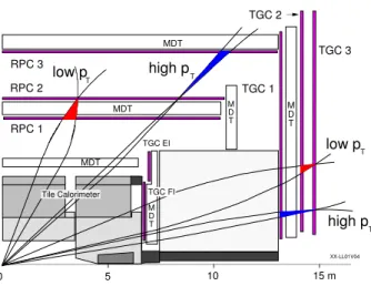
Figure 1: Quarter-section of the muon system in a plane containing the beam axis. The inner most layers of TGCs, TGC EI and TGC FI, are not used for the L1 trigger. CSC detectors are not shown but located at around z
=7 m covering the
ηregion beyond the MDT acceptance.
toroidal magnet systems (two endcaps and one barrel) providing an average field of approximately 0.5 T.
Figure 1 shows a quarter-section of the muon system in a plane containing the beam axis.
The deflection of the muon trajectories in the magnetic field is measured via hits in three layers of precision drift tube (MDT) chambers for
|η| <2. In
ηregion of 2.0
< |η| <2.7, two layers of MDT chambers in combination with one layer of cathode strip chambers (CSC) are used. Three layers of resistive plate chambers (RPC) in the barrel region (
|η| <1.05) and three layers of thin gap chambers (TGC) in the endcap regions (1.05
< |η| <2.4) provide the L1 muon trigger. Muons are independently measured in the ID and in the MS.
A L1 muon trigger signal carries the estimated p
Tinformation of the muon and the position infor- mation of the detector region to be analysed in the HLT [2, 3, 4]. The geometric coverage of the L1 trigger in the end-cap regions is about 99% and is about 80% in the barrel region. The limited geometric coverage in the barrel region is due to crack at around
η=0 to provide space for services of the ID and the calorimeters, the feet and rib support structures of the ATLAS detector and two small elevators in the bottom part of the spectrometer. Muon candidates are identified by custom built hardware that forms a coincidence of hits in layers of trigger chambers. The hit pattern along the muon trajectory is used to estimate the p
Tof the muon.
The HLT selects events with fast L2 muon algorithms and EF muon algorithms that rely on offline muon reconstruction software [2, 3, 4]. The HLT starts from a “Region of Interest” (RoI) defined by the L1 position information. The L2 system is designed to provide an event rejection factor of about 30.
The RoI mechanism enables the L2 algorithms to select precisely the region of the detector in which the interesting features reside and therefore reducing the amount of data to be transferred and processed in L2 to 2–6% of the total data volume. The EF system refines the L2 decision so that the output rate of about 400 Hz can be achieved.
The result of the muon reconstruction at each step of the HLT is passed to trigger decision algorithms to determine whether a muon candidate will be processed further or discarded. At L2 the candidate from L1 is refined by using the precision data from the MDTs. The L2 muon standalone algorithm (SA) constructs a track from the MS data within the RoI defined by the L1 seed. The momentum and the track parameters of the muon candidate are improved by fast fitting algorithms and Look Up Tables (LUTs). First a pattern recognition algorithm selects hits from the MDT inside a region identified by the L1. Second a track fit is performed using the MDT drift times, and a p
Tmeasurement is assigned
2
from LUTs. Then reconstructed tracks in the ID are combined with the tracks found by the L2 muon SA by a fast track combination algorithm (CB) to refine the track parameter resolution. Additionally, the isolated muon algorithm starts from the result of the combined algorithm and incorporates tracking and calorimetric information to find isolated muon candidates. The algorithm sums the p
Tof ID tracks and evaluates the electromagnetic and hadronic energy deposits as measured by the calorimeters in cones centred on the muon direction. For the energy deposits, two different concentric cones are defined: an internal cone chosen to contain the energy deposited by the muon itself, and an external cone, containing energy from detector noise and other particles. Three types of triggers, SA, CB and isolated are therefore available at the L2.
At the EF, the full event data are accessible. The muon reconstruction starts from the RoI identified by L1 and L2, reconstructing segments and tracks using information from the trigger and precision chambers. The track is then extrapolated back to the beam line to determine the track parameters at the interaction point, thus forming a muon candidate using MS information only, resulting in the EF standalone (SA) trigger. Similar to what is performed in the L2 algorithms, the muon candidate is combined with an ID track to form an EF muon combined (CB) trigger. This “outside-in” strategy is complemented by another algorithm which starts with ID tracks and extrapolates them to the muon detectors to form EF muon “inside-out” triggers. All three EF triggers rely on offline tools to reconstruct muons online in the trigger system. Up to the 2011 data taking period, ATLAS ran both outside-in and inside-out algorithms in parallel for online muon reconstruction in the EF. The complementary strategies employed by these two algorithms minimises the risk of losing events at the online selection during the commissioning of the ATLAS muon trigger. This strategy proved to be helpful. For example, it revealed a problem with the alignment constants used in the outside-in algorithm. The strategy also helped when the outside-in algorithm had an excessively long processing time for rare events with many MS hits, which led to time-outs at the EF stage. Both algorithms are used in the current physics analyses.
3 Trigger menu
The trigger system is configured via a trigger menu which defines trigger chains. A sequence of re- construction and selection steps for specific muon objects in the trigger system is specified by a trigger chain which is often referred to simply as a trigger [3]. A trigger threshold is set to give an efficiency of 90% relative to the plateau efficiency at the given threshold value. During the 2011 data taking period, the p
Tthreshold of the lowest unprescaled single muon trigger chains were kept at 18 GeV. The L1 trigger seeding the 18 GeV threshold trigger chains, however, was changed in order to keep within the allocated bandwidth for the L1 muon trigger. This change was introduced at the beginning of August 2011 when the luminosity reached 1.9
×10
33cm
−2s
−1. Below this luminosity, the unprescaled 18 GeV threshold trigger chain was seeded by the L1 MU10 trigger, and the L1 MU11 trigger was used to start the unprescaled 18 GeV threshold trigger chain while the luminosity was above 1.9
×10
33cm
−2s
−1. The L1 MU10 trigger consists of a two (three) station coincidence trigger in the barrel (endcap) region, and the L1 MU11 trigger is composed of coincidences of hits from three stations in both barrel and endcap regions. Although the different trigger names are used to distinguish two station and three station coinci- dence triggers in the barrel region, the p
Tthreshold of the L1 MU10 and L1 MU11 are the same in the barrel region. The 18 GeV threshold chains seeded by the L1 MU10 and L1 MU11 triggers are called mu18 and mu18 medium, respectively. The p
Tthreshold of the lowest unprescaled inclusive di-muon trigger was kept at 10 GeV throughout the 2011 data taking period. The unprescaled MS SA trigger in the barrel region was running at a 40 GeV p
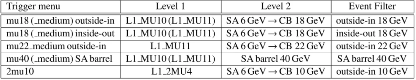
Tthreshold during 2011 with the change of the L1 seed from the L1 MU10 to L1 M11 as mentioned before. The mu22 medium outside-in trigger is used for the isolated muon trigger study. Table 1 shows the sequence of the muon trigger chains used in this note.
The mu18 triggers cover the needs of most physics analyses, however physics analyses which benefit
3
from muon triggers with lower- p
Tthreshold use either di-muon triggers or muon triggers in combination with other triggers. Some examples of such triggers are given in Table 2.
Table 1: Sequence of the muon trigger chains used in this note. Trigger chains with a muon spec- trometer (an inner detector) track based algorithm at the EF are called “outside-in” (“inside-out”). The L1 MU10 trigger consists of a two (three) station coincidence trigger in the barrel (endcap) region, and the L1 MU11 trigger, composed of coincidences of hits from three stations in both barrel and endcap re- gions, seeds “medium” chains. The L1 MU11 trigger was not prescaled throughout the 2011 data taking period, whereas the L1 MU10 trigger was prescaled while luminosity was above 1.9
×10
33cm
−2s
−1. The p
Tcut applied at each step of the chain is also shown. At the Level 1 the number after MU in a chain name denotes the p
Tthreshold in GeV. The mu40 SA barrel is a muon spectrometer standalone trigger in the barrel region only. The 2mu10 trigger requires two independent muons at each step.
Trigger menu Level 1 Level 2 Event Filter
mu18 ( medium) outside-in L1 MU10 (L1 MU11) SA 6 GeV
→CB 18 GeV outside-in 18 GeV mu18 ( medium) inside-out L1 MU10 (L1 MU11) SA 6 GeV
→CB 18 GeV inside-out 18 GeV mu22 medium outside-in L1 MU11 SA 6 GeV
→CB 22 GeV outside-in 22 GeV mu40 ( medium) SA barrel L1 MU10 (L1 MU11) SA barrel 40 GeV SA barrel 40 GeV
2mu10 L1 2MU4 SA 6 GeV
→CB 10 GeV outside-in 10 GeV
Table 2: Summary of trigger menus and target physics analyses. The mu18 L1J10 trigger is the 18 GeV threshold muon trigger chains seeded by the L1 MU10 trigger in combination with a jet trigger at L1. The e10 mu6 trigger is the 6 GeV threshold muon trigger in the presence of the 10 GeV threshold electron trigger. The tau20 mu15 trigger is the combined trigger of the 20 GeV threshold tau trigger and the 15 GeV threshold muon trigger.
Trigger menu Target physics analyses mu18 ( medium) SM, Higgs, SUSY, exotics
2mu10 Higgs, SM di-bosons
mu18 L1J10 SUSY
e10 mu6 Higgs, SM di-bosons
tau20 mu15 Higgs, Z
→ττ4 Processing time
The processing times of HLT algorithms have been determined on computers equipped with Intel
RCore
TM2 Duo CPU E8400 with clock speed of 3.00 GHz running on raw data from the events selected by jet, tau or missing E
Ttriggers at a luminosity of about 3.1
×10
33cm
−2s
−1. In 2011 the computing nodes of the HLT consisted mainly of Intel
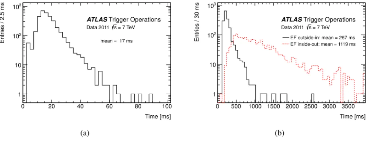
RHarpertown quad-core CPUs running at 2.5 GHz. For the timing measurement only one trigger chain, either mu18 medium inside-out or mu18 medium outside- in, was enabled to avoid a bias on the measurement due to the caching of the intermediate steps.
The processing time for the L2 CB chain is shown in Figure 2(a). The mean processing time was 17 ms, of which 63% was consumed by the L2 ID tracking part of the L2 CB algorithm, about 9% was used by the L2 SA and the rest was spent on data unpacking and decoding. Figure 2(b) shows
4
the corresponding times for the EF outside-in and inside-out algorithms. The average processing times were about 270 ms and 1120 ms for outside-in and inside-out algorithms, respectively. The composition of the processing time for the outside-in algorithm is: 65% for the SA algorithm, 29% for the CB algo- rithm and the remainder for unpacking and decoding of the data. The average number of muon RoIs per event seeding the mu18 chains was about 1.06. Due to a higher track multiplicity in the ID compared to the MS, especially in high occupancy events, the inside-out algorithm takes more processing time as it needs to extrapolate all the ID tracks in an RoI to the MS. For the 2012 data taking period, the inside-out algorithm is executed only if the outside-in algorithm could not find a muon candidate. In addition, a set of selection criteria for input ID tracks is under study in order to minimise the processing time by reducing the number of ID tracks to be extrapolated to the MS. The times were also measured with a data sample taken at a lower luminosity of about 1.0
×10
33cm
−2s
−1and are approximately 25% shorter compared to the sample taken at about 3.1
×10
33cm
−2s
−1.
The processing times of the HLT chains were well within the time restrictions allowing a stable trigger operation at luminosity of 3.0
×10
33cm
−2s
−1.
Time [ms]
0 20 40 60 80 100
Entries / 2.5 ms
1 10 102
103
mean = 17 ms
Trigger Operations ATLAS
= 7 TeV s Data 2011
(a)
Time [ms]
0 500 1000 1500 2000 2500 3000 3500
Entries / 30 ms
1 10 102
103
EF outside-in: mean = 267 ms EF inside-out: mean = 1119 ms
Trigger Operations ATLAS
= 7 TeV s Data 2011
(b)
Figure 2: Execution times of the HLT algorithms per RoI. The processing times of HLT algorithms have been determined on Intel
RCore
TM2 Duo CPU E8400 with clock speed of 3.00 GHz running on raw data from the events selected by jet, tau or missing E
Ttriggers at a luminosity of about 3.1
×10
33cm
−2s
−1. In 2011 the computing nodes of the HLT consisted mainly of Intel
RHarpertown quad-core CPUs run- ning at 2.5 GHz. The mean time of each algorithm is indicated in the legend. (a) is for the L2 combined reconstruction chain. (b) is for the EF trigger chains starting from a muon spectrometer track (outside- in) and an inner detector track (inside-out). The solid and dashed lines are for outside-in and inside-out chains, respectively.
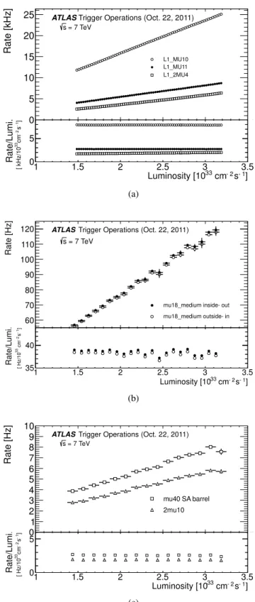
5 Trigger rate
Trigger rates have been measured during a run recorded on 22 October 2011 with a fill of 1332 proton bunches in 12 trains with 50 ns bunch spacing. Figure 3(a) shows the L1 trigger rates before prescale in terms of the luminosity. The L1 MU10 rate is about 15 kHz at a luminosity of 1.9 x 10
33cm
−2s
−1, and above this luminosity the L1 MU10 trigger was prescaled. The L1 MU11 rate is about 30% of the L1 MU10 rate due to the longer lever arm used to select muons above a p
Tthreshold in the toroidal magnetic field, allowing the L1 MU11 trigger to be unprescaled during the 2011 data taking period. The L1 trigger rate is dominated by triggers without associated offline muons (fake triggers). The overall fake trigger fraction at L1 was about 70%, of which most fake triggers originated from the endcap regions.
L1 2MU4 is a di-muon trigger which requires two muon candidate to each pass the L1 MU4 trigger.
5
Figure 3(b) shows rates of mu18 medium triggers for the same run. The trigger rate was about 110 Hz at 3.0
×10
33cm
−2s
−1. The inside-out algorithm shows a slightly higher trigger rate than the outside-in algorithm. Figure 3(c) shows the rates of other unprescaled muon triggers listed in Table 1, the medium- p
Tdi-muon trigger (2mu10) and the high-p
Tmuon spectrometer standalone trigger in the barrel region (mu40 medium SA barrel). The vertical error bars in each plot show the statistical errors. The observed trigger rates show a linear dependence on the luminosity. Table 3 summarises the trigger rates at an instantaneous luminosity of 3.0
×10
33cm
−2s
−1.
Table 3: The L1 (left) and EF (right) trigger rates of the main physics muon triggers and muon triggers in combination with other triggers at an instantaneous luminosity of 3.0
×10
33cm
−2s
−1.
Trigger Rate [kHz]
L1 MU10 24
L1 MU11 8
L1 2MU4 6
Trigger Rate [Hz]
mu18 medium outside-in 109 mu18 medium inside-out 111
mu40 medium SA barrel 7
2mu10 6
6 Data and Monte Carlo samples
In 2011 the ATLAS experiment recorded data from collisions of protons at 7 TeV centre-of-mass energy corresponding to an integrated luminosity of 5.3 fb
−1. With the mu18 medium trigger, 2.8 fb
−1of data are available after requiring good detector conditions. The amount of data used for subsequent analyses in this note vary depending on the purpose of the studies.
Optimal data-taking conditions for the detector system were required for an event to be accepted by the offline analysis. The events were then required to pass unprescaled single muon triggers. To ensure the event comes from a pp collision, at least one reconstructed primary vertex with more than two associated tracks was required, furthermore the z-position of the vertex was required to be located within 200 mm from the nominal interaction position.
In order to compare trigger performance between data and Monte Carlo (MC) simulation, MC sam- ples of Z bosons decaying to a muon pair were generated. The MC samples used were produced using the PYTHIA [5] event generator then processed through a GEANT4 [6] based simulation of the ATLAS detector [7]. The low-energy photons and neutrons generated from interactions in the cavern walls or beamline shielding were not simulated.
7 Muon selection
This note makes use of two classes of offline muons [1]:
Standalone (SA) muon:
The muon trajectory is reconstructed with the MS information only. The di- rection of flight and the impact parameter of the muon at the interaction point are determined by extrapolating the spectrometer track back to the beam line taking the energy loss of the muon in the calorimeters into account.
Combined (CB) muon:
Track reconstruction is performed independently in the ID and MS, and a track is formed from the successful combination of a MS track with an ID one. The momentum of the CB muon is calculated as the weighted average of the ID and the MS stand-alone momentum measurements.
6
1 1.5 2 2.5 3 3.5 0
1 2 3 4 5 6
] s-1 cm-2 Luminosity [1033
1 1.5 2 2.5 3 3.5
Rate [kHz]
0 5 10 15 20 25
L1_MU10 L1_MU11 L1_2MU4 ATLASTrigger Operations (Oct. 22, 2011)
= 7 TeV s
] s-1
cm-2
Luminosity [1033
1 1.5 2 2.5 3 3.5
Rate/Lumi. 0
5
]-1 s-2cm33[ kHz/10
0
(a)
-1 ] -2 s 33 cm Luminosity [10
1 1.5 2 2.5 3 3.5
Rate [Hz]
60 70 80 90 100 110 120
mu18_medium inside-out mu18_medium outside-in ATLASTrigger Operations (Oct. 22, 2011)
= 7 TeV s
-1 ]
-2 s
33 cm Luminosity [10
1 1.5 2 2.5 3 3.5
Rate/Lumi. 35
40
]-1 s-2 cm33[ Hz/10
(b)
1 1.5 2 2.5 3 3.5
Rate [Hz]
0 1 2 3 4 5 6 7
8 ATLAS
1 1.5 2 2.5 3 3.5
Rate [Hz]
01 23 45 67 89 10
mu40 SA barrel 2mu10 ATLASTrigger Operations (Oct. 22, 2011)
= 7 TeV s
] s-1
cm-2
Luminosity [1033
1 1.5 2 2.5 3 3.5
Rate/Lumi. 0
33-1-2 ] scm[ Hz/10 5 0
(c)
Figure 3: Trigger rates for a run recorded on 22 October 2011 with a fill of 1332 proton bunches in 12 trains with 50 ns bunch spacing. (a) shows the L1 trigger rates before prescale. The open circles are for L1 MU10 (2-station and 3-station coincidence triggers in RPC and TGC, respectively), the filled circles are for L1 MU11 (3-station coincidence trigger) and the open squares are for L1 2MU4. (b) shows the rates of two independent EF trigger algorithms operating at a p
Tthreshold of 18 GeV seeded by the L1 MU11 trigger, one starting from a muon spectrometer track (outside-in) and another starting from an inner detector track (inside-out). The filled circles and the open circles are for the mu18 medium inside-out and mu18 medium outside-in algorithms, respectively. In (c), the open triangles and open squares show trigger rates for 2mu10 and mu40 medium SA barrel, respectively. The lower part of each plot shows the ratio of rate to luminosity. The vertical error bars in each plot show the statistical errors.
7
All CB muons considered in the analysis must have a minimum number of hits in the silicon detectors.
Dead or missing sensors crossed by a track are counted as hits. Within the geometric acceptance of the TRT a successful extension of the muon trajectory into that detector is enforced by requirements on the numbers of associated good TRT hits and TRT outliers. TRT outliers appear in two forms in the track reconstruction, as a straw tube with a signal but not crossed by the near-by track or as a set of TRT measurements in the prolongation of a track which, however, failed to form a smooth trajectory with the pixel and SCT measurements. These quality cuts are put in place to suppress fake tracks and discriminate against muons from hadron decays. Combined muons which do not fulfil the ID hits requirements are rejected in the analysis.
In order to use muons within the acceptance of the L1 muon trigger system, muons were required to satisfy
|η|<2.4. For quantifying how well a muon track is isolated from other tracks,
ΣpTis defined as the sum of the p
Tof tracks with p
T >1 GeV found in the ID in a cone of
∆R=0.2 around the muon after subtracting the p
Tof the muon. If an isolated muon track is required,
ΣpTis demanded to be less than 10% of the p
Tof the muon.
In the tag-and-probe method, Z
→ µ+µ−decays were selected by requiring a pair of oppositely charged CB muons with a di-muon invariant mass near the mass of the Z boson. A CB muon has to pass the following cuts to be considered as a tag muon in offline analysis:
•
p
T >20 GeV;
• ΣpT/
p
T(tag)
<0.1 (isolation requirement as defined above);
•
to have an associated EF CB track with p
Tabove the threshold of unprescaled single muon triggers.
The separation between the muon and the EF CB track was required to satisfy
∆R <0.15 to be regarded as associated.
The probe muons and the tag-and-probe pairs were required to satisfy the following conditions:
• ΣpT/
p
T(probe)
<0.1 (isolation requirement as defined above);
•
the tag and the probe are oppositely charged;
• ∆φ >
2.0 (where
∆φis the azimuthal separation of the tag and the probe);
•
the invariant mass of the tag-and-probe pair is close to the nominal Z mass:
|m
Z−m
(tag,probe)|<10 GeV.
Using Monte Carlo samples [1], the fraction of probes that are not coming from Z decays was estimated to be less than 1% over the p
Trange of interest. The efficiency of a muon trigger chain with respect to offline isolated CB muons is the fraction of the probe muons which have an associated EF trigger track, that passed all the steps of the muon trigger chain, in a cone of
∆R=0.15 around the probe muon.
8 Trigger performance
8.1 The first level trigger
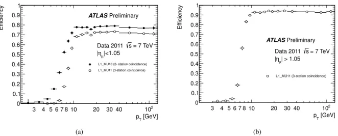
The performance of the L1 trigger seeding the unprescaled single muon trigger chains has been measured with the tag-and-probe method. Figures 4(a) and 4(b) show the dependence of efficiency on the p
Tof isolated offline CB muon for the L1 RPC trigger (
|η|<1.05) and the L1 TGC trigger (1.05
< |η| <2.4), respectively. In each figure, the vertical error bars show statistical errors. The amount of data used for the L1 RPC trigger efficiency measurement corresponds to 0.35 fb
−1taken after the last calibration per- formed on the RPC detectors during the 2011 data taking period. The L1 MU11 efficiency in the barrel region was about 2% lower before the last calibration. The L1 TGC trigger efficiency was measured with
8
[GeV]
pT
3 4 5 6 7 8 10 20 30 40 102
Efficiency
0 0.1 0.2 0.3 0.4 0.5 0.6 0.7 0.8 0.9 1
= 7 TeV s Data 2011
|<1.05 ηµ
|
ATLASPreliminary
L1_MU10 (2-station coincidence) L1_MU11 (3-station coincidence)
(a)
[GeV]
pT
3 4 5 6 7 8 10 20 30 40 102
Efficiency
0 0.1 0.2 0.3 0.4 0.5 0.6 0.7 0.8 0.9 1
ATLASPreliminary = 7 TeV s Data 2011
| > 1.05 ηµ
|
L1_MU11 (3-station coincidence)
(b)
Figure 4: L1 trigger efficiency with respect to isolated offline combined muons for (a) the barrel region and (b) the endcap regions. In the barrel region, L1 MU10 is the two-station coincidence trigger shown as the filled circles. The open circles are for L1 MU11 which is the three-station coincidence trigger. The tag-and-probe method with Z
→ µ+µ−events was used to derive efficiencies. The efficiencies include geometric acceptance of the detectors. The vertical error bars in each figure represent statistical errors.
The amount of data used for the L1 RPC trigger efficiency measurement corresponds to 0.35 fb
−1taken after the last calibration performed on the RPC detectors during the 2011 data taking period. The data corresponding to an integrated luminosity of 2.8 fb
−1were used for the L1 TGC efficiency measurement.
data corresponding to an integrated luminosity of 2.8 fb
−1taken after the run in which the L1 MU10 trig- ger was first prescaled. For the RPC trigger, e
fficiencies of both the L1 MU10 and L1 MU11 triggers are shown. Due to the smaller geometric coverage of the additional chambers required to form three-station coincidence triggers and hit efficiencies of the additional chambers, the L1 MU11 trigger shows about 6% lower efficiency compared to the L1 MU10 trigger. In the endcap regions the L1 MU11 trigger effi- ciency is shown. In both the barrel and endcap regions, the efficiency depends on the charge (q) and the
ηof a muon, as the bending direction in the toroidal magnetic field depends on the product q
×η. Aroundthe barrel and endcap boundaries, if q
×ηof a muon is negative (positive), the muon pointing to TGC (RPC) at the interaction point bends towards RPC (TGC). The difference in efficiency between muons with positive and negative q
×ηbecomes smaller as the p
Tof muons increases. Also in the very high- p
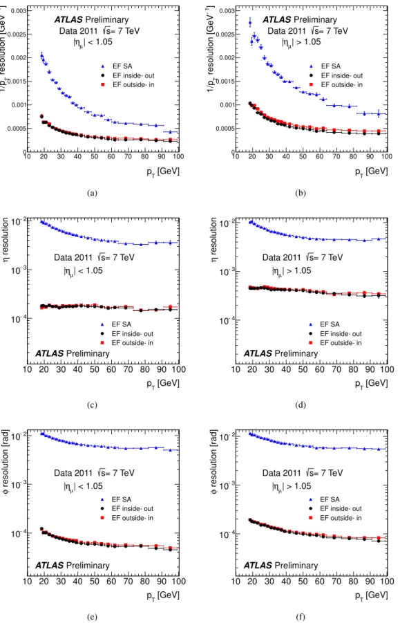
Tregion, the efficiency starts to decrease due to radiation from muons. The efficiency in the plateau region is affected by these effects. Table 4 summarises these average plateau efficiencies and p
Tvalues at which efficiency becomes 95% (90%) of the average plateau efficiencies. The p
Tcut was changed by 0.1 GeV steps to find the corresponding p
Tvalues. The L1 triggers become fully efficient well below 18 GeV in both the barrel and endcap regions. The average plateau efficiency of the L1 MU11 trigger is 0.725 and 0.935 for the barrel and the endcap regions, respectively. The statistical uncertainty on the average plateau efficiencies is of the order of 0.1% or less, and the efficiency includes the geometric acceptance of the detectors. The maximum deviation of the efficiency in a p
Tbin above 20 GeV from the average plateau efficiencies are about 0.015 and 0.009 in the barrel and endcap regions, respectively.
9
Table 4: The average plateau efficiency and p
Tvalues at which the efficiency becomes 95% (90%) of the average plateau efficiencies. The p
Tcut was changed by 0.1 GeV steps to find the corresponding p
Tvalues. The statistical uncertainty on the average plateau efficiencies is of the order of 0.1% or less, and the efficiency includes the geometric acceptance of the trigger detectors. The maximum deviation of the efficiency in a p
Tbin above 20 GeV from the average plateau efficiencies are about 0.015 and 0.009 in the barrel and endcap regions, respectively.
Trigger Average plateau e
fficiency p
Tat 95% (GeV) p
Tat 90% (GeV)
L1 MU10 (Barrel) 0.785 11.2 9.5
L1 MU11 (Barrel) 0.725 11.7 10.7
L1 MU11 (Endcaps) 0.935 9.3 8.7
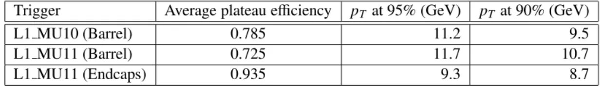
8.2 The second level trigger
The resolution of the L2 track parameters associated to the mu18 medium chains has been measured with muons from Z boson decays. Distributions of the residuals between the L2 and offline muon track parameters (1/ p
T,
ηand
φ) were reconstructed in bins ofp
T, then Gaussian fits were performed to extract the widths,
σ, of the residual distributions as a function of p
T. The inverse-p
Tof L2 SA and L2 CB muons were compared to those of the offline CB muons to calculate residuals. As the
ηand
φof L2 SA muons are defined at the MS, offline track parameters of SA were used to compute
ηand
φresiduals of L2 SA tracks. On the other hand,
ηand
φresiduals of L2 CB muons were derived with
ηand
φof the offline CB muons. A minimum p
Tcut of 10 GeV was applied to exclude the p
Tregion where there are not enough probe muons from Z decays to extract the parameters.
The inverse-p
Tresidual widths of L2 SA and L2 CB muons,
σ((1
/p
T)
L2−(1
/p
T)
offline), are shown in Figure 5(a) for the barrel region and in Figure 5(b) for the endcap regions as a function of the offline muon p
T. The L2 CB algorithm improves the resolution compared to the L2 SA algorithm by using additional measurements from tracks reconstructed in the ID, particularly in the low- p
Tregion. Although the improvement of the resolutions by the L2 CB algorithm in the barrel region becomes smaller as the p
Tof the muon increases, this will not affect the performance of the 18 GeV p
Tthreshold trigger. The
ηresidual widths,
σ(
ηL2−ηoffline), are shown in Figure 5(c) for the barrel region and in Figure 5(d) for the endcap regions in terms of the offline muon p
T. The dependence of the
φresidual widths,
σ(φL2−φoffline), on offline muon p
Tis shown in Figure 5(e) for the barrel region and in Figure 5(f) for the endcap regions.
The L2 CB algorithm uses the
ηand
φdetermined by the L2 ID tracking, thus the p
Tdependence of
ηand
φresolutions reflects performance of the L2 ID tracking. The errors on the resolutions are the value of
σobtained from the Gaussian fit in each p
Tslice. The p
Tresolution in the endcaps are worse than the one in the barrel due to the complex magnetic field in the endcap regions. The
ηand
φresolutions achieved were adequate to combine a muon SA track with ID track associated with the muon SA track.
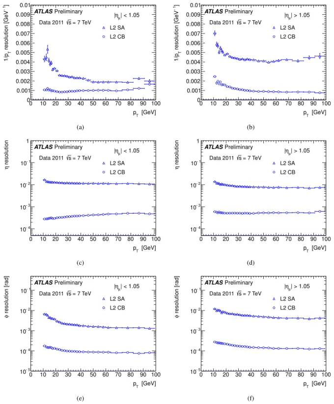
8.3 The event filter
In order to examine the performance of the EF algorithms, the residuals between the EF and offline muon track parameters (1/p
T,
ηand
φ) were evaluated in bins ofp
T, then the widths of the residual distributions were extracted in each bin with a Gaussian fit. The track parameters of EF SA and EF CB muons were compared to those of offline CB muons to calculate residuals. A minimum p
Tcut of 18 GeV was applied to offline CB muons for studying relative resolutions of EF tracks reconstructed in mu18 medium chains.
The inverse-p
Tresidual widths of EF SA, EF outside-in and EF inside-out tracks,
σ((1/p
T)
EF −(1
/p
T)
offline), are shown in Figure 6(a) for the barrel region and in Figure 6(b) for the endcap regions as a function of the offline muon p
T. The improvement in p
Tresolution, particularly at lower-p
T, resulting
10
[GeV]
pT
0 10 20 30 40 50 60 70 80 90 100 ]-1 resolution [GeV T1/p
0 0.001 0.002 0.003 0.004 0.005 0.006 0.007 0.008 0.009
0.01 ATLASPreliminary
L2 SA L2 CB = 7 TeV
s Data 2011
| < 1.05 ηµ
|
(a)
[GeV]
pT
0 10 20 30 40 50 60 70 80 90 100 ]-1 resolution [GeV T1/p
0 0.001 0.002 0.003 0.004 0.005 0.006 0.007 0.008 0.009
0.01 ATLASPreliminary
L2 SA L2 CB = 7 TeV
s Data 2011
| > 1.05 ηµ
|
(b)
[GeV]
pT
0 10 20 30 40 50 60 70 80 90 100
resolutionη
10-4
10-3
10-2
10-1
1 ATLASPreliminary
L2 SA L2 CB = 7 TeV
s Data 2011
| < 1.05 ηµ
|
(c)
[GeV]
pT
0 10 20 30 40 50 60 70 80 90 100
resolutionη
10-4
10-3
10-2
10-1
1 ATLASPreliminary
L2 SA L2 CB = 7 TeV
s Data 2011
| > 1.05 ηµ
|
(d)
[GeV]
pT
0 10 20 30 40 50 60 70 80 90 100
resolution [rad]φ
10-5
10-4
10-3
10-2
10-1
ATLASPreliminary
L2 SA L2 CB = 7 TeV
s Data 2011
| < 1.05 ηµ
|
(e)
[GeV]
pT
0 10 20 30 40 50 60 70 80 90 100
resolution [rad]φ
10-5
10-4
10-3
10-2
10-1
ATLASPreliminary
L2 SA L2 CB = 7 TeV
s Data 2011
| > 1.05 ηµ
|
(f)
Figure 5: Resolutions of the inverse p
T,
ηand
φtrack parameters of the L2 SA and L2 CB algorithms, measured with the muons from Z
→ µ+µ−sample, are shown as a function of offline muon p
Tin the barrel and endcap regions. The triangles and the circles are for L2 SA and L2 CB muons, respectively.
(a) and (b) show 1/p
Tresolutions in the barrel and endcaps regions, respectively. (c) and (d) show
ηresolutions in the barrel and endcaps regions, respectively. (e) and (f) shows
φresolutions in the barrel and endcaps regions, respectively. The vertical error bars on the resolutions are the value of
σobtained from the Gaussian fit in each p
Tslice. The amount of data used for the resolution study corresponds to an integrated luminosity of about 2 fb
−1.
11
from the inclusion of ID track information is evident from a comparison between the EF SA and EF CB algorithms. The
ηresidual widths,
σ(ηEF−ηoffline), are shown in Figure 6(c) for the barrel region and in Figure 6(d) for the endcap regions in terms of the offline muon p
T. The dependence of
φresidual widths,
σ(φEF−φoffline), on offline muon p
Tis shown in Figure 6(e) for the barrel region and in Figure 6(f) for the endcap regions. The errors on the resolutions are the value of
σobtained from the Gaussian fit in each p
Tslice. These figures illustrate the good agreement between the track parameters calculated online and offline. The level of agreement is similar for both inside-out and outside-in algorithms.
12
[GeV]
pT 10 20 30 40 50 60 70 80 90 100
]-1 resolution [GeV T1/p
0 0.0005 0.001 0.0015 0.002 0.0025 0.003
ATLASPreliminary
= 7 TeV s Data 2011
| < 1.05 ηµ
|
EF SA EF inside-out EF outside-in
(a)
[GeV]
pT 10 20 30 40 50 60 70 80 90 100
]-1 resolution [GeV T1/p
0 0.0005 0.001 0.0015 0.002 0.0025 0.003
ATLASPreliminary
= 7 TeV s Data 2011
| > 1.05 ηµ
|
EF SA EF inside-out EF outside-in
(b)
[GeV]
pT
10 20 30 40 50 60 70 80 90 100
resolutionη
10-4
10-3
10-2
= 7 TeV s Data 2011
| < 1.05 ηµ
|
ATLASPreliminary
EF SA EF inside-out EF outside-in
(c)
[GeV]
pT
10 20 30 40 50 60 70 80 90 100
resolutionη
10-4
10-3
10-2
= 7 TeV s Data 2011
| > 1.05 ηµ
|
ATLASPreliminary
EF SA EF inside-out EF outside-in
(d)
[GeV]
pT
10 20 30 40 50 60 70 80 90 100
resolution [rad]φ
10-4
10-3
10-2
= 7 TeV s Data 2011
| < 1.05 ηµ
|
ATLASPreliminary
EF SA EF inside-out EF outside-in
(e)
[GeV]
pT
10 20 30 40 50 60 70 80 90 100
resolution [rad]φ
10-4
10-3
10-2
= 7 TeV s Data 2011
| > 1.05 ηµ
|
ATLASPreliminary
EF SA EF inside-out EF outside-in
(f)
Figure 6: Resolutions of the inverse p
T,
ηand
φtrack parameters of the EF standalone and combined algorithms, measured with the muons from Z
→ µ+µ−sample, are shown as a function of the offline muon p
T. The triangles are for EF SA, and the circles and the squares are for the two independent EF trigger algorithms, one starting from the muon spectrometer track (outside-in) and another starting from the inner detector track (inside-out), respectively. (a) and (b) show 1
/p
Tresolutions in the barrel and endcaps, respectively. (c) and (d) show
ηresolutions in the barrel and endcaps, respectively. (e) and (f) show
φresolutions in the barrel and endcaps, respectively. The errors on the resolutions are the value of
σobtained from the Gaussian fit in each p
Tslice. The amount of data used for the resolution study corresponds to an integrated luminosity of about 2 fb
−1.
13
8.4 Trigger e ffi ciency
Efficiencies of the mu18 medium trigger chains with respect to isolated offline combined muons have been evaluated with the tag-and-probe method using Z
→µ+µ−events. The amount of data used corre- sponds to an integrated luminosity of 2.8 fb
−1collected after the run in which the L1 MU10 trigger was first prescaled. Figure 7 shows measured efficiencies of data and MC in the barrel and endcap regions as a function of muon p
Tfor the outside-in and the inside-out algorithms. The vertical error bars and the vertical width of rectangles in each plot show the statistical errors. Table 5 summarises the average plateau efficiencies and p
Tvalues at which the efficiency becomes 95% (90%) of the average plateau efficiency. The p
Tcut was changed by 0.1 GeV steps to find the corresponding p
Tvalues. The triggers are fully efficient at p
Tof 20 GeV where an offline analysis can place a minimum p
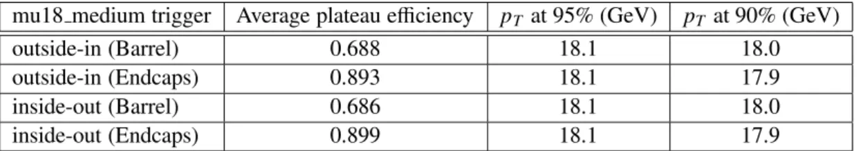
Tcut. Both the outside-in and the inside-out algorithms show similar efficiencies in the barrel and endcap regions. The overall efficiency for data in the plateau region is well described by the Monte Carlo simulation and the turn-on region is modelled reasonably well. The ratios are slightly below 1 in the barrel region due to non-optimal modelling in the simulation of efficiencies and conditions of the RPC detectors during the 2011 data taking period.
Table 5: The average plateau efficiency and p
Tvalues at which the efficiency becomes 95% (90%) of the average plateau efficiencies. The p
Tcut was changed by 0.1 GeV steps to find the corresponding p
Tvalues. The statistical uncertainty on the average plateau efficiencies is of the order of 0.1% or less, and the efficiencies include the geometric acceptance of the trigger detectors. The maximum deviation of the efficiency in a p
Tbin above 20 GeV from the average plateau efficiencies are about 0.036 (0.039) and 0.013 (0.008) in the barrel and endcap regions for the outside-in (inside-out) algorithm, respectively.
mu18 medium trigger Average plateau e
fficiency p
Tat 95% (GeV) p
Tat 90% (GeV)
outside-in (Barrel) 0.688 18.1 18.0
outside-in (Endcaps) 0.893 18.1 17.9
inside-out (Barrel) 0.686 18.1 18.0
inside-out (Endcaps) 0.899 18.1 17.9
Figure 8 show the efficiencies of the mu18 medium trigger chains in terms of the number of interac- tions per bunch crossing, i.e. calculated from the luminosity assuming an inelastic proton-proton cross section of 71.5 mb. for muons with p
T >20 GeV. The data were collected during the LHC operation at
β∗=1.0 m corresponding to an integrated luminosity of 1.9 fb
−1. The efficiencies include the geo- metric acceptance of the L1 trigger chambers in the barrel and endcap regions. The vertical error bars in each plot show the statistical errors. Efficiencies of both the outside-in and the inside-out mu18 medium chains show a weak dependence on event pile-up conditions due to the degradation of L2 ID tracking performance in high pile-up events. The loss of efficiency at L2 ID tracking is about 0.1% per unit increase in the number of reconstructed vertices.
14
[GeV]
pT
10 20 30 40 50 60 70 80 102
Efficiency
0 0.1 0.2 0.3 0.4 0.5 0.6 0.7 0.8 0.9 1
Data MC ATLASPreliminary
= 7 TeV s Data 2011
| < 1.05 ηµ
|
mu18 medium outside-in
[GeV]
pT
10 20 30 40 50 60 70 80 102
Data/MC
0.95 1 1.050
(a)
[GeV]
pT
10 20 30 40 50 60 70 80 102
Efficiency
0 0.1 0.2 0.3 0.4 0.5 0.6 0.7 0.8 0.9 1
Data MC ATLASPreliminary
= 7 TeV s Data 2011
| > 1.05 ηµ
|
mu18 medium outside-in
[GeV]
pT
10 20 30 40 50 60 70 80 102
Data/MC
0.95 1 1.050
(b)
[GeV]
pT
10 20 30 40 50 60 70 80 102
Efficiency
0 0.1 0.2 0.3 0.4 0.5 0.6 0.7 0.8 0.9 1
Data MC ATLASPreliminary
Data 2011
| < 1.05 ηµ
|
mu18 medium inside-out
[GeV]
pT
10 20 30 40 50 60 70 80 102
Data/MC
0.95 1 1.050
(c)
[GeV]
pT
10 20 30 40 50 60 70 80 102
Efficiency
0 0.1 0.2 0.3 0.4 0.5 0.6 0.7 0.8 0.9 1
Data MC ATLASPreliminary
Data 2011
| > 1.05 ηµ
|
mu18 medium inside-out
[GeV]
pT
10 20 30 40 50 60 70 80 102
Data/MC
0.95 1 1.050
(d)
Figure 7: Efficiencies of the mu18 medium trigger chains in terms of the offline reconstructed muon p
T. In the upper part of each plot, the circles and the rectangles show data and MC, respectively. The lower part of each plot shows ratio of data efficiencies to those of the MC. The tag-and-probe method with Z
→ µ+µ−events was used to derive efficiencies. The vertical error bars and the vertical width of the rectangles in each plot show the statistical errors. (a) and (b) show efficiencies of the triggers with the muon spectrometer track based algorithm at EF (outside-in) in the barrel and endcap regions, respectively. (c) and (d) show the trigger e
fficiencies using the inner detector track based algorithm at EF (inside-out) in the barrel and endcap regions, respectively. The efficiencies includes the geometric acceptance of the L1 trigger chambers. The amount of data used for the trigger efficiency measurement corresponds to 2.8 fb
−1.
15
interactions per bunch crossing
0 5 10 15 20 25
Efficiency
0.3 0.4 0.5 0.6 0.7 0.8 0.9 1 1.1
| > 1.05 ηµ
mu18_medium outside-in | | < 1.05 ηµ
mu18_medium outside-in |
ATLASPreliminary
= 7 TeV s Data 2011
(a)
interactions per bunch crossing
0 5 10 15 20 25
Efficiency
0.3 0.4 0.5 0.6 0.7 0.8 0.9 1 1.1
| > 1.05 ηµ
mu18_medium inside-out | | < 1.05 ηµ
mu18_medium inside-out |
ATLASPreliminary
= 7 TeV s Data 2011
(b)
Figure 8: The trigger efficiencies in the plateau region ( p
T >20 GeV) are shown as a function of interactions per bunch crossing for data collected during LHC operation at
β∗=1.0 m. The tag-and-probe method using Z
→µ+µ−events was used to derive these efficiencies. (a) and (b) are for mu18 medium triggers with the muon spectrometer track based algorithm at EF (outside-in) and with the inner detector track based algorithm at EF (inside-out), respectively. The circles are for barrel and the triangles are for endcap regions, respectively. The difference of the efficiencies in the barrel and endcap regions is due to the geometric acceptance of the L1 trigger chambers. The vertical error bars in each figure represent the statistical errors only. The amount of data used corresponds to 1.9 fb
−1.
8.5 Scale factors and application to physics analyses
In order to account for the mis-modelling of the trigger performance in simulated samples, scale factors (SF) are computed as follows,
SF
=1
−QNn=1
(1
−Data,n) 1
−QNn=1