JHEP01(2016)076
Published for SISSA by Springer
Received: November 9, 2015 Accepted: December 22, 2015 Published: January 13, 2016
Cancellation of Glauber gluon exchange in the double Drell-Yan process
Markus Diehl,a Jonathan R. Gaunt,a,1 Daniel Ostermeierb Peter Pl¨oßlb and Andreas Sch¨aferb
aDeutsches Elektronen-Synchroton DESY, 22603 Hamburg, Germany
bInstitut f¨ur Theoretische Physik, Universit¨at Regensburg, 93040 Regensburg, Germany
E-mail: markus.diehl@desy.de,jgaunt@nikhef.nl, Daniel.Ostermeier@physik.uni-regensburg.de, Peter.Ploessl@physik.uni-regensburg.de, Andreas.Schaefer@physik.uni-regensburg.de
Abstract: An essential part of any factorisation proof is the demonstration that the exchange of Glauber gluons cancels for the considered observable. We show this cancellation at all orders for double Drell-Yan production (the double parton scattering process in which a pair of electroweak gauge bosons is produced) both for the integrated cross section and for the cross section differential in the transverse boson momenta. In the process of constructing this proof, we also revisit and clarify some issues regarding the Glauber cancellation argument and its relation to the rest of the factorisation proof for the single Drell-Yan process.
Keywords: Hadronic Colliders, QCD Phenomenology ArXiv ePrint: 1510.08696
1Present address: Nikhef Theory Group and VU University Amsterdam, De Boelelaan 1081, 1081 HV Amsterdam, The Netherlands
JHEP01(2016)076
Contents
1 Introduction 2
2 Overview of the factorisation proof 3
2.1 Overall strategy 4
2.2 Scaling of soft momenta 17
2.3 Approximations for soft gluons 19
3 Glauber cancellation for one-gluon exchange 21
3.1 Scope and general method 21
3.2 Grammer-Yennie approximation and rearrangement of terms 23
3.3 Explicit calculations in a simplified setting 24
3.3.1 Double box graph 26
3.3.2 Lightlike Wilson lines 27
3.3.3 Alternative momentum routings 30
3.3.4 Wilson lines with finite rapidity 32
3.3.5 Gauge boson vertex correction 35
3.4 General prescription for avoiding the Glauber region 36
3.5 Limitations of the present method 37
4 All-order proof of Glauber gluon cancellation 38
4.1 Light-cone perturbation theory (LCPT) 41
4.2 Derivation of LCPT from covariant perturbation theory 42
4.3 Absence of pinched poles in the Glauber region 43
4.3.1 Single Drell-Yan 43
4.3.2 Double Drell-Yan 47
4.3.3 Including longitudinally polarised collinear gluons 49 4.3.4 Independence of the remainderR on partitioning of soft vertices 49
5 Summary 52
A Evaluation of Feynman integrals in light-cone coordinates 53 B Alternative approach to the double scattering collinear factor 53
C Timelike Wilson lines 55
JHEP01(2016)076
1 Introduction
As the LHC continues to run after its energy upgrade, hopes are high that signals for physics beyond the Standard Model will show up in the coming years. To identify such signals and to understand their nature will be challenging for experiment and theory. This provides strong motivation to strive for a detailed and quantitative understanding of the final state in high-energy proton-proton collisions. Steady progress in perturbative calculations al- lows for increasing precision in describing the final state of a single parton-level scattering.
However, much remains to be understood even at the conceptual level for multiple hard interactions, where several parton-level scatters occur in one proton-proton collision. While such multiple interactions are power suppressed in sufficiently inclusive cross sections, they are unsuppressed in specific regions of phase space [1]. Moreover, their importance grows with increasing collision energy. Since many search channels for new physics involve high multiplicity, a thorough understanding of multiple hard scattering is highly desirable. Re- cent years have seen considerable progress, from theory to phenomenology to experimental studies, as is for instance documented in the proceedings [2–5].
The theory for single hard scattering in proton-proton collisions rests on factorisation formulae, which describe the cross section in terms of parton distributions, hard-scattering cross sections at parton level, and possibly other quantities like soft factors. Substantial effort has gone into proving these formulae to all orders of perturbation theory in QCD, see e.g. [6–8] for comprehensive accounts. A crucial part of such proofs is to cast the exchange of soft gluons between the two colliding protons into a form consistent with the factorisation formula. In particular kinematics, which is referred to as the Glauber region and which essentially describes small-angle parton-parton scattering, the approximations required to achieve such a form break down. Factorisation therefore only holds if the net effect of all Glauber gluon exchanges cancels in the observable considered. A prominent example where such a cancellation fails to occur (and factorisation is strongly violated) is hard diffraction [9, 10]. Observables in Drell-Yan production for which Glauber gluon exchange breaks factorisation are discussed in [11,12].
Factorisation formulae can also be written down for multiple hard scattering, where multi-parton distributions appear instead of the familiar single-parton distributions. To- gether with model assumptions connecting these multi-parton distributions with their single-parton counterparts, this forms the basis of most phenomenological investigations, see for instance [13–45]. To put this framework on a more solid footing, it is necessary to understand whether factorisation actually holds for multiple hard scattering. Several pieces of evidence pointing towards a positive answer have been given in [1, 46, 47], but the issue of Glauber gluons in this context has not been analysed yet. It is the purpose of the present paper to fill this gap. We limit ourselves to double hard scattering and more specifically to the double Drell-Yan process, i.e. to the production of two electroweak gauge bosons. To the best of our knowledge, the cancellation of Glauber gluon exchange in single hard scattering has also been established only for Drell-Yan production [8,48–50]. We will show that the proof given in [8] can indeed be adapted to the double Drell-Yan process. In doing so, we will revisit and clarify some subtle issues in the single Drell-Yan case.
JHEP01(2016)076
The most commonly used form of factorisation involves parton distributions integrated over transverse parton momenta, often called “collinear” distributions. Correspondingly, the net transverse momentum of the particles produced in a hard-scattering subprocess is then integrated over in the cross section formula. A different factorisation formalism uses transverse-momentum dependent parton distributions (TMDs). It allows one for in- stance to compute the transverse-momentum spectrum of the gauge boson produced in the Drell-Yan process in the region where that transverse momentum is small compared to the boson invariant mass. TMD factorisation for hadron-hadron collisions has only been established for cases where the particles produced in the hard scattering are colourless, i.e. for the production of electroweak gauge bosons and Higgs particles. For final states involving hadrons, problems related to gluon exchange in the Glauber region have so far prevented the formulation of TMD factorisation [51]. Under the restriction to colourless final states, our proof of Glauber gluon cancellation for double hard scattering holds in both the collinear and TMD cases. As already noted for single DY production in [8], such a proof is no more complicated (if not simpler) in the TMD framework than for collinear factorisation, and we treat both cases together in this paper. A possible extension to fi- nal states involving hadrons, which is of obvious phenomenological relevance, must await further work.
This paper is organised as follows. In the next section we give an account of the overall logic and status of a factorisation proof for the double Drell-Yan process, in close analogy to the single Drell-Yan case. Section3analyses one-gluon exchange in a toy model, with explicit calculations illustrating the role of complex contour deformation in avoiding contributions from the Glauber region. Within this toy model we show how the exchange of a single Glauber gluon cancels in the cross section. In section4 we present an all-order proof, following the work in [8, 50] on single Drell-Yan production, where an essential tool is light-cone time ordered perturbation theory. We summarise our main results in section 5.
2 Overview of the factorisation proof
In this section we give a broad overview over the different steps of the factorisation proof for double hard scattering with colourless final state particles. For definiteness, we consider double Drell-Yan production,p+p→V1+V2+X, where V1 andV2 are electroweak gauge bosons and X is the unobserved hadronic final state. Although many of the steps do not directly concern the main topic of this work, namely the cancellation of Glauber gluon exchange, we find it important to exhibit the interplay of this part of the proof with the other steps, which need to be taken in a consistent order.
Several parts of the factorisation proof have been elaborated in [1] or [47], but others still require further work in our opinion. Many elements of the proof are the same for TMD and collinear factorisation, so that the discussion can conveniently treat both cases in parallel. We largely follow the factorisation proof for single Drell-Yan production as given in chapter 14 of [8], with some modifications that we will point out.
JHEP01(2016)076
2.1 Overall strategy
1. Power counting. Both collinear and TMD factorisation are based on a power ex- pansion in a small parameter Λ/Q. Here Qis the hard scale of the process, whereas Λ represents small kinematic quantities and the scale of nonperturbative QCD inter- actions. The terms “leading” and “dominant” refer to the limit of small Λ/Q.
In double Drell-Yan production, Q is given by the invariant masses of the two pro- duced bosons (which we treat as being of the same order). For collinear factorisation there is no kinematic scale of size Λ, whereas for TMD factorisation the transverse momenta of the bosons are counted to be of order Λ. This doesnot mean that TMD factorisation is limited to transverse momenta in the nonperturbative region; what counts is that they are small compared with the hard scale of the process. Since Λ/Q is the parameter used to quantify the accuracy of the final factorisation formula, Λ is to be taken as the largest of all scales counted as “small” andQas the smallest of all scales counted as “large”.
2. Dominant graphs and regions. Following the analysis of Libby and Sterman [52, 53], one identifies the dominant regions of loop integration for each individual graph that contributes to the cross section. These regions are characterised by the mo- menta of internal lines being either hard, soft (which includes the Glauber region), or collinear to an external direction. They correspond to pinch singularities of the graph when all quantities of order Λ (masses and transverse momenta) are set to zero. For double Drell-Yan production there are just two collinear directions, given by the incoming protons. Within collinear factorisation, unobserved jets in the final state provide additional directions for collinear lines, but they disappear in the final result. (In TMD factorisation, production of additional jets is power suppressed due to the requirement of small transverse momentum for the produced gauge bosons.) For each leading momentum region, a graph can be organised into subgraphs con- taining only hard, soft or collinear lines. Dimensional analysis shows how these subgraphs can be connected in order to give a leading contribution. In this con- text, different roles are played by gluons with transverse or longitudinal polarisation (respectively having a polarisation vector that is approximately transverse or approx- imately proportional to the gluon momentum). A collinear and a hard subgraph must be connected by the minimum number of quarks1 or transverse gluons necessary for the process, whereas there can be any number of longitudinal gluons. Between a collinear and a soft graph there can be any number of soft gluons. We only consider soft subgraphs that couple to at least two different collinear graphs; soft subgraphs connecting to a single collinear graph are treated as a part of that graph. Soft gluons coupling to a hard subgraph are power suppressed.
For our further discussion we introduce light-cone coordinates, a± = (a0 ±a3)/√ 2 for each four-vector and denote its transverse components asa= (a1, a2). The com- ponents of the full vector are given as (a+, a−,a). We choose a coordinate system in
1For ease of language, we use the term “quarks” to denote both quarks and antiquarks.
JHEP01(2016)076
the overall c.m. frame where both incoming protons have zero transverse momentum, with one proton moving fast to the right and the other fast to the left. The typical size of momenta is then
l∼(Q, Q, Q) for hard lines,
l∼(Q,Λ2/Q,Λ) for right-moving collinear lines,
l∼(Λ2/Q, Q,Λ) for left-moving collinear lines. (2.1) Virtualities are thus of order Q2 for hard lines and of order Λ2 for collinear lines.
We note that in low-order graphs, hard momenta may have small or zero transverse components, which does however not affect the general analysis. Soft momenta have all components of order Λ or smaller. As we will discuss in section 2.2, there are important differences whether soft momentum components are of order Λ or Λ2/Q.
The analysis described here is based on Feynman graphs in perturbation theory. It is understood that in the final factorisation formula, quantities that involve lines with virtuality Λ2 or less (i.e. collinear or soft lines) will be represented by hadronic matrix elements of quark and gluon operators, which are meaningful beyond pertur- bation theory.
After these preliminaries, we can now specify the dominant graphs for double Drell- Yan production.
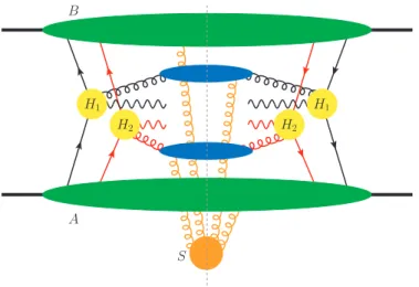
(a) For TMD factorisation, the dominant graphs are as shown in figure1. They have the same structure as for single Drell-Yan production, except that there are two distinct hard-scattering subgraphs on either side of the final-state cut. For ease of notation, we group the hard subgraphs such that Hi (i = 1,2) comprises the two subgraphs (on either side of the final-state cut) that produce the gauge boson Vi. There are exactly four quark lines entering each subgraph Hi. We denote the collinear subgraph with right-moving lines byAand the one with left-moving lines byB. Each of them has four external quark lines and is related to a double-parton distribution that appears in the final factorisation formula.
We note that the soft factorS may consist of several connected components. As mentioned above, each of these components must couple to bothAand B. The simplest connected subgraphs of S consist of one gluon directly connecting the two collinear graphs.
(b) The dominant graphs in collinear factorisation are more complicated since each of the two hard scatters can produce additional jets, which are part of the unobserved hadronic final stateXin the cross section. These additional collinear factors in the final state can further couple to the soft subgraph, as shown in figure2. A series of arguments is needed to convert this to two hard-scattering graphs with cut parton lines in the final state, as in figure3. The arguments are the same as for the single Drell-Yan process. We will review them in a separate publication.
JHEP01(2016)076
H1 S
H2 H2
H1
B
A
Figure 1. Dominant graphs for double Drell-Yan production, p+p → V1+V2+X, in TMD factorisation. A and B denote collinear subgraphs, S the soft subgraph, and H1, H2 the hard subgraphs.
S H1
H2 H2
H1
B
A
Figure 2. Dominant graph for double Drell-Yan production, p+p→ V1+V2+X, in collinear factorisation, with one unobserved jet produced by each hard scatter. Not shown for the sake of clarity are additional longitudinal gluons that can be exchanged between each pair of a hard and a collinear subgraph.
At higher orders in αs, incoming quarks in a hard graph can be replaced by gluons with transverse polarisation. The four partons with physical polarisation in each collinear factor thus can be different combinations of quarks and gluons.
For brevity we will call these “physical partons”.
(c) While the reactionp+p→V1+V2+X can proceed by double hard scattering (double parton scattering, DPS), two gauge bosons can also be produced in a single hard scattering (single parton scattering, SPS). In TMD factorisation, SPS and DPS have the same power behaviour in Λ/Q whereas in collinear factorisation SPS is enhanced over DPS by a factorQ2/Λ2. (On the other hand, due to a larger flux of incoming partons, DPS is generically enhanced over SPS at smallQ2/s, wheresis the squaredppc.m. energy.) There are also interference
JHEP01(2016)076
S H1
B
A
H2
Figure 3. Simplification of figure2 after a series of approximations. Again, an arbitrary number of longitudinal gluons can be exchanged between each hard and collinear subgraph.
terms between SPS and DPS, which have the same power behaviour as DPS for both TMD and collinear factorisation. For details we refer to section 2.4 of [1].
As discussed in sections 5.2.3 and 5.3 of [1], certain graphs can contribute to both SPS and DPS in different momentum regions. (An example is graph b in figure 9 below.) The existing factorisation formulae for DPS extend into the SPS region and vice versa, so that there is a double counting problem. This problem has been discussed in [46, 54–57], but in our opinion it has not been solved in a satisfactory way.
3. Approximations. In each dominant momentum region of a graph, one makes ap- propriate approximations. As discussed in section 10.4.2 of [8], these can be grouped into different types:
(a) Kinematics. For collinear lines entering a hard subgraph one keeps only large light-cone components, neglecting small light-cone components and transverse components. A right-moving momentum ℓenteringHi is thus replaced by
ℓˆ= (ℓ+,0,0). (2.2)
A small rescaling of the large components can be made so as to have exact momentum conservation in the hard subgraph. In hard subgraphs one neglects all quark masses that are small compared with Q (heavy-quark contributions are not considered in this work).
One can also approximate soft momenta ℓthat enter a collinear subgraph. As explained in section 2.3, we take here a different approximation than the one in [8], which is not suitable for the case of double hard scattering. In section3we do not make any kinematic approximation for soft gluons, whereas in section 4 we neglect the light-cone component of ℓ that is much smaller than the large
JHEP01(2016)076
component of collinear momenta. For a soft gluon entering graph A we thus replaceℓ with
ℓ˜= (0, ℓ−,ℓ). (2.3)
After these kinematic approximations, certain loop integrals only involve some subgraphs rather than the product of all of them. This induces ultraviolet divergences that are not present in the original graph for the cross section and hence not cancelled by the counterterms in the QCD Lagrangian. The individual factors hence require additional ultraviolet renormalisation. At this stage of the argument, all computations are to be done in a regularised theory (in practice ind= 4−2ǫdimensions). The required UV subtractions are done at the very end (see point10 below).
A comment is in order about the routing of loop momenta. We choose inde- pendent loop integration variables such that momentum conservation is already satisfied for the collinear and soft factors (if such a factor hasnexternal parton lines, there are hence n−1 independent loop momenta). A particular choice of independent loop variables may be needed in parts of the proof and will be specified when necessary. For the hard subgraphs we write explicitδfunctions to ensure momentum conservation. These δ functions constrain momentum com- ponents of the incoming partons, unless they disappear because corresponding momentum components of final state particles are integrated over. As part of the kinematic approximations, we neglect in theδ functions small plus or minus components compared to large ones (i.e. the minus momenta of right-moving and the plus momenta of left-moving collinear lines). δ functions for trans- verse parton momenta are to be kept unapproximated, even if these momenta are neglected inside the hard subgraph. In the final factorisation formula for double parton scattering theseδ functions “tie together” certain transverse mo- menta in the double parton distributions of the two protons, as shown e.g. in section 2.1.2 of [1].
(b) Fermion lines. One performs Fierz transformations so that collinear and hard factors have no open Dirac indices. One then selects the large Lorentz compo- nents of Dirac matrices. This is shown for double parton scattering in section 2.2.1 of [1]. Note that even for unpolarised protons, double parton distributions have a nontrivial polarisation dependence, since the polarisations of two partons can be correlated among themselves. Such spin correlations have observable ef- fects in the cross section, as shown for instance in [58,59].
(c) Gluons connecting different subgraphs. For the numerator factors of soft or of longitudinally polarised collinear gluons, one makes a so-called Grammer- Yennie (also called eikonal) approximation, which generalises the treatment by Grammer and Yennie of soft photons in QED [60]. For a collinear gluon with
JHEP01(2016)076
momentum ℓflowing from Ainto a hard subgraph H, we approximate Aµ(ℓ)Hµ(ˆℓ)≈A+(ℓ)H−(ˆℓ)
=A+(ℓ) ℓ+vA−
ℓ+v−A+iεH−(ˆℓ)≈Aµ(ℓ) vAµ ℓvA+iε
ℓˆνHν(ˆℓ), (2.4) wherevA= (v+A, vA−,0) is an auxiliary vector that is widely separated in rapidity from the right-moving gluon.2 The rapidity ofvAcan hence be large and negative (|v−A| ≫ |vA+|) or central (|v−A| ∼ |v+A|). In the first and last steps of (2.4) we used thatAµ scales like a right-moving collinear momentum, so thatA+ ∼Qis its largest component. In the first step we also used that the components ofHµ are all of sizeQ(the transverse components may be zero for symmetry reasons, which does not affect the argument). The iε in the denominator provides a regularisation of the pole atℓvA= 0 and will be commented on in point 5. An analogous approximation is made for collinear gluons flowing from B into H, with an auxiliary vector vB that has either central or large positive rapidity (|v+B| ≫ |vB−|), and with ˆℓ being obtained from ℓ by keeping only the large component ℓ−.
Similar approximations are made for soft gluons connecting to a collinear fac- tor. For a gluon with momentum flowing from S into A, the Grammer-Yennie approximation reads
Sµ(ℓ)Aµ(˜ℓ)≈S−(ℓ)A+(˜ℓ)
=S−(ℓ) ℓ−vR+
ℓ−v+R+iεA+(˜ℓ)≈Sµ(ℓ) vµR ℓvR+iε
ℓ˜νAν(˜ℓ), (2.5) where vR has large positive rapidity. In the first step we have again used the scaling properties of Aµ, and in the first and last step we have additionally used that the minus component of Sµ is not smaller than its other components (see below). An analogous approximation holds for a gluon flowing fromS into B, with an auxiliary vector vL that has large negative rapidity. As discussed in section 2.3, our approximation (2.5) differs from the one in [8] because we use a different kinematic approximation for soft momenta entering collinear subgraphs. Equation (2.5) is a slight modification of the form used in [61], where ˜ℓwas replaced with the full soft momentumℓ(as we will do in section3).
In collinear factorisation for single hard scattering, one can take lightlike auxil- iary vectors, setting eitherv+ orv− to zero as appropriate. However, for TMD factorisation this choice would lead to divergences in the rapidity of gluon mo- menta ℓ for the factors A, B and S. For double hard scattering this happens even in collinear factorisation. Different regulators for these divergences have been proposed, see e.g. [8,62–65]. We follow [8] and use non-lightlike vectorsv.
2 We define the rapidity of a vector asy= 12log|v|v−+|| with absolute values of the components, so that the definition also applies to spacelikev.
JHEP01(2016)076
(d) Glauber region. A serious complication of the proof is that the soft Grammer- Yennie approximation (2.5) does not work for gluon momenta in the Glauber region, which we define as
ℓ∼(Λ2/Q,Λ2/Q,Λ). (2.6)
More precisely, ifℓ−∼Λ2/Qand|ℓ| ∼Λ, then the approximationℓ−A+≈ℓ˜νAν in the last step of (2.5) fails, because withA+∼Qand|A| ∼Λ the contribution of transverse components to the scalar product ˜ℓνAν cannot be neglected. A similar statement holds in the analogue of (2.5) for a gluon connecting S with B if the gluon momentum satisfies ℓ+ ∼ Λ2/Q and |ℓ| ∼ Λ. Moreover, to derive (2.5) we used that the minus component of Sµ is not smaller than its other components, which can be shown if the gluons attached to the soft factor have momenta withℓ+j ∼ℓ−j ∼ |ℓj|, but which is not obvious if gluon momenta are in the Glauber region.
One can overcome these problems by deforming the integration contour for each soft gluon momentumℓinto a region of the complex plane where the Grammer- Yennie approximation works. This deformation must be consistent with the analyticity properties inℓof the relevant subgraphs. It can be performed if the subgraphs do not have any singularities obstructing the contour deformation, or if the additional contributions obtained when crossing such singularities cancel after summing over all final-state cuts of a given graph. To show that one of these conditions is always met for double Drell-Yan production is the main objective of this paper.
4. Subtraction formalism. For each graph that gives a dominant contribution to the cross section, there are one or more terms with approximations made as just discussed, each corresponding to a distinct region of the loop momenta (and hence to a distinct way of organising the graph into subgraphs). In each of these terms, all loop momenta are integrated over their full range, not only over the momentum region for which the approximations have been designed. Using cutoffs to restrict the loop momenta would seriously complicate a systematic analysis, for instance because cutoffs break Lorentz invariance and lead to complicated nonlocal operators in the definition of parton distributions and soft factors.
The subtraction procedure discussed in sections 10.1 and 10.7 of [8] provides an alter- native to momentum cutoffs and ensures that the sum over the terms approximated for different momentum regions correctly reproduces the graph, up to power cor- rections in Λ/Q. Since we rely on this method in our arguments, we briefly sketch its essentials here. Let Γ be a particular Feynman graph (integrated over all loop momenta) and R be a particular momentum region of that graph, defined by speci- fying for each line in the graph whether its momentum is hard, collinear in a certain direction, or soft. We call a region R′ smaller than R (denoted as R′ < R) if hard momenta inR are collinear or soft inR′, or if collinear momenta in R are soft inR′. Examples for the latter case are given in figure17.
JHEP01(2016)076
By TRΓ we denote the application of the approximations appropriate for the region R, as specified in point 3. By construction we have TRΓrestr ≈ Γrestr up to power corrections, where “restr” denotes the restriction of loop integrals to the design re- gion R of TR. However, we need a representation without this restriction. The full loop integralTRΓ can contain leading contributions from momentum regions smaller or larger than R. Moreover, the application of TR does in general not give a correct approximation in those regions (it was not designed to do so). The combined prob- lem of double counting and degraded quality of the approximations is solved by the subtraction formalism.
To cope with momentum regions smaller than R, an approximant CRΓ for R is defined by subtracting the contributions from smaller regions as
CRΓ =TRΓ− X
R′<R
TRCR′Γ. (2.7)
Note that the approximantTR is applied also to the subtraction terms (e.g. if a line is hard in R, one will neglect its mass in TRCR′Γ even if it is a collinear or soft line in R′.) In the sum one may or may not include regions R′ that only provide power suppressed contributions. The recursive definition (2.7) is possible since for each momentum the soft region is smallest. For a leading region R0 with no smaller leading region one simply has CR0Γ = TR0Γ without subtractions. Up to power corrections one then finds
Γ≈X
R
CRΓ (2.8)
with the sum running over all leading regions R. Notice that a term CRΓ has no leading contributions from smaller regions because of the subtractions in (2.7), but it may still have leading contributions from regions R′′ > R (e.g. when a collinear momentum in R is hard in R′′). This unwanted contribution is removed by the subtraction term−TR′′CRΓ in the approximantCR′′Γ for the larger region. As shown in [8], the subtractions also correctly treat the case where two regions intersect each other (collinear momenta in different directions have the soft region as a common smaller region and thus intersect).
5. Back to real momenta. After Grammer-Yennie approximations have been made, one can deform the soft momenta back to the real axis. This requires a suitable choice for the auxiliary vectors and theiεprescription in the Grammer-Yennie approximants for soft gluons. Because of the soft subtraction terms discussed in point8, the same holds for the Grammer-Yennie approximants for collinear gluons. Theiεprescriptions in (2.4) and (2.5), together with the choice of auxiliary vectors specified in section3.2 are such that the poles in the Grammer-Yennie approximants do not obstruct the contour deformation for soft momenta. If one uses a different prescription, one must show that the contributions from poles crossed during the contour deformation are power suppressed or cancel in the final factorisation formula.
JHEP01(2016)076
Deforming contours back at this stage enables one to initially choose momentum routings for individual graphs as one finds suitable for establishing the cancellation of Glauber gluon contributions (cf. our comment in point 3a). In point 6, the con- ditions on loop momentum routings are more stringent since we consider sums over different graphs, whose momentum routings must match. Having deformed soft gluon momenta back to the real axis, one can readily make the required changes of integra- tion variables in the graphs.
6. Ward identities and Wilson lines. At this point Ward identities are applied to the contractions ˆℓνH(ˆℓ)ν obtained by the Grammer-Yennie approximation. This removes collinear gluons enteringH1 andH2 (except for transversely polarised ones) and introduces Wilson lines alongvA in A and along vB in B, with one Wilson line attaching to each of the four physical partons. Likewise, Ward identities are applied to ˜ℓνAν(˜ℓ) and ˜ℓνBν(˜ℓ). If necessary, small light-cone components of loop momenta are shifted such that the corresponding arguments of collinear and soft factors are separate integration variables. This removes all soft gluons entering A or B and provides Wilson lines to S. The soft factor is then given as an expectation value of eight Wilson lines, one for each physical parton inAandB. With theiεprescriptions and auxiliary vectors mentioned above, the Wilson lines in collinear and soft factors are past pointing, where “past” refers to the space-time variable over which the gluon potential is integrated.
The result of this procedure is shown in figure 4. The collinear factors A and B are a first version of double parton distributions, to be modified by subtractions as discussed below. They are given by operator matrix elements, which for two-quark distributions schematically read
hp|(¯q2W†)k′Γ2(Wq2)k(¯q1W†)j′Γ1(Wq1)j|pi, (2.9) wherek′,k,j′ andj are colour indices in the fundamental representation andW is a Wilson line in the appropriate direction. Γ1,2 are Dirac matrices, and the indices 1,2 on the quark fields indicate that (after a Fourier transform) they create or annihilate a parton with momentum fractionx1,2 in the proton. More detail is given in section 2.2 of [1].
First-order examples for the application of Ward identities and the emergence of Wilson lines have been given in sections 3.2 and 3.3 of [1]; an all-order derivation of the required identities in QCD remains to be worked out. For the single Drell-Yan process an all-order proof of the analogous procedure is given in [50], and for different single-parton scattering processes in an Abelian theory in [8].
Each connected part of the original soft factor couples to bothAandB, so that after applying Ward identities each connected part couples to Wilson lines along both vR andvL. A corresponding restriction applies to the Wilson lines in the collinear factors, since they are generated by a Grammer-Yennie approximation for gluons connecting a collinear and hard subgraph rather than a collinear subgraph with itself. So-called
JHEP01(2016)076
H1
H2
H1
H2 B
A
S
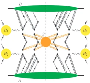
Figure 4. Factorised form of the double Drell-Yan process in the TMD formalism. Double lines denote Wilson lines. The colour indices of adjacent black blobs of the Wilson lines in the soft and collinear factors are equal and summed over. A corresponding form is obtained in collinear factorisation, with hard subgraphs crossing the final-state cut as in figure3.
Wilson line self-interactions must therefore be explicitly excluded from the matrix elements that define soft and collinear factors. In the overall factorisation formula, these self-interactions cancel. For further discussion we refer to sections 13.3.4 and 13.7.2 of [8].
Wilson lines are defined in position space, and the structure of the factorisation formula is simplified by a Fourier transform from transverse momenta in collinear and soft factors to coordinates in transverse configuration space (often referred to as b space). This replaces convolution integrals in transverse momenta by ordi- nary products.
7. Colour structure. The collinear factors have a nontrivial structure in the colour of the four physical parton lines (or more precisely, of the Wilson lines attached to them, see (2.9)). This is different from single hard scattering, where the two parton lines attached to a collinear factor can only couple to an overall colour singlet.
Colour decompositions for double scattering are given in section 2.3 of [1], see [47, 66] for alternative choices and [67] for a simplification in the gluon sector. If the colours of the two partons with the same momentum fraction (x1 orx2) are coupled to singlets, we speak of “colour singlet” double parton distributions, which are an immediate generalisation of the familiar distributions for a single parton. In (2.9) one then contracts j′ with j and k′ with k. Other colour combinations, referred to as “nonsinglet” channels, can be regarded as describing colour interference or colour correlations. In the basis of [1], the second colour structure for two-quark distributions is called “colour octet” combination and obtained by contracting (2.9) withtaj′jtak′k.
JHEP01(2016)076
In TMD factorisation, the hard subgraphs for double Drell-Yan production have a trivial colour structure since their final state is colourless. As a consequence, Wilson lines in the soft factor have their colour indices contracted pairwise, with one Wilson line alongvRand the other alongvL in each pair. Regarding colour indices, the cross section thus involves a matrix multiplication of the form
BT ·S·A=BcScdAd (2.10)
where cand dlabel the different terms in the colour decompositions of A, B and S and are to be summed over. (In the basis just described,canddrun over the singlet and octet channels.)
In collinear factorisation the hard factors can produce unobserved jets, so that sev- eral colour channels are open. Taking qq¯annihilation as an example, one can then decompose
Hjk,j′k′ = 1 Nc
1H δjkδk′j′ + 1 CF
8H tajktak′j′
(2.11) wherej, k are the colour indices of the incoming partons in the amplitude, andj′, k′ those in the conjugate amplitude. The tree-level graph forH contributes only to1H, whereas one-gluon emission contributes only to8H. The colour indices ofH are to be contracted with the colour indices of Wilson lines inS. After a corresponding colour decomposition of S, the colour structure of the cross section involves an additional level of matrix multiplication:
BcScd,fgAdH1fH2g, (2.12)
where f, g label the two colour channels of H1,2. This additional complication was not discussed in [1,47], where only the tree-level expression of H was considered.
8. Soft subtraction in collinear factors. As a consequence of the procedure de- scribed in point 4, the collinear factors require subtractions for regions where gluon lines have momenta that are not collinear but soft. As this has not been elaborated on in [1] we briefly explain it here.
According to point 2, soft gluons inside an unsubtracted collinear factor couple to other soft gluons, to a collinear line, or to the Wilson lines. Taking the right-moving factor for definiteness,Aunsub(vA) thus has a soft subgraphS that connects collinear lines with the Wilson lines. Collinear gluons couple to the Wilson lines as well, and because we have a non-abelian theory, the order of gluon attachments is relevant.
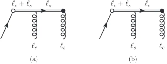
Let us show that a leading contribution is only obtained if, starting at the physical parton line, first all collinear gluons couple to a Wilson line and then all soft gluons, as shown in figure 5a. According to our earlier discussion, vA may have central or large negative rapidity. Since |vAℓc| ≫ |vAℓs| if ℓc is collinear and ℓs is soft, this ordering has the smallest number of eikonal propagators carrying a collinear rather than a soft momentum. Example graphs are shown in figure 6.
JHEP01(2016)076
S
(a)
Asub
S
(b)
Figure 5. (a) The unsubtracted collinear factorAunsub with a soft subgraph that gives a leading contribution. (b) Result of the applying Grammer-Yennie approximations and Ward identities to graph a.
ℓc ℓs
ℓs
ℓc+ℓs
(a)
ℓs ℓc
ℓc
ℓc+ℓs
(b)
Figure 6. The possibilities for one soft and one collinear gluon to couple to a Wilson line. Graph a is leading and graph b is subleading.
One can now apply the same approximations made for soft gluons that couple to the collinear subgraph in the overall process (see point3c), provided that one can again show the cancellation of Glauber gluon exchange. The result has the form
Aunsub(vA) =S(vA, vR)·Asub, (2.13) where by construction the subtracted collinear factorAsubdoes not receive a leading contribution from soft momenta. (It may receive leading contributions from hard loop momenta, but as discussed in point 4 this will be removed by subtractions in the hard factors.) From (2.13) one readily obtains Asub =S−1(vA, vR)·Aunsub(vA).
Note that one can take vA to be lightlike in this expression, since potential rapidity divergences are removed by the soft subtraction term. In the cross section for TMD factorisation one has a product
BsubT ·S(vL, vR)·Asub
=BunsubT (vB)·S−1(vL, vB)·S(vL, vR)·S−1(vA, vR)·Aunsub(vA) (2.14) of matrices in colour space. A corresponding expression is obtained for collinear factorisation from (2.12).
JHEP01(2016)076
For TMD factorisation in single hard scattering, different schemes have been proposed in the literature regarding the choice of Wilson lines. A vectorvA=vB with central rapidity was chosen in [61], whereas vA = vL and vB = vR was taken in [62, 68].
In section 13.7 of [8] a more complicated scheme involving additional soft factors is presented, in which the individual terms in the final factorisation formula do not require the explicit removal of Wilson line self-interactions. vA and vB are taken as lightlike in this scheme. Its analogue for double hard scattering has not been studied so far.
9. Rapidity evolution. In general one cannot take all Wilson lines lightlike, as men- tioned earlier. The collinear and soft factors then depend on the rapidities of the Wilson lines. This dependence is described by differential equations, commonly called Collins-Soper equations. The Collins-Soper equation for the unsubtracted collinear factors has been discussed in section 3.4 of [1]. A derivation of the rapidity evolution for the soft factor in the same framework is still missing. For the particular rapidity regulator introduced within SCET (soft-collinear effective theory) in [64], the rapidity evolution of collinear and soft factors has been discussed in [47].
In collinear factorisation, soft and collinear factors are integrated over transverse parton momenta (or equivalently, evaluated at b = 0 in transverse configuration space). In the colour singlet channel, one can take all Wilson lines as lightlike since potential rapidity divergences cancel. The soft factor then reduces to unity, since it involves Wilson line combinationsW†(v,b=0)W(v,b=0) = 1. In colour nonsinglet channels, one must however keep non-lightlike vectors (or use a different rapidity regulator) and retains nontrivial soft factors.
Factors that depend on a large rapidity difference involve large logarithms, called Su- dakov logarithms (recall that rapidity is a logarithm, see footnote2). The power of these logarithms increases with the order of perturbation theory. The Collins-Soper equations sum these logarithms to all orders and can be used to ensure that the final factorisation formula contains no large logarithms in the hard factors, which can then be evaluated reliably in fixed-order perturbation theory. The resummed Sudakov log- arithms typically lead to a suppression of the cross section. For collinear factorisation this means in particular that all channels except for the colour singlet channel in the double parton distributions are suppressed, as was realised long ago [69]. A simple but instructive numerical study of the suppression of colour nonsinglet channels is given in [47].
10. UV subtractions. Finally, UV subtractions are made in the individual factors as necessary, after which the regulator of UV divergences can be removed (i.e. by taking dto 4 in dimensional regularisation). It is important to do this at the very end, since the rearrangement of soft factors and change of auxiliary vectors discussed in point8 changes the nature of the UV singularities as explained in sections 10.8.2 and 10.11.1 of [8]. Specifically, the limits of taking Wilson line rapidities to infinity anddto 4 do not commute.
JHEP01(2016)076
(a) (b)
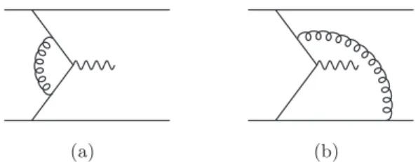
Figure 7. Examples for soft gluon exchange in a simple spectator model. The graphs are under- stood to be embedded in larger graphs for the cross section of single or double Drell-Yan production.
The UV subtractions do not change the overall cross section, where the UV diver- gences in the individual factors cancel, as ensured by the subtraction procedure of point 4. As mentioned earlier, the only UV divergences in the original graphs are those removed by the counterterms in the Lagrangian.
The UV subtracted factors depend on a renormalisation scaleµ. For TMD functions, the dependence on that scale is given by simple renormalisation group equations with anomalous dimensions multiplying the factors themselves. For collinear parton distributions, one obtains DGLAP type equations containing a convolution product of the distributions with splitting functions, where the convolution is in longitudinal momentum fractions. For double parton distributions, these equations are discussed in [70–74]. Their form is connected with the double counting problem noted in point 2c, as explained in section 5.3.2 of [1]. As usual, the evolution equations can be used to ensure that the hard factors do not contain large logarithms that would spoil a fixed-order perturbative expansion.
2.2 Scaling of soft momenta
The typical size of collinear momenta, (ℓ+, ℓ−,|ℓ|) ∼ (Q,Λ2/Q,Λ) or (Λ2/Q, Q,Λ), is directly connected to the external kinematics of the process. Their large components must be of orderQ to enable the hard scattering. Their small and transverse components correspond to generic virtualities of order Λ2 in collinear factorisation, where there is no small external kinematic quantity and Λ is a generic nonperturbative scale. If in TMD factorisation the measured transverse momenta q are larger than a nonperturbative scale, then one must take Λ∼ |q|as discussed earlier. The transverse momenta entering the hard scattering must then be of size Λ in order to produce the required q in the final state.
The size of soft momenta is not directly set by external kinematics. The Libby-Sterman analysis only specifies that all soft momentum components vanish in the formal limit Λ→0.
A crucial part of the analysis is that soft gluons couple to collinear lines.
Let us take a closer look at soft momentum scalings that give a leading contribution to the cross section. For definiteness we consider the exchange of a single soft gluon between the collinear subgraphs A and B, with example graphs given in figure 7. Our discussion applies likewise to single and double Drell-Yan production. Leading regions can be conveniently identified by comparing the expressions for the graph with and without
JHEP01(2016)076
soft gluon exchange:
Z d4ℓ
ℓ2 A(1)++B(1)−− vs. A(0)+B(0)−. (2.15) Here the Lorentz index of the lowest-order expressions A(0) and B(0) originates from the Fierz decomposition mentioned in point3b, and the additional index inA(1)andB(1)comes from the exchanged gluon. The size of each collinear factor can be determined by boosting to a frame where its momenta scale like (Λ,Λ,Λ). In such a frame, all components of A(0) andB(0) scale like Λn(wherenis the appropriate mass dimension), whilst all components ofA(1) and B(1) scale like Λn−1. Boosting back to the overall c.m. frame, we find that the largest components of each factor scale like
A(0)+, B(0)− ∼QΛn−1, A(1)++, B(1)−−∼Q2Λn−3. (2.16) In (2.15) we have already used that other components ofAandBgive smaller contributions and neglected these. A momentum region in the one-gluon exchange graph thus contributes to the cross section with the same power as the leading-order graphs if d4ℓ/ℓ2 ∼ Λ4/Q2, where d4ℓis to be understood as the size of the integration volume for that region.
The preceding analysis is only valid if ℓ+ and ℓ− are at most of order Λ2/Q, so that they do not change the scaling of momenta in the collinear factors. Ifℓ−∼Λ then at least one line inA(1) has momentum scaling like (Q,Λ,Λ) and hence a virtualityQΛ instead of Λ2. A corresponding statement holds for B(1) ifℓ+ ∼Λ. The approximations for collinear momenta discussed in point3 of section2.1 remain valid in this case.
A number of different momentum scalings forℓgive a leading contribution to the cross section.
1. In the Glauber region defined in (2.6) we have ℓ∼ (Λ2/Q,Λ2/Q,Λ), so that d4ℓ∼ Λ6/Q2 andℓ2∼Λ2. Since the collinear factors scale like (2.16) in this case, we obtain a leading contribution.
2. If all components ofℓare of size Λ2/Qthen d4ℓ∼Λ8/Q4 andℓ2∼Λ4/Q2, so that we again obtain a leading contribution. Momenta in this region are often calledultrasoft in the context of effective theories.
Since in this region the typical gluon virtuality goes to zero for Q → ∞, one may wonder whether nonperturbative effects such as confinement invalidate this analysis.
Taking a nonzero gluon mass mg to simulate such effects, one finds that ultrasoft scaling only gives a leading contribution if Λ2/Q&mg.
3. If all components of ℓ are of size Λ, which in effective theories is often denoted as the soft3 region, we have d4ℓ ∼ Λ4 and ℓ2 ∼ Λ2. The scaling in (2.16) must be amended for the presence of collinear lines with virtuality QΛ. One finds that for the graph in figure 7a there is an overall penalty factor (Λ/Q)2 for one off-shell
3Throughout this paper we will use the term “soft” to denote the full region of momenta with components of size Λ or smaller.
JHEP01(2016)076
line in each subgraph A(1) and B(1), so that one obtains a leading contribution. In figure7b the subgraphA(1) has two quark lines with virtualityQΛ, which results in an overall penalty factor (Λ/Q)3 and thus in a power suppressed contribution to the cross section.
4. The regions where ℓ scales like (Λ,Λ2/Q,Λ) or (Λ2/Q,Λ,Λ) may be regarded as hybrids between regions 1 and 3. With d4ℓ∼Λ5/Qandℓ2∼Λ2 and a penalty factor of Λ/Q for an off-shell line in only one of the two collinear factors, these regions contribute to leading power for the appropriate graphs.
This list is not complete, and other scalings such asℓ∼(Λ,Λ2/Q,Λp
Λ/Q) give a leading- power contribution as well. Fortunately, a complete inventory of all leading momentum scalings is not needed for the factorisation proof. In the subtraction procedure sketched in point 4 of section2.1, a regionR is not primarily characterised by its momentum scaling, but by the approximationsTRappropriate for that region. A controlled power-law accuracy of these approximations is an essential ingredient in establishing the method. For a detailed discussion we refer to section 10.7 of [8] and to sections VIII A to D of [61].
For the momentum scalings enumerated above, the Grammer-Yennie approxima- tion (2.5) for a soft gluon coupling to A and its analogue for a soft gluon coupling to B work in regions 2 and 3, but at least one of the approximations fails in regions 1 and 4.
To establish the cancellation of Glauber gluon exchange, we will deform ℓout of regions 1 and 4 into region 2.
2.3 Approximations for soft gluons
As stated earlier, we approximate a soft gluon momentum ℓ entering the collinear factor A(ℓ) by ˜ℓ= (0, ℓ−,ℓ). The Grammer-Yennie approximation
Sµ(ℓ)Aµ(˜ℓ)≈S−(ℓ) vR+
ℓ−vR++iεℓ−A+(˜ℓ)≈Sµ(ℓ) vµR
ℓvR+iε ℓ˜νAν(˜ℓ) (2.17) then fails ifℓ is in the Glauber region.
A different kinematic approximation is described in section 10.4.2 of [8], where ˜ℓ = (0, ℓ−−δ2ℓ+,0), with δ being a parameter of order Λ/Q. (The same approximation with δ = 0 was taken in the original work [50].) The second step of (2.17) is then valid even in the Glauber region. However, the approximation to neglect ℓ inside A(ℓ) is not. The transverse momentum of the soft and collinear lines is comparable not only in the Glauber region but also in regions 3 and 4 described in the previous subsection. In section 3.2 of [50] an argument was given why one can nevertheless neglect ℓ in A for single Drell- Yan production, which required a specific routing of loop momenta. Let us see why this argument does not readily generalise to the double Drell-Yan case.
In figure 8a we show the graphs for a soft gluon coupling to A on the left of the final- state cut in a simple spectator model. After contour deformation out of the Glauber region and use of the Grammer-Yennie approximation, a Ward identity converts the sum of these graphs into collinear factors without a soft gluon, as shown in figure 8b. As in section 3.2
JHEP01(2016)076
k1+ℓ k2
k1+ℓ k2 k1+ℓ k2
k2
k1+ℓ
ℓ ℓ
(a)
k1 k2 k1+ℓ k2−ℓ
ℓ ℓ
(b)
Figure 8. Graphs in a simple spectator model for the part of the collinear factor that is left of the final-state cut (denoted by the dashed line). The incoming line in each graph represents the hadron, which is colourless and thus does not directly couple to gluons. (a) Graphs with one soft gluon coupling to the collinear factor. (b) Result of applying the Grammer-Yennie approximation and a Ward identity.
of [50] we have routed the gluon momentum such that it does not cross the final-state cut.
In order to apply the Ward identity we must use the same external momentum assignment in each graph, and for definiteness we have chosen ℓto flow out of the line with k1 rather than the one with k2. The collinear factor in the first term of figure 8b does not depend on ℓ, so that we obtain the correct result whether or not we set ℓ to zero in the original graphs of figure8a (the eikonal propagators do not depend on ℓand the gluon propagator is to be truncated in all graphs). In the case of single hard scattering, this would be the only term to consider.
The collinear factor in the second term of figure 8b depends however on ℓ, which can be of the same size ask1 and k2, as discussed in the previous subsection. Neglecting ℓin this factor gives an incorrect result. Following the derivation in section 3.2.2 of [1] one finds indeed that in the overall expression of the cross section, the dependence of this collinear factor on ℓ is crucial to give the correct transverse position of the Wilson lines to which the soft factor is eventually converted. This holds true even for collinear factorisation, where the Wilson lines associated with the partons of momentak1 and k2 have a relative transverse distance y from each other. Neglecting ℓ in the graphs of figure 8a would put all Wilson lines in the soft factor at the same transverse position, which is incorrect.
JHEP01(2016)076
3 Glauber cancellation for one-gluon exchange
3.1 Scope and general method
In this section we demonstrate the cancellation of Glauber gluons in the double Drell-Yan process at the level of single gluon exchange. The momentum ℓ of the exchanged gluon can lie in the hard, soft, or collinear-to-A or B regions, and what we shall show in this section is that the approximated expressions from these regions reproduce the exact graph at leading-power accuracy. There is no need for a separate term for the Glauber region, where the soft Grammer-Yennie approximation (2.5) breaks down. The hard region can be distinguished from the rest by the fact that it corresponds to generically large transverse momenta |ℓ| ∼ Q rather than |ℓ| ∼ Λ. By considering integrals differential in transverse momenta, and transverse momenta only of order Λ, we remove the need to consider the hard region in the following.
For simplicity, we adopt a model with scalar “partons” described by a field φ and coupling to each other via three- and four-point vertices. Gluons couple to these partons as required by gauge invariance, i.e. via the usual scalar QED/QCD-type vertices (see for example [75]). We thus have a momentum-dependentgφφvertex and aggφφseagull vertex.
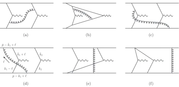
Some example graphs for the double Drell-Yan process in this model are given in figure9.
We shall not concern ourselves with the detailed colour structure of the model. As we shall see, the Glauber cancellation argument depends only on the analyticity properties of the loop integrands in the gluon momentum, which in turn is determined only by the denominators of the Feynman and eikonal propagators. It does not rely on the spin and colour structure of the model, and hence also applies to graphs in QCD.
The Glauber cancellation argument we shall present here works on a graph-by-graph basis, with the sum over cuts of the graph taken where necessary. We need to consider only graphs in which the gluon extends between right- and left-moving collinear partons — graphs in which the gluon attaches only to right- or left-moving partons are topologically factorised already. We classify the partons into active ones and spectators, with active partons being the ones that attach to a vertex producing an electroweak gauge boson. All other partons are spectators. We thus have active-active, active-spectator, and spectator- spectator gluon attachments.
What we shall do in this section corresponds to applying the region approximants of point 3 in section 2.1 in the following order: first we make contour deformations needed to avoid the Glauber region (with a sum over cuts where necessary). Then we apply the Grammer-Yennie approximations, before deforming the contours back to the real axis.
Finally the kinematic approximations and approximations for fermion lines are applied.
With this order of steps, we do not need to concern ourselves with the kinematical and fermion line approximations in this section.
To illustrate where problematic pinched poles in ℓ+ or ℓ− may generically arise, it is instructive to consider the example graph in figure9d. Ifℓis in the Glauber region thenℓ− is negligible in the right-moving lines above the gauge boson vertices. It is also negligible in gluon propagator, which is dominated by ℓ2. Poles in the small ℓ− region thus result