Power corrections and renormalons in Transverse Momentum Distributions

JHEP03(2017)002

Published for SISSA by Springer

Received: September 26, 2016 Revised: January 16, 2017 Accepted: February 15, 2017 Published: March 1, 2017

Power corrections and renormalons in Transverse Momentum Distributions

Ignazio Scimemi

and Alexey Vladimirov

aDepartamento de F´ısica Te´orica II, Universidad Complutense de Madrid, Ciudad Universitaria, 28040 Madrid, Spain

bInstitut f¨ur Theoretische Physik, Universit¨at Regensburg, D-93040 Regensburg, Germany

E-mail: ignazios@fis.ucm.es, aleksey.vladimirov@gmail.com

Abstract: We study the power corrections to Transverse Momentum Distributions (TMDs) by analyzing renormalon divergences of the perturbative series. The renormalon divergences arise independently in two constituents of TMDs: the rapidity evolution ker- nel and the small-b matching coefficient. The renormalon contributions (and consequently power corrections and non-perturbative corrections to the related cross sections) have a non-trivial dependence on the Bjorken variable and the transverse distance. We discuss the consistency requirements for power corrections for TMDs and suggest inputs for the TMD phenomenology in accordance with this study. Both unpolarized quark TMD parton distribution function and fragmentation function are considered.

Keywords: Effective field theories, Perturbative QCD, Renormalization Regularization and Renormalons, Resummation

ArXiv ePrint: 1609.06047

JHEP03(2017)002

Contents

1 Introduction 1

2 Notation and basic concepts 3

3 TMD in large-β

approximation and renormalon divergences 6

3.1 The soft function in the large-β

approximation 6

3.2 The TMD in the large-β

approximation 8

3.3 The TMD anomalous dimensions at large-β

and renormalon singularities

of D 9

3.4 TMD matching coefficient at large-β

11

3.5 Lessons from large-β

12

4 Renormalon substraction and power corrections 13 4.1 Non-perturbative corrections to the anomalous dimension D 14

4.2 Renormalon consistent ansatz for TMDs 17

5 Conclusion 21

1 Introduction

The transverse momentum dependent (TMD) distributions are fundamental non- perturbative objects that appear in many relevant processes at LHC, EIC, and e

e

colliders, like Vector Boson Production, Higgs production, Semi-Inclusive Deep Inelastic Scattering, e

e

→ 2 hadrons. The factorization theorems which establish the definitions of TMD distributions in QCD and/or in effective field theory have been formulated recently in [1–4], using different regularization schemes.

The perturbative properties of unpolarized TMDs, such as evolution and operator product expansion (OPE) in the regime of small transverse momentum separation, have been deduced by several groups using different frameworks (see e.g. [1, 2, 4–9]). The explicit direct calculation of the TMD evolution function D at NNLO has been provided in [10, 11]

and recently it was obtained at N

LO [12]. Therefore, nowadays the perturbative knowledge of the unpolarized TMDs parton distribution functions (PDFs) and fragmentation functions (FFs) is comprehensive, thanks to the results obtained by various groups [11, 13–19].

On the contrary, the study of the non-perturbative properties of TMDs has been based mainly on phenomenological arguments which combine the perturbative information on TMDs with their perturbatively incalculable part [4, 8, 20–25]. These works have lead to different forms of implementation of TMDs which in general are not easy to compare.

For instance, on one hand, the well-known phenomenological considerations of Drell-Yan

JHEP03(2017)002

by [26] and [27] (the so-called BLNY model) implement an ansatz within the standard CSS approach with b

-prescription in the impact parameter space (or b-space). They introduce a set of non-perturbative parameters g

and all these parameters (including the definition of b

prescription) are fundamental for these fits. The same model is also the core of the RESBOS program package [28] which is widely used in applications. On another hand, the implementation of TMDPDFs by [29] does not use b

-prescription. They have found that part of the non-perturbative corrections (essentially to the TMD evolution kernel) are negligible. They were able to describe the same data with a different shape of non-perturbative input parameterized by two parameters λ

. Fits by other groups that limited themselves to the analysis of Vector Boson Production and Higgs production are less sensitive to the non-perturbative input (although it is still necessary) [30, 31].

Additional problems arise in the consideration of TMDFFs which are known to have very different and/or incomparable (in comparison to TMDPDFs) non-perturbative input.

This work is devoted to the study of the leading power corrections to TMD distribu- tions. With this aim, we perform an analysis of the leading renormalon structure of TMD distributions. A renormalon analysis of the perturbative series gives an important check of theoretical consistency for any phenomenological ansatz, although it cannot give too stringent restrictions on the fitting parameters. The study of renormalon poles allows to understand the asymptotic behavior of the perturbative series and to deduce the form of the leading non-perturbative corrections [32–35].

An explicit analysis of the renormalon structure for TMDs has never been done to our best knowledge, although assumptions on its structure were used even before the actual field-theoretical definition of TMDs. We refer here, for instance, to the seminal work of [33]

about the Sudakov factor in differential cross-section which is usually referred to justify a Gaussian behavior for the non-perturbative part of the TMD evolution kernel [25]. In order to describe this effect in the modern TMD framework, we recall that the definition of TMDs requires the combination of the Soft Function matrix element with the transverse momentum dependent collinear function. As we show in this work, the renormalon diver- gences arise in the perturbative consideration of both of these functions. These renormalon contributions have different physical meaning and should be treated independently. Firstly, the renormalon divergence of the soft factor results to a power correction within the TMD evolution kernel, which are strictly universal for any TMD due to the universality of the soft factor itself. The leading power correction that we derive here is quadratic. The presence of these corrections has been shown in [36] by the analysis of the corrections to conformal anomaly. Secondly, the renormalon divergences naturally arise within the coefficients of the small-b OPE. A study of those contributions gives access to the next twist corrections of small-b matching and specifies the shape and the general scaling of TMD.

The paper is built as the following. We provide the necessary concepts and definitions in section 2. In section 3 we perform the calculation of various TMD constituents (such as anomalous dimensions and coefficient functions) within the large-β

approximation.

In the end of this section we provide a collection of the main lessons, that follows from

our results. The impact of the renormalon divergences on the perturbative series and

renormalon subtracted series are studied in section 4. One of the main outcomes of the

study, namely a consistent ansatz for TMDs is presented in section (4.2).

JHEP03(2017)002

2 Notation and basic concepts

Throughout the paper we follow the notation for TMDs and corresponding functions in- troduced in [14]. The quark TMDPDFs and TMDFFs are given by the following matrix elements

F

(x, b; ζ, µ) = Z

(ζ, µ)R

(ζ, µ) 2

× X

X

Z dξ

2π e

hN |

T h

¯ q

W ˜

i

a

ξ 2

|Xiγ

hX| T ¯ h

W ˜

q

i

a

− ξ 2

|N i,

∆

(z, b) = Z

(ζ, µ)R

(ζ, µ)

4zN

(2.1)

× X

X

Z dξ

2π e

h0|T h

W ˜

q

i

a

ξ 2

|X, N iγ

hX, N | T ¯ h

¯ q

W ˜

i

a

− ξ 2

|0i,

where R

and Z

are rapidity and ultraviolet renormalization constants, q are quark fields and W

are Wilson lines, and ξ = {0

, ξ

, b}. The TMDs depend on the Bjorken variables (x for TMDPDFs and z for TMDFFs), the impact parameter b and the factorization scales ζ and µ. The considerations of the TMDPDF and TMDFF are similar in many aspects.

Therefore, in order to keep the description transparent we mostly concentrate on the case of the TMDPDFs, while the results for TMDFFs are presented without derivation.

The dependence on the factorization scales is given by the evolution equations, which are the same for TMDPDF and TMDFF, namely

d

dlnµ

F

(x, b; ζ, µ) = γ

(µ, ζ)

2 F

(x, b; ζ, µ), (2.2) d

dlnζ F

(x, b; ζ, µ) = −D

(µ, b)F

(x, b; ζ, µ). (2.3) Through the article we consider only the quark TMDs, therefore in the following we sup- press the subscript q on the anomalous dimensions. The values for both anomalous dimen- sions can be deduced from the renormalization constants [14]. Also γ and D are related to each other by the cross-derivatives

dD(µ, b

) dlnµ

= − 1

2

dγ(µ, ζ)

dlnζ = Γ

2 , (2.4)

where Γ

is the honored cusp anomalous dimension.

The solution of the evolution equations eqs. (2.2), (2.3) is

F (x, b; ζ

, µ

) = R(b; ζ

, µ

, ζ

, µ

)F(x, b; ζ

, µ

), (2.5) where R is the evolution kernel,

R(b; ζ

, µ

, ζ

, µ

) = exp Z

µi

dµ µ γ

α

(µ), ln ζ

µ

ζ

ζ

. (2.6)

The final values of scaling parameters is dictated by the kinematic of the TMD cross-

section. The variable ζ

∼ Q

(with Q being a typical hard scale) is the scale of the

JHEP03(2017)002

rapidity factorization, and the variable µ

is the scale of hard subprocess factorization. The intriguing point is that the evolution kernel R is not entirely perturbative, but contains a non-perturbative part. An estimate of the non-perturbative contribution to R is necessary in order to obtain the cross section in the momentum space where it is usually measured.

The non-perturbative part of the evolution kernel is encoded in the D-function which can be obtained from the rapidity renormalization constant R

. The definition of the rapidity renormalization constant differs from scheme to scheme. In this work we use the δ-regularization scheme defined in [10, 14]. In this scheme, the δ-regularization is used to regularize the rapidity divergences, and the dimensional regularization regularizes the rest of divergences. Such a configuration appears to be very effective for the TMD calculus.

In particularly, the rapidity renormalization factor R

is expressed via the soft factor S as R

= S

[14]. In the coordinate space the soft factor is given by the following matrix element

S(b ˜

) = Tr

N

h0| T h

S

S ˜

i

(0

, 0

, b) ¯ T

h S ˜

S

i

(0) |0i , (2.7)

where we explicitly denote the ordering of operators and S

are Wilson lines, as defined in [10]. Considering the relation between renormalization constants one can show [10], that

D = 1 2

dln ˜ S dl

(2.8) where l

= ln(µ

/|δδδ|). Eq. (2.8) can be used as the formal definition of the TMD evolution function D. In this way, a non-perturbative calculation of the SF gives access to the non-perturbative structure of D. The soft function is perturbatively universal for both Semi Inclusive Deep Inelastic Scattering and Drell-Yan type processes. Therefore, the perturbative part of the anomalous dimension D is universal for TMDPDF and TMDFF.

One can also expect its universality in the non-perturbative regime.

The TMDs are entirely non-perturbative functions. They cannot be evaluated in per- turbative QCD, due to the non-perturbative origin of hadron states. The main subject of the paper is the dependence of TMDs on the parameter b which is generically unrestricted since it is a variable of Fourier transformation. However it is interesting and numerically important to consider the range of small b (here and later b = √

b

). In this range, the TMDs can be matched onto corresponding integrated parton distributions. At the operator level, the small-b matching is given by the leading term of the small-b OPE. The small-b OPE is a formal operator relation, that relates operators with both light-like and space-like field separation to operators with only light-like field separation. It reads

O(b) = X

n

C

(b, µ

) ⊗ O

(µ

), (2.9)

where C

are Wilson coefficient functions, the µ

is the scale of small-b singularities fac-

torization or the OPE matching scale (for simplicity we omit in eq. (2.9) other matching

scales included in the definitions of each component of this equation). Generally, the oper-

ators O

are all possible operators with proper quantum numbers and can be organized for

JHEP03(2017)002

instance according to a power expansion, i.e. twists. In this case, the matching coefficients behave as

C

(b, µ

) ∼ b

B

f (ln(b

µ

)), (2.10)

where f is some function. The value of the parameter B is unknown, and its origin is entirely non-perturbative. In other words, the unknown scale B represents some charac- teristic transverse size of interactions inside a hadron B ' O(1 GeV). In practice it is reasonable to consider only the leading term (n = 0) of eq. (2.9) for b B. In this case, f is an integrated parton distribution (or fragmentation function), and coefficient function is called the matching coefficient. So far, the power suppressed terms in eq. (2.9) has been not considered, to our best knowledge.

For completeness, we recall here the renormalization group properties of the TMD Wilson coefficients that we use in the following sections. The evolution equations for the matching coefficients (at µ

= µ) with respect to ζ is

d

dlnζ C

(x, b

; µ, ζ ) = −D

(µ, b

)C

(x, b

; µ, ζ ), (2.11) where f = q, g species, C

are the matching coefficients on PDFs. It is practically convenient to extract the ζ-dependence from the matching coefficient. We introduce the notation

C

(x, b

; µ, ζ ) = exp

−D

(µ, b

)L

C ˆ

(x, L

). (2.12) Here and further we use the following notation for logarithms

L

= ln

X

b

4e

, l

= ln µ

X

. (2.13)

The ζ-free coefficient function ˆ C satisfies the following renormalization group equation µ

d

dµ

C ˆ

(x, L

) = X

r

Z

dy y C ˆ

x y , L

K

(y, L

), (2.14) where the kernel K is

K

(x, L

) = δ

δ(1 − x) 2

Γ

L

− γ

− P

(x),

and P(x) is the splitting function (DGLAP kernel). The matching coefficient for TMDFF

C

satisfies the same set of evolution equation with only substitution of PDF splitting

function P (x) by the FF ones, P (z)/z

[14]. Using these equations one can find the expres-

sion for the logarithmic part of the matching coefficients at any given order, in terms of the

anomalous dimensions and the finite part of the coefficient functions. The expressions for

the anomalous dimensions, the recursive solution of the RGEs and the explicit expressions

for the coefficients C and C can be found, e.g. in [14].

JHEP03(2017)002

3 TMD in large-β

approximation and renormalon divergences

The leading non-perturbative contribution to the perturbative series is commonly associ- ated with renormalons. The renormalon contributions were intensively studied for various matrix elements and in different regimes, for review see [37, 38]. A typical signature of renormalons is the factorial divergence of the perturbative series. These divergences are often discussed in terms of the corresponding singularities in the Borel plane.

The best representative and the only stable way to study the renormalon divergence within perturbative QCD is the large-β

approximation. The large-β

expression can be obtained from the large-N

expression through the procedure of “naive Abelianiza- tion” [39, 40]. In this section, we present the calculation of large-β

correction to TMDs.

Since the technique of large-N

calculus is well-known, we skip the detailed evaluation (redirecting the reader to the related literature) and present only intermediate expressions.

3.1 The soft function in the large-β

approximation

The soft function matrix elements is a key structure for the TMD construction and as such it is a good starting point for the renormalon analysis. The large-β

calculation of the soft factor runs in parallel to the calculation of the integrated soft factor for Drell-Yan, which is presented in [32] (see section 5.3). Here we present our results of the evaluation.

To begin with, we evaluate the large-N

contribution to the soft factor, which is given by the “bubble” resummed diagram, shown in figure 1.A. The expression for the (renor- malized) diagram with n-bubble insertion is

SF

= − 4C

β

a

β

−

!

X

k=0

n!

k!(n − k)! (3.1)

(−1)

n − k + 1 G(−, −(n + 1 − k)) (L

− ψ(−(n − k + 1)) − γ

) ,

where β

=

T

N

, a

= g

/(4π)

, is the parameter of dimension regularization (d = 4 − 2), δδδ = |2δ

δ

| with δ

the being parameters of rapidity regularization for Wilson lines pointing in n(¯ n)-direction [14]. The function G is a standard function that appears in the large-β

calculation [32, 37, 39, 40], and is given by the expression

G(, s) = e

B B B

A

Γ(1 + s)

Γ(1 − s + ) , (3.2)

with

A

= 6Γ(1 + )Γ

(2 − )

Γ(4 − 2) , B B B

= b

µ

4e

.

Here, the Euler-Mascheroni constant is a result of the MS scheme. For n = 1, 2 this expression agrees with the direct calculation of the soft factor in δ-regularization [10]. We also introduce an additional function for the double-pole part

G(, s) = ˜ −G(, s)(ψ(s) + γ

). (3.3)

JHEP03(2017)002

Figure 1. Diagrams contributing to the leading order of large-Nf limit. The diagram A is the contribution to the soft factor. Diagrams B and C are contribution to the matching coefficient.

The counter term diagrams are not shown.

The functions G and ˜ G have the following Taylor series G(, s) =

∞

X

j=0

G

()s

=

∞

X

j=0

s

∞

X

k=0

g

, (3.4)

G(, s) = ˜

∞

X

j=0

G ˜

()s

=

∞

X

j=0

s

∞

X

k=0

˜

g

. (3.5) These expressions define the coefficients g

and G

. Note, that g

= ˜ g

and g

= ˜ g

.

The procedure of “naive Abelianization” consists in the replacement of N

by the corresponding β

expression [39], i.e.

β

= 4

3 T

N

−→ −β

= − 11

3 C

+ 4

3 T

N

. (3.6) In this way, we obtain the large-β

expression for the soft factor

SF = −

∞

X

n=0

4C

c

β

"

(−1)

n!

L

G

(−) + ˜ G

(−)

(3.7) + (−1)

n + 1 −L

G

(−)

+

G ˜

(−)

(ψ(n + 2) + γ

) − G ˜

(−)

! # ,

where we have introduced the large-β

coupling constant c

= β

a

> 0.

Note, that in eq. (3.7) the terms suppressed in are dropped.

Eq. (3.7) gives access to the anomalous dimension D, which we study in section 3.3, and to the rapidity renormalization factor R

. The factor R

(we recall that it is equal to R

= S

in the δ-regularization [14]) from the perspective of the large-β

approximation has the same perturbative combinatorics as the one-loop-truncated pertrubation series. It is given by

R

= 1 − SF

2 (3.8)

at δ

= ζ/p

and SF given in eq. (3.7). This expression is used in the next section to

extract the large-β

expression of the Wilson coefficients of small-b OPE.

JHEP03(2017)002

3.2 The TMD in the large-β

approximation

To obtain the TMD matching coefficient one should evaluate the diagrams B and C, which are shown in figure 1. The result for the sum of these diagrams and their Hermitian conjugations is

Φ

= 2C

β

∞

X

n=0

(a

β

)

(−)

n

X

k=0

n!

k!(n − k)!

(−1)

G(−, −(n − k + 1))

n − k + 1 (3.9)

"

¯

xx

(1 − )(1 + (n − k)) + 2 x

(1 − x)

− 2δ(¯ x)ln δ

p

#

,

where we have used the same notation as in eq. (3.1) and ¯ x = 1 − x. The last term in square brackets represents the rapidity divergence which appears in the diagram C. For n = 0, 1 this expression reproduces the result of explicit calculation made in [13].

Using eq. (3.8) and eq. (3.9) we can complete the result for the large-N

expression of the TMDPDF,

R

Φ = Φ

− SF

2 = 2C

β

∞

X

n=0

(a

β

)

(−)

n

X

k=0

n!

k!(n − k)!

(−1)

G(−, −(n − k + 1))

n − k + 1 (3.10)

"

¯

xx

(1−)(1+(n−k)) + 2 x

(1 − x)

+ δ(¯ x) (L

−l

−ψ(−(n−k+1)) − γ

)

# . Here, we observe the cancellation of the rapidity divergences that leaves the residual l

dependence.

In order to extract the matching coefficient of the TMDPDF onto the PDF one has to proceed to the renormalization of eq. (3.10). This is greatly simplified in the δ- regularization scheme, where all virtual graphs and integrated graphs are zero. The only non-zero contribution is the UV counterterm which is a pure -singularity. The accounting of this part eliminates terms singular in , leaving the finite part unchanged. The latter provides the coefficient function. Performing the “naive Abelianization” as in eq. (3.6) we obtain the large-β

result

C

= 2C

β

∞

X

n=0

c

("

¯

x + 2 x (1 − x)

#"

γ

(x)

n + 1 + (−1)

n!g

[B B B

]

#

(3.11) + x ¯

n + 1 (2γ

(x) + γ

(x)) − x(−1) ¯

n!g

[B B B

] +δ(¯ x) (L

− l

)

"

g

n + 1 + (−1)

n!g

#

+δ(¯ x)

"

˜

g

ψ(n + 2) + γ

n + 1 + ˜ g

(n + 1) + (−1)

n!˜ g

#) ,

where B B B

= xB B B

, and

x

G

() =

∞

X

k=0

γ

.

JHEP03(2017)002

The additional variable in the square brackets for the functions g indicates the modified value of B B B

to be substituted.

The calculation of TMDFFs matching coefficient proceeds in the same way as for TMDPDFs. The result of the calculation is

z

C

= 2C

β

∞

X

n=0

c

("

¯

z + 2 z (1 − z)

#"

γ

(z

)

n + 1 + (−1)

n!g

[B B B

]

#

(3.12) + z ¯

n + 1 2γ

(z

) + γ

(z

)

− z(−1) ¯

n!g

[B B B

] +δ(¯ z) (L

− l

)

"

g

n + 1 + (−1)

n!g

#

+δ(¯ z)

"

˜

g

ψ(n + 2) + γ

n + 1 + ˜ g

(n + 1) + (−1)

n!˜ g

#

−

n+1

X

r=1

¯ z + 2z

1 − z

γ

(z) + ¯ z(2γ

(z) + γ

(z)

(−1)

ln

(z

) (n + 1)r!

) . One can see that the expression for TMDPDF eq. (3.11) is related to the first four lines of the expression for TMDFF eq. (3.12) by the crossing relation x → z

. The last line of eq. (3.12) is specific for TMDFF and it is an effect of the expansion of the normalization factor z

.

One can check that at n = 0, 1 the expressions (3.11) and (3.12) coincide with the one calculated in [14].

3.3 The TMD anomalous dimensions at large-β

and renormalon singularities of D

In the articles [10, 14] it was shown that in the δ-regularization scheme the anomalous dimension D can be obtained from the rapidity singular part of the soft factor as in (2.8).

Considering the eq. (3.7) we obtain the anomalous dimension D in the large-β

approxi- mation

D = − 2C

β

∞

X

n=0

c

(−1)

n!g

+ g

n + 1

!

. (3.13)

The first term in the brackets of eq. (3.13) behaves ∼ n! at large n, and represents the renormalon singularity.

At this point it is convenient to consider the Borel transformation of the result. We define the Borel transformation of a perturbative series in the usual way

f(c

) =

∞

X

n=0

f

c

= ⇒ B[f ](u) =

∞

X

n=0

f

u

n! . (3.14)

A perturbative series is Borel summable if an integral f ˜ =

Z

due

B[f ](u), (3.15)

JHEP03(2017)002

exists. Performing the Borel transformation on the D function and applying eq. (3.15), we find

D = − 2C

β

Z

0

dx G(x, 0) − 1

x −

Z

du G(0, −u) − 1 u e

. (3.16)

The first term is analytical and reproduces the cusp-anomalous dimension at large-β

[32]

Γ

(c

) = 4C

c

β

Γ(4 + 2c

)

6Γ

(2 + c

)Γ(1 + c

)Γ(1 − c

) = 4C

c

β

G(c

, 0). (3.17) The function which appears in the second term

G(0, −u) = B B B

e

Γ(1 − u)

Γ(1 + u) , (3.18)

contains a series of poles at u = 1, 2, . . . which correspond to infrared renormalons. One can check explicitly that the relation eq. (2.4) holds for large-β

expression, due to cancellation of the renormalon divergences in the second term of eq. (3.16) between derivative of coupling constant (in the Borel exponent) and derivative of B B B

(in the function G(0, −u)).

There are multiple possibilities to define the sum eq. (3.13), e.g. one can slightly shift the integration contour for eq. (3.16) into the complex plane. The difference between integrals passing from the lower and upper sides of poles is called infrared (IR)-ambiguity and is given by a (−π) times the residue at the pole. For the anomalous dimension D it reads

δ

{D} = cb

Λ

, (3.19)

where

c = πC

2β

e

' 1.2. (3.20)

The IR-ambiguity represents the typical scale of the error for perturbative series.

The same conclusion, namely the presence of a b

-correction for D, was made in ref. [36]

using different argumentation. In ref. [36] the factorized cross-section has been considered within the soft collinear effective field theory (SCET). It has been shown that the power correction to the soft factor which arises in the next-to-leading term of large-Q

OPE, is proportional to the soft factor matrix element. Exponentiating the power correction one obtains the same result as presented here. It is an expected agreement because the renormalon calculation is equivalent to the calculation of the correction term of OPE.

The anomalous dimension γ

can be extracted from the coefficient function eq. (3.11).

We consider the derivative of coefficient function at l

= L

µ

d

dµ

C ˆ

(x, L

) = Z

x

dy y C ˆ

x y , L

1

2 (Γ

L

− γ

) δ(¯ y) − P

(y)

, (3.21) where we have dropped the mixing among flavors. The DGLAP kernel at large-β

is given by the expression

P

(x) = 2C

β

∞

X

n=0

c

( 1 + x

1 − x γ

(x) + ¯ x(2γ

(x) + γ

(x)) )

+

. (3.22)

JHEP03(2017)002

Considering the derivative of eq. (3.11) and comparing right and left hand sides of eq. (3.21) we obtain

γ

= − 4C

β

( c

ψ(1 + c

) + 2γ

+ 3 − c

(1 + c

)(2 + c

)

G(c

, 0) (3.23) +ln (G(c

, 0)Γ(1 + c

)) G(c

, 0) +

Z

G(xc

, 0) − G(c

, 0)

1 − x dx

) .

This expression contains no singularity, and hence it is renormalon-free, as it is usually expected for an ultraviolet anomalous dimension.

3.4 TMD matching coefficient at large-β

Before the evaluation of the sums in eqs. (3.11)–(3.12) we extract the part related to the anomalous dimension D to obtain the coefficients ˆ C defined in eq. (2.12). This procedure is important since the function D contains its own renormalon singularities, as described in eq. (3.19). The contribution of D is easily recognized in the third lines of (3.11)–(3.12) (compare with eq. (3.13)).

The result of the Borel transform for the coefficient ˆ C, eq. (3.11) is C ˆ = 2C

β

Z

0

due

(

¯

x + 2x (1 − x)

γ γ γ(u) − 1 u + ¯ x

Z

dy(2 + u y)γ ¯ γ γ(yu) +δ(¯ x)

G G G

(u) − 1

u +

Z

dy G G G

(u) − G G G

(yu) u(1 − y)

+

¯

x + 2x (1 − x)

1 − G[B B B

](0, −u) u

− xG[ ¯ B B B

](0, −u) +δ(¯ x) G(0, −u)(ψ(−u) + γ

)

u − 1

u

− L L L

+

u

! )

, (3.24)

where by bold font we denote the Borel transformed functions, G

(u) =

∞

X

n=0

g

u

n! , G G G

(x) = d

dx G G G

(x), γ

(u) =

∞

X

n=0

γ

(x) u

n! . (3.25) The terms in eq. (3.24) are collected such that every bracket is finite at u → 0. The expres- sion for TMDFF coefficient function ˆ C can be obtained using the crossing transformation (x → z

) and the addition of the normalization contribution (the last line in eq. (3.12)).

In the last two lines of eq. (3.24) we have the infrared renormalon poles in u = 1, 2, . . ..

One can see that the third line contains only first order poles, while the last line contains second order poles at G(0, −u)ψ(−u). Considering the infrared ambiguity at u = 1 we obtain

δ

{ C} ˆ = −c(xb

Λ

) (

2¯ x + 2x

(1 − x)

− δ(¯ x)

L

+ 2 3

)

, (3.26)

JHEP03(2017)002

where constant c is given in eq. (3.20). The x−dependence of this expression exactly reproduces the x−dependence of the leading terms of the next power correction in small-b OPE, see detailed description in [41]. The consideration of ambiguites of higher renormalon poles gives access to the higher-power corrections. We obtain

δ

{ C} ˆ = πC

β

−xb

Λ

e

n!n!

2x (1 − x)

+ (n + 1)¯ x − δ(¯ x)

L

− ψ

− γ

+ 5 3

. (3.27) However, these expressions can be modified by the infrared renormalon contributions of the higher-twist terms. The most important information of the higher-power corrections is that the renormalons scale as xb

, but not as b

which is a naive assumption. The consequences of this fact are discussed in the next sessions.

The corresponding calculation for TMDFF gives δ

{z

C ˆ } = −c

b

Λ

z

(

2¯ z + 2z (1 − z)

− δ(¯ z)

L

+ 2 3

)

. (3.28)

which is the same as eq. (3.26) with the crossing change x → 1/z. One can see that the difference in normalization which spoils the crossing between TMDPDFs and TMDFFs, disappears in the renormalon contribution. The higher poles ambiguites are provided using the crossing relation x → 1/z in eq. (3.27).

3.5 Lessons from large-β

The eqs. (3.19), (3.26), (3.28) are one of the main results of this work. These expressions represent the leading power correction to the small-b regime, where all perturbative prop- erties of TMDs are derived. These expressions give access to a general structure of the next-to-small-b regime. The practical implementation of results eqs. (3.19), (3.26), (3.28) is given in the next section, while here we collect the most important observation that follows from the large-β

calculation and which should be taken into account for TMD phenomenology.

The first, and the most obvious, observation is that the leading power corrections are

∼ b

. It implies that an exponential decay of the TMDs that is sometimes suggested in phenomenological studies (e.g. [42, 43]) can in no way affect the small-b region. Indeed, it would imply the corrections ∼ √

b

to the small-b OPE, that cannot appear without extra scaling parameter. Nonetheless, exponential corrections can occur in the large-b regime, which is inaccessible by perturbative considerations.

Second, one can see that the renormalon corrections to TMDPDFs matching coef-

ficient scales like xb

, and not as simply b

(as it is usually assumed), nor as x

b

(as

suggested by Laguerre polynomial decomposition [9]). Therefore, the contributions of

higher-twist terms in small-b OPE for TMDPDF are largely functions of xb

. Correspond-

ingly, TMDFFs matching coefficients are a function of b

/z. This is important in respect

of the phenomenological implementation of the TMDs. For instance, the b

-prescription

JHEP03(2017)002

which is often adopted does not respect this scaling and so, in this sense, it is not fully consistent with the estimated higher twist effects.

Third, the renormalon contributions to the anomalous dimension D and to matching coefficients have different physical origins and do not mix with each other. In fact, the anomalous dimension D is an universal object that is the same for all regimes of b and for TMDs of different quantum numbers [25]. Thus, the renormalon contribution to D rep- resents a generic universal non-perturbative contribution, alike in the case of heavy quark masses. On the other hand, the (infrared) renormalon divergences within the matching co- efficients are to be canceled by the corresponding (ultraviolet) renormalon contributions of higher twists. Therefore, while eq. (3.19) represents a size of a universal non-perturbative contribution, eqs. (3.26), (3.28) give the form of the twist-four contribution to small-b OPE.

In other words, eqs. (3.26), (3.28) estimate very accurately the x-behavior of subleading correction to small-b OPE.

The consideration of the anomalous dimension D for gluon distributions is identical to those of quarks (apart of trivial replacing of the common factor C

by C

). Contrary, the calculation of the renormalon contribution for gluon and quark-gluon matching coefficient is much more complicated than the one presented here and is beyond the scope of this paper. In general, we can expect a non-trivial dependence of the renormalon contribution on the Bjorken variables. At present, we cannot find arguments which suggest a location for the renormalon poles and an xb

scaling different from that of quarks.

4 Renormalon substraction and power corrections

Our analysis is limited to the quark TMDs only. Nonetheless, we can advance some con- siderations on possible inputs, which are consistent with our findings and evaluate their impact on the non-perturbative structure of TMDs. The suggested ansatz for TMDs does not pretend to be unique and moreover is inspired by other popular models. We postpone to a future publication a more dedicated study on the subject.

We recall here the form of the TMDPDFs which emerges at small-b is F

(x, b; ζ

, µ

) = R(b, ζ

, µ

; ζ

, µ) X

j

Z

dy y

C ˆ

x y , b; µ

f

(y, µ), (4.1) where the evolution kernel R is given in eq. (2.6). The argument ζ

of R is collected from the combination of two exponents: the original factor R (2.6) and the exponential prefactor of ˆ C (2.12), and it takes the value

ζ

= 4e

b

.

The analogue equation for TMDFFs is obtained replacing consistently the PDF f

by

the fragmentation function d

and the coefficient function C

by C

, while the

evolution kernel remains the same. This expression is usually taken as an initial ansatz for

TMD phenomenology.

JHEP03(2017)002

As we pointed earlier there are two places where the non-perturbative effects arise. The first one is the evolution kernel D which is a part of the evolution prefactor R, and it is common for all TMDs (TMDPDFs and TMDFFs of various polarizations). The second one is the higher twist corrections to the small-b OPE. These non-perturbative contributions are of essentially different origin and should not be mixed. In particular it is important to realize that the non-perturbative contribution of D enters eq. (4.1) as a prefactor, while the higher order terms of OPE are added to the convolution integral. Therefore, the structure of non-perturbative corrections to TMD that we keep in mind is the following

F

(x, b; ζ

, µ

) = exp ( Z

µ

dµ

µ

γ µ

, ζ

)

ζ

ζ

× (4.2)



 X

j

Z

dy y

C ˆ

x y , b; µ

f

(y, µ) + f

(x, b; µ)



 .

Here, D

is the non-perturbative addition to the anomalous dimension D, and f

is the cumulative effect of the higher twist corrections to the small-b OPE. At small (perturbative) b, the non-perturbative parts should turn to zero, such that eq. (4.2) reproduces eq. (4.1).

In the following subsections we construct a minimal non-contradicting anzatz for TMD distributions that respect the study of large-β

approximation.

4.1 Non-perturbative corrections to the anomalous dimension D

The non-perturbative part of the anomalous dimension D is one of the most studied in the literature and the one for which a general consensus is achieved. Usually, the anomalous dimension D is assumed to have quadratic behavior in the non-perturbative region. As we show in eq. (3.19) the quadratic behavior is also suggested by the large-β

approximation.

A more subtle issue concerns the amount of non-perturbative correction to D, which can be very different depending on the implementation of the TMDs. A check of the renormalon contribution, as provided in this section, gives an estimate of such correction and it is so useful for practical implementations.

Let us present the perturbative series for D in the form D(µ, b) = C

β

∞

X

n=1

(β

a

(µ))

(d

(L

) + δ

(L

)) , (4.3) where d

∼ n!g

can be obtained from eq. (3.13) and δ

is the large-β

suppressed part.

The numerical comparison of the large-β

expression eq. (3.16) and the exact expression for D is given in the table 1. One can see that generally the large-β

expression overestimates the exact numbers, which is typical for this approximation.

In order to study the properties of the large-β

series we introduce a function for its partial sum

M

(µ, b) = 1 β

N

X

n=1

(β

a

(µ))

d

(L

). (4.4)

JHEP03(2017)002

n d

+ δ

d

δ

1 2L

2L

0

2 L

+ 2.03L

− 1.31 L

+ 3.33L

+ 3.11 −1.30L

− 4.42 3 0.67L

+ 2.82L

+ 0.24L

−2.41

0.67L

+ 3.33L

+ 5.56L

+7.67 −0.51L

− 5.32L

− 10.

Table 1. Numerical comparison of the large-β₀ component of the anomalous dimension Dto the exact expression. The coefficients dn andδn are defined in eq. (4.3).

µ=10 GeV b = 0.2 b = 1.5 b = 3.0

M

0.032 0.145 0.184

M

0.047 0.228 0.304

M

0.051 0.277 0.388

M

0.053 0.310 0.455

M

0.054 0.223 0.513

M

0.054 0.354 0.567

M

0.055 0.372 0.622

M

± δM 0.055 ± 0.001 0.376 ± 0.072 0.577 ± 0.267

Table 2. The values of partial sumsM_N at several values of b. The estimate converge value M_∞ and its error bandδM are obtained as described in the text.

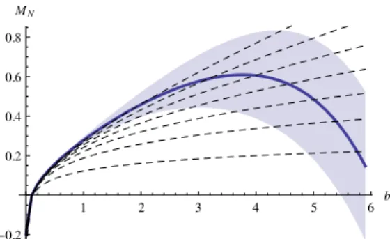
For N → ∞ the sum is divergent, as discussed in section 3.3. In order to define M

we consider the Borel transform of M

as in section 3.3. To define the Borel integral in eq. (3.16), we shift the integration contour, slightly above the real axis. The real part of the integral (i.e. the principal value integral) gives M

, while the imaginary part represents the errorband for this estimation. The explicit expression for the latter is

δM(µ, b) = 2π β

h J

p

µ

b

e

5 6−_2β ¹

0as(µ)

− 1 i

, (4.5)

and the leading behavior at small-b for δM is given by the infrared ambiguity eq. (3.19).

We investigate the convergence of the partial sums of M

to its Borel resummed value

M

, in order to find the scale at which the non-perturbative corrections associated with

renormalons become important. The numerical values of partial sums at µ = 10 GeV and

at several values of b are presented in table 2. The graphical representation of these values

is shown in figure 2. The convergence of the series is perfect (in the sense that it converges

at M

that is far beyond the scope of modern perturbative calculations) for the range of

b . 2 GeV

, it becomes weaker at b ∼ 3 GeV

, and it is completely lost at b & 4 GeV

.

These are the characteristic scales for switching the perturbative and non-perturbative

regimes in D. In other words, the perturbative series can be trustful at b . 2 GeV

, but

completely loses its prediction power for b & 4 GeV

. The number N at which convergence

is lost depends on the value of µ, however the interval of convergence in b is µ-independent,

e.g. at µ = 50 GeV the series converges to M

in the region b . 2 GeV

, but again loses

stability at ∼ 4 GeV

.

JHEP03(2017)002

1 2 3 4 5 6

bT

-0.2 0.2 0.4 0.6 0.8 MN

Figure 2. The dependence of partial sumsMN onb (in GeV⁻¹). The dashed lines representMN

fromN = 1 (bottom line) tillN = 7 (top line). The bold line is the value ofM_∞. The shaded area is the error band ofM_∞ given byδM.

In order to proceed to an estimate of the non-perturbative part of D we write it in the form

D(µ, b) = Z

µ0

dµ

µ

Γ

(µ) + D

(µ

, b) + D

(µ

, b), (4.6) where D

is given by the perturbative expression at µ

scale, D

encodes the non- perturbative part. The parameter µ

depends on b and should be selected such that a

(µ

) is a reasonably small number. The non-perturbative part D

is independent on µ (since the evolution part of D is renormalon-free) but depends on the choice of µ

.

In principle, the best value of the parameter µ

can be extracted from the large-β

calculation. Indeed, the resummation of bubble-diagrams modifies the coupling in the interaction vertex, such that a loop integral appears to be naturally regularized in the infrared region. Practically, the effect of such resummation can be presented as a freezing of the coupling constant at large b. Particularly popular is the b

prescription [44] defined as

µ

= µ

= C

b

(b) , b

(b) =

√ b

p 1 + b

/b

, C

= 2e

. (4.7) At large b the parameter µ

approaches C

/b

, which should be chosen much less then Λ, i.e. b

C

/Λ ∼ 4 GeV

.

For large-b (say b & 3 GeV) the non-perturbative part of D dominates the perturbative one. The large-β

calculation allows to estimate the leading contribution (from the side of small-b’s) to D

from the infrared ambiguity eq. (3.19),

D

(b, µ

) =cΛ

b

g

(b, µ

), (4.8) the function g

should be of order of unity at small-b and it depends on the choice of the scale µ

. Here Λ

is the position of Landau pole and it is expected to be of order O(Λ

) ∼ 250 MeV, which implies

cΛ

= πC

e

2β

Λ

∼ 0.075 GeV

. (4.9)