Calculation of transverse momentum dependent distributions beyond the leading power

JHEP12(2020)145

Published for SISSA by Springer

Received : September 5, 2020 Revised : November 6, 2020 Accepted : November 11, 2020 Published : December 22, 2020

Calculation of transverse momentum dependent distributions beyond the leading power

Valentin Moos and Alexey Vladimirov

Institut für Theoretische Physik, Universität Regensburg, D-93040 Regensburg, Germany

E-mail: Valentin.Moos@physik.uni-regensburg.de, alexey.vladimirov@physik.uni-regensburg.de

Abstract: We compute the contribution of twist-2 and twist-3 parton distribution func- tions to the small-b expansion for transverse momentum dependent (TMD) distributions at all powers of b. The computation is done by the twist-decomposition method based on the spinor formalism for all eight quark TMD distributions. The newly computed terms are accompanied by the prefactor (M ² b ² ) ⁿ and represent the target-mass corrections to the resummed cross-section. For the first time, a non-trivial expression for the pretzelosity distribution is derived.

Keywords: Perturbative QCD, Resummation

ArXiv ePrint: 2008.01744

JHEP12(2020)145

Contents

1 Introduction 1

2 Definitions and conventions 5

2.1 Definition of TMD distributions 5

2.2 Definition of collinear distributions 7

2.3 Spinor formalism 8

3 Twist-decomposition for TMD operators 10

3.1 TMD operator as a series of local operators 11

3.2 Twist decomposition in the spinor formalism 13

3.3 Assembling the final result 16

4 Results and discussion 20

5 Conclusion 24

A Twist-3 part of the operators O _s,n,t 26

B Power corrections for fragmentation functions 27

1 Introduction

Transverse momentum dependent (TMD) distributions extend the parton model, including the transverse motion of hadron’s constituents. Any TMD distribution is a function of two dynamical variables x and b. The variable x is the fraction of hadron’s momentum carried by the parton. The variable b is the transverse distance that is Fourier conjugated to the transverse momentum of parton k _T . In the limit b → 0, which corresponds to integrated or unobserved transverse momentum, a TMD distribution turns to the corresponding collinear parton distribution functions (PDFs) or fragmentation function (FFs). Technically, this relation, which is also known as the matching between TMD parton distribution functions (TMDPDFs) and PDFs (or TMD fragmentation functions (TMDFFs) and FFs), is obtained by the operator product expansion, and its leading power term is very well studied. In the present work, we extend this formalism beyond the leading power term and compute matching of TMDPDFs to PDFs of twist-2 and twist-3 at all powers of b ² -expansion.

The matching of TMDPDFs to PDFs is an important part of the TMD factorization

approach. The review of various aspects of TMD factorization can be found in [1–3]. On the

theory side, the matching establishes the connection with the resummation formalism and

allows interpolation between TMD factorized cross-section and fixed order computations,

see f.i. [4–6]. On the phenomenological side, the matching essentially reduces the parametric

JHEP12(2020)145

freedom for TMD ansatzes. The modern phenomenology of TMD distributions is grounded on the matching relations and demonstrates perfect agreement with a large amount of experimental data [7, 8].

So far, all studies of matching relations were restricted to the leading power term only. The leading power term is the most simple and numerically dominant contribution.

Nonetheless, several aspects make the study of power corrections interesting. First of all, such a study carries a significant amount of methodological novelty. Indeed, the power corrections are generally considered as a complicated field, and their computation is an interesting theoretical task. In this work, we have computed the whole series of power correction with PDFs of twist-2 and twist-3, which is almost unprecedented. Methodolog- ically, the closest example of similar computation is the computation of kinematic power corrections to Deeply Virtual Compton Scattering (DVCS) made by Braun and Manashov in ref. [9]. The second point of interest is the derivation of the matching relations for polar- ized TMD distributions. For many TMD distributions already, the leading power matching involves twist-3 functions and requires a non-trivial computation. The computations for different TMDPDFs have been made by different methods in refs. [10–13]. In ref. [14], all polarized TMDPDFs were systematically computed in a single scheme, and the agreement with previous computations had been shown. However, all these computations were unable to find the non-trivial matching of the pretzelosity distribution, which is derived for the first time in this work. The third point of interest is the comparison of the derived power corrections to the extracted ones. There are many examples, where the part of the power correction proportional to twist-2 PDFs (Wandzura-Wilczek approximation) is numerically dominant [15, 16]. However, there are also known cases of opposite behavior [16]. In this work, we demonstrate that Wandzura-Wilczek-type terms produce only a small part of the k _T -profile of TMD distributions, and the contribution of higher twist PDFs is essential.

The forth point of interest is the target-mass dependence of TMD distributions. At higher powers of small-b series, the target mass is the only scale that compensates the dimension of b ⁿ for twist-2 and twist-3 distributions. Thus, the corrections derived here are target-mass corrections ∼ (M ² b ² ). Their knowledge is essential since much of the experimental data is measured on nuclei.

Formally, the matching is obtained by operator product expansion of the transverse momentum dependent operator (defined explicitly in (3.1)) at small values of b. The latter has the schematic form

O ^TMD (z, b) = O 2 (z) + b µ O ^µ 3 (z) + b µ

b µ

2 O ^µ 4

^µ

(z) + . . . =

∞

X

n=0

b µ

. . . b µ

n! O ^µ n+2

^...µ

(z), (1.1) where z is the distance among the fields of the operator along the light-cone. The operators O n (z) are light-cone operators with the collinear twist n. For example, the leading power operator is O 2 (z) ∼ q(zn)[zn, ¯ 0]q(0), where n is the light-cone vector, [a, b] is the straight gauge link, and q is the quark field. Each operator O n is an integral convolution of a coefficient function and an actual quantum-field operator. The coefficient functions for O 2

are all known at next-to-leading order (NLO) in α s -expansion [17, 18], and NNLO [5, 19–

21]. The leading power coefficient function for unpolarized distribution has been recently

JHEP12(2020)145

computed at N ³ LO [22, 23]. Beyond the leading power the information is sparse. The tree order matching for O 3 has been derived in [14], see also [10–13] for particular cases.

The only NLO computation for O 3 is made for the Sivers function [24]. In this work, we derive only the tree order matching, ignoring the α _s -suppressed terms in the coefficient functions. For that reason, we do not specify the renormalization scales and omit the corresponding arguments.

The operators with the collinear twist n can be presented as a sum of operators with different geometrical twists,

O n (z) =

n

X

t=2

C _t (z; {y}) ⊗ O _t ({y}), (1.2)

where we omit indices µ 1 . . . µ n for brevity. For shortness, we call this procedure as twist- decomposition. Generally, operators O _t depend on many spatial points, which are parame- terized by a set of variables {y}. They are mapped to the single variable z by the integral convolution ⊗. The geometric twist has a strict definition as the “dimension minus spin”

of the operator. Operators with different geometrical twists have different transformation properties and thus represent independent physical observables. The matrix elements of operators with a given geometrical twist define a self-contained set of PDFs. Such a set of PDFs does not mix with other sets, and their evolution is autonomous. For the intro- duction to the twist decomposition see e.g. [25, 26], the review of modern development can be found in [9]. Therefore, the central task is to derive the twist-decomposition for each operator on the right-hand-side (r.h.s. ) of (1.1). In turn, the small-b expansion of TMDPDFs in terms of collinear PDFs is obtained by evaluating the matrix element over the derived operator relation.

In the case of FF, the twist-decomposition operation is not well defined. The main reason is the absence of a local expansion for fragmentation operators. In ref. [27] it has been shown that OPE for FF is defined up to terms that satisfy the Laplace equation (for the twist-2 part). Therefore, alternative methods such as differential equations [27], Feynman diagram correspondences [19, 28–30] and Lorentz invariant relations [13], should be used. For that reason, we do not consider the matching of TMDFFs to FFs in the present work. For an interested reader, we present some discussion on power corrections for TMDFF in appendix B.

In this work, we compute only quark TMD distributions, since they are of the prime practical interest. In total, there are eight TMDPDFs in the leading term of the factoriza- tion theorem [31]. They can be split into two classes with respect to the structure of match- ing relations. Four distributions, namely f ₁ (unpolarized), g _1L (helicity), h ₁ (transversity) and h ^⊥ _1T (pretzelosity) have contributions of only even collinear twists

F _even (x, b) = f (x) + M ² b ²

4

X

t=2

C _t ⁽²⁾ (x) ⊗ T _t + (M ² b ² ) ²

6

X

t=2

C _t ⁽⁴⁾ (x) ⊗ T _t + . . . , (1.3)

where T t is a collinear distribution of twist-t and T ₂ (x) = f (x) is the twist-2 PDF. Another

four distributions, namely f _1T ^⊥ (Sivers), g _1T (worm-gear T), h ^⊥ ₁ (Boer-Mulders) and h ^⊥ _1L

JHEP12(2020)145

1 b

b

b

f (x) f (x) f (x) f (x)

T

T

T

T

T

T

T

T

T

T

. . . . . . . . . . . . . . . . . . . TMD distributions f

, g

, h

, h

Collinear distributions Power

1 b

b

b

f(x) f(x) f(x) f(x)

T

T

T

T

T

T

T

T

T

T

T

T

. . . . . . . . . . . . . . . . . . . . . . TMD distributions f

, g

, h

, h

Collinear distributions Power

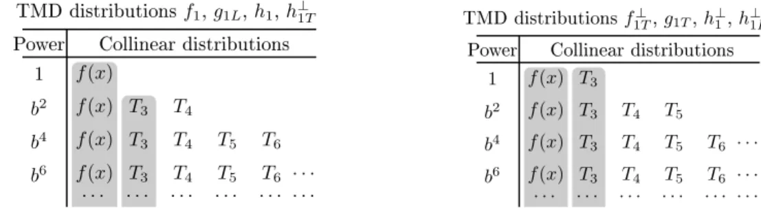
Figure 1. Ordering of parton distributions in the small-b series for TMD distributions (1.3) (left) and (1.4) (right). f (x) denotes the ordinary PDFs. T

denotes the parton distribution of twist-n, which is generally a function of several variables. The gray boxes designate the terms computed in this work.

(worm-gear L), have contributions of only odd collinear twists F _odd (x, b) =

3

X

t=2

C _t ⁽¹⁾ (x) ⊗ T _t + M ² b ²

5

X

t=2

C _t ⁽³⁾ (x) ⊗ T _t + . . . . (1.4) The graphical representation of these sums is shown in figure 1. The parameter M in (1.3), (1.4) is the mass of the hadron, which is inserted such that all coefficient functions C _t ⁽ⁿ⁾ are dimensionless. The sums (1.3) and (1.4) can be reorganized by collecting together distributions of particular twist. For example, equation (1.3) takes the form

F _even (x, b) =

∞

X

n=0

(M ² b ² ) ⁿ C ₂ ⁽ⁿ⁾ (x) ⊗ f (1.5)

+

∞

X

n=1

(M ² b ² ) ⁿ C ₃ ⁽ⁿ⁾ (x) ⊗ T ₃ +

∞

X

n=1

(M ² b ² ) ⁿ C ₄ ⁽ⁿ⁾ (x) ⊗ T ₄ + . . . .

In the present work, we derive the first and the second terms of this sum for all eight TMD distributions. In figure 1, the shaded areas show the corresponding terms.

To perform this computation, we use the technique inherited from [32, 33], where it was used for the analyses of twist-4 operators. The technique is based on the local equivalence of the Lorentz transformation group to SL(2,C) group (so-called spinor formalism) [34].

Within the spinor formalism, the twist-decomposition can be elegantly formulated as the

action of a certain spinor-differential operator (see section 3.2). In ref. [9] this method

has been used to derivate kinematic power corrections (t/Q ² ) in deeply-virtual Compton

scattering. In contrast to ref. [9], TMD operators are essentially non-local. They contain

the gauge link along a staple contour. To overcome this difficulty, we introduce a formal

local expansion for the TMD operator. To our best knowledge, it is the first time when

the series of local operators successfully describes the infinite staple contours. Almost all

expressions presented in this article are novel. Only some of them, namely b ⁰ - and b ¹ -terms,

can be found in literature and agree with it. Additionally, we demonstrate that the series

of corrections for the unpolarized TMDPDF f ₁ can be derived differently using the results

of ref. [35] and also agrees with it.

JHEP12(2020)145

The article is organized as follows. In section 2 we articulate all definitions used in our work. This is an important part because we deal with functions that do not have a common definition such as polarized distributions and PDFs of twist-3. In section 2.3 we specify the conventions for the spinor formalism used in our work. Section 3 is devoted to the detailed description of the computation method. It is split into three subsections in accordance with three principal stages of the computation:(1.1), (1.2) and (1.3), (1.4).

So, in section 3.1 the expansion (1.1) of the TMD operator in the series of (local) collinear operators is described. In section 3.2 we explain the method of the twist-decomposition and derive it for TMD operators (1.2), with results for twist-3 part presented in the appendix A.

The particularities of the computation of matrix elements for twist-decomposed operators are given in section 3.3. The result of the computation and the discussion are given in section 4.

2 Definitions and conventions

In this work, we operate with eight TMD distributions. Three of them have leading match- ing onto collinear twist-2 distributions, and four onto collinear twist-3 distributions, and one (pretzelosity) matches onto collinear twist-4 distribution. They essentially depend on the conventions related to P-odd structures, such as Levi-Civita tensor, γ ⁵ , etc. An additional set of conventions is brought by the spinor formalism which is used for the twist-decomposition. There is no commonly accepted convention for all these subjects in the literature, e.g. compare conventions in refs. [12–14, 25, 34, 36–38]. Nicely, the final re- sult is mostly independent on these agreements, because it is the relation between physical distributions. Nonetheless, they play an important role in the intermediate steps. In order to structure the presentation we collect all used definitions and conventions in this section.

2.1 Definition of TMD distributions

The light-cone decomposition plays the central role. It is defined by two light-like vectors n ^µ and ¯ n ^µ (n ² = ¯ n ² = 0, (n¯ n) = 1). We use the ordinary notation of vector decomposition v ^µ = v ⁺ n ¯ ^µ + v ⁻ n ^µ + v _T ^µ , (2.1) where v ⁺ = (nv), v ⁻ = (¯ nv), and v _T is the transverse component (v _T n) = (v _T n) = 0. ¯ In what follows, the direction ¯ n ^µ is associated with the large-component of the hadron momentum p ^µ ,

p ^µ = p ⁺ ¯ n ^µ + n ^µ 2

M ²

p ⁺ , (2.2)

where M is the mass of the hadron (p ² = M ² ). It is important, that the hadron’s mo- mentum does not have a transverse component, which gives the physical definition of the transverse plane. The spin of the hadron is parameterized by the spin-vector S ^µ , (S ² = −1, (pS ) = 0). Its light-cone decomposition is

S ^µ = λ p ⁺

M n ¯ ^µ − λ M

2p ⁺ n ^µ + s ^µ _T , (2.3)

JHEP12(2020)145

where the λ is the helicity of the hadron, and s ^µ _T is the transverse component of the spin, s ² _T = λ ² − 1.

The generic quark TMDPDF is defined as Φ _ij (x, b) =

Z dz

2π e ^−ixzp

(2.4)

×hp, S|¯ q _j (zn + b) [zn + b, ∓∞n + b][∓∞n + b, ∓∞n][∓∞n, 0]q _i (0)}|p, Si, where the vector b ^µ is a transverse vector, (bp) = 0. The Wilson lines in the definition (2.4) are straight Wilson lines. Rigorously, one should add the T- and anti-T-ordering within the TMD operator. However, for the parton distributions (in contrast to fragmentation functions) it can be safely omitted (see e.g. discussion in [24]). TMDPDFs that appear in different processes have Wilson lines pointing into different direction, which is indicated by ∓∞n in (2.4). So, the TMD distributions which appear in semi-inclusive deep-inelastic scattering (SIDIS) have Wilson lines pointing to +∞n, while in Drell-Yan they point to

−∞n. In the following, we distinguish these cases, and the upper sign refers to the Drell- Yan case, whereas the lower sign refers the SIDIS case.

The open indices (ij) of the TMD operator in eq. (2.4) are to be contracted with different gamma-matrices, which we denote generically as Γ,

Φ ^[Γ] = 1

2 Tr (ΦΓ) . (2.5)

There are only three Dirac structures that appear in the leading term of the TMD factor- ization theorem, these are Γ = {γ ⁺ , γ ⁺ γ ₅ , iσ ^α+ γ ₅ }. Here, the index α is transverse and

σ ^µν = i

2 (γ ^µ γ ^ν − γ ^ν γ ^µ ), γ 5 = iγ ⁰ γ ¹ γ ² γ ³ = −i

4! _µναβ γ ^µ γ ^ν γ ^α γ ^β , (2.6) with ⁰¹²³ = − ₀₁₂₃ = 1. In the naive parton model interpretation, these gamma-structures are related to the observation of unpolarized (γ ⁺ ), longitudinally polarized (γ ⁺ γ ⁵ ) and transversely polarized (iσ ^α+ _T γ ⁵ ) quarks inside the hadron. The standard parameterization of leading TMDPDFs in the position space reads

Φ ^[γ

^] (x, b) = f ₁ (x, b) + i ^µν _T b _µ s _{T ν} M f _1T ^⊥ (x, b), (2.7) Φ ^[γ

^γ

^] (x, b) = λg _1L (x, b) + ib µ s ^µ _T M g _1T (x, b), (2.8) Φ ^[iσ

^γ

^] (x, b) = s ^α _T h 1 (x, b) − iλb ^α M h ^⊥ _1L (x, b)

+i ^αµ _T b _µ M h ^⊥ ₁ (x, b) − M ² b ² 2

g _T ^αµ

2 − b ^α b ^µ b ²

!

s _{T µ} h ^⊥ _1T (x, b). (2.9) The tensors g _T ^µν and ^µν _T are defined as

g ^µν _T = g ^µν − n ^µ n ¯ ^ν − n ¯ ^µ n ^ν , ^µν _T = ^−+µν , (2.10)

such that g _T ¹¹ = g _T ²² = −1, ¹² _T = − ²¹ _T = 1, and the rest components are zero. The definition

of the TMDPDFs coincides with the conventional one in [14, 36, 39]. In the following, we

JHEP12(2020)145

also compare to refs. [9, 33, 37], where the definitions of and s _T have opposite sign, and ref. [14], where the definitions of and T have opposite sign (so, component-wise the tensor ^µν _T is the same). TMDPDFs defined in (2.7)–(2.9) are dimensionless functions which depend only on the modulus of b, but not on the direction. The conventional names for them are (see e.g. [36, 39]): unpolarized (f 1 ), Sivers (f _1T ^⊥ ), helicity (g 1L ), worm- gear T (g _1T ), transversity (h ₁ ), worm-gear L (h ^⊥ _1L ), Boer-Mulders (h ^⊥ ₁ ) and pretzelosity (h ^⊥ _1T ) distributions.

The position space representation of TMD distribution is advantageous, because the TMD evolution is multiplicative in the position space. For that reason, the phenomeno- logical studies that incorporate the TMD evolution are made in the position space, for the most recent examples see [7, 8]. TMD distributions in the momentum space are obtained by the Fourier transformation

Φ ^[Γ] (x, p T ) =

Z d ² b

(2π) ² e ^−i(bp

⁾ Φ ^[Γ] (x, b). (2.11) The transformation rules for particular TMD distributions can be found in refs. [14, 39].

2.2 Definition of collinear distributions

The collinear distributions of twist-2 are defined as [25]

hp, S|¯ q(zn)[zn, 0]γ ⁺ q(0)|p, Si = 2p ⁺ Z

dxe ^ixzp

f ₁ (x), (2.12) hp, S|¯ q(zn)[zn, 0]γ ⁺ γ ⁵ q(0)|p, Si = 2λp ⁺

Z

dxe ^ixzp

g ₁ (x), (2.13) hp, S|¯ q(zn)[zn, 0]γ ⁺ iσ ^α+ γ ⁵ q(0)|p, Si = 2s ^α _T p ⁺

Z

dxe ^ixzp

h ₁ (x), (2.14) where index α is transverse. These distributions are known as unpolarized (f 1 ), helicity (g ₁ ) and transversity (h ₁ ) PDFs. The variable x belongs to the range [−1, 1] and for x > 0 (x < 0) PDFs are interpreted as probability densities for (anti-)quarks.

There is no standard definition for the collinear distributions of twist-3. Here, we use the definition used in [14]. We define

hp, S|g q(z ¯ ₁ n)F ^µ+ (z ₂ n)γ ⁺ q(z ₃ n)|p, Si (2.15)

= 2 ^µν _T s _νT (p ⁺ ) ² M Z

[dx]e ^−ip

^(z

^x

^+x

^z

^+x

^z

⁾ T(x ₁ , x ₂ , x ₃ ),

hp, S|g q(z ¯ 1 n)F ^µ+ (z 2 n)γ ⁺ γ ⁵ q(z 3 n)|p, Si (2.16)

= 2is ^µ _T (p ⁺ ) ² M Z

[dx]e ^−ip

^(z

^x

^+x

^z

^+x

^z

⁾ ∆T (x 1 , x 2 , x 3 ),

hp, S|g q(z ¯ ₁ n)F ^µ+ (z ₂ n)iσ ^α+ γ ⁵ q(z ₃ n)|p, Si (2.17)

= 2 ^µα _T (p ⁺ ) ² M Z

[dx]e ^−ip

^(z

^x

^+x

^z

^+x

^z

⁾ δT (x 1 , x 2 , x 3 ) +2iλg ^µα _T (p ⁺ ) ² M

Z

[dx]e ^−ip

^(z

^x

^+x

^z

^+x

^z

⁾ δT _g (x ₁ , x ₂ , x ₃ ),

JHEP12(2020)145

where we omit Wilson lines that connect the fields in operators for brevity. The definition of the distributions T and ∆T coincides with [40] and [37], taking into account the difference in conventions for the -tensor (explained after (2.10)). In ref. [40] one can also find comparison with other definitions. The integration measure [dx] is defined as

Z

[dx] = Z 1

−1

dx ₁ dx ₂ dx ₃ δ(x ₁ + x ₂ + x ₃ ). (2.18) The delta-function in this measure reflects the independence of the matrix element on the global position (z 1 + z 2 + z 3 ) of the field operator. Due to the delta-function in the measure, the distributions of twist-3 effectively depends on only two variables. Nonetheless, it is convenient to keep all three variables x 1,2,3 as independent. It reveals the symmetry properties [14]

T (x ₁ , x ₂ , x ₃ ) = T (−x ₃ , −x ₂ , −x ₁ ), ∆T (x ₁ , x ₂ , x ₃ ) = −∆T(−x ₃ , −x ₂ , −x ₁ ), (2.19) δT (x 1 , x 2 , x 3 ) = δT (−x ₃ , −x ₂ , −x ₁ ), δT g (x 1 , x 2 , x 3 ) = −δT _g (−x ₃ , −x ₂ , −x ₁ ). (2.20) Each range of x 1,2,3 ≶ 0 has a specific partonic interpretation [25].

2.3 Spinor formalism

The twist-decomposition for local operators consists in the decomposition of tensors with many indices into irreducible representations of the Lorentz group SO(3,1). This procedure is greatly simplified in the spinor formalism. The spinor formalism is used in many parts of quantum field theory, for a review see [34, 38]. Here we remind only of the properties that are necessary for the current work.

The spinor formalism is grounded on the local isomorphism of the Lorentz group to the group of complex unimodular matrices SL(2,C). The isomorphism is realized by the map of a four-vector to a hermitian matrix by the rule

x α α ˙ = x µ σ _α ^µ _{α ˙} , (2.21)

where σ ^µ = {1, σ ¹ , σ ² , σ ³ } with σ ⁱ being the Pauli matrix. The scalar product of any two vectors is x _µ y ^µ = x _{α α ˙} y ^{αα ˙} /2. In the spinor formulation one must distinguish dotted and undotted indices because they are related to conjugated representations, (u _α ) ^∗ = ¯ u _{α ˙} . The scalar product of two spinors is defined as

(uv) = −u ^α v ^β _αβ = −(vu), (¯ u¯ v) = −¯ u α ˙ v ¯ β ˙ ^{α ˙ β ˙} = −(¯ v¯ u), (2.22) where ₁₂ = − _{˙1 ˙2} = 1 as in refs. [9, 32, 33].

The light-like vectors n and ¯ n in the spinor formalism can be written as

n _{α α ˙} = λ _α λ ¯ _{α ˙} , n ¯ _{α α ˙} = µ _α µ ¯ _{α ˙} , (2.23) where λ and µ are independent spinors normalized as (¯ λ¯ µ)(µλ) = 2. The spinors λ and µ form the basis, which can be used to decompose any tensor. In particular, the decomposi- tion (2.1) for an arbitrary four-vector is

x _{α α ˙} = λ _α λ ¯ _{α ˙} x ⁻ + µ _α µ ¯ _{α ˙} x ⁺ − λ _α µ ¯ _{α ˙} x _T − µ _α λ ¯ _{α ˙} x ¯ _T , (2.24)

JHEP12(2020)145

where x _T and ¯ x _T are transverse components. x _T and ¯ x _T are complex numbers, such that (x T ) ^∗ = ¯ x T and −2x _T x ¯ T = g _T ^µν x µ x ν < 0. The explicit expression for basis spinors and vector components is not important for present work. ¹

The Dirac bi-spinors are written as composition of two-component spinors q ¯ = χ ^β , ψ ¯ α ˙

, q = ψ _α χ ¯ ^{β ˙}

!

. (2.25)

The decomposition of these spinors in the basis (2.23) is ψ _α = λ _α ψ − − µ _α ψ ₊

(µλ) , ψ ¯ _{α ˙} =

λ ¯ _{α ˙} ψ ¯ − − µ ¯ _{α ˙} ψ ¯ ₊

(¯ λ¯ µ) , (2.26)

where ψ ₊ = (λψ), ψ − = (µψ), etc. In the same way, we write down the decomposition of the gluon-strength tensor,

F _{α α,β ˙} β ˙ = 2(f αβ _{α ˙} β ˙ − αβ f ¯ _{α ˙} β ˙ ), (2.27) where f _αβ and ¯ f _{α ˙ β ˙} are symmetric tensors, ¯ f = f ^† . In our computation we face only the gluon strength-tensor with one index transverse, and another contracted with the vector n. The decomposition of such a tensor is

F α α,+ ˙ = λ α ¯ λ α ˙

f +−

(µλ) + f ¯ +−

(¯ λ¯ µ)

!

− µ α ¯ λ α ˙

f ++

(µλ) − λ α µ ¯ α ˙

f ¯ ++

(¯ λ¯ µ) , (2.28) where f ₊₊ = f _αβ λ ^α λ ^β , f +− = f _αβ λ ^α µ ^β , etc. The first term in (2.28) corresponds to F −+

components, whereas the last two terms describe F µ+ with µ being transverse index.

Using the definitions (2.25) and (2.26) we write down the decompositions for the bi- spinor combinations. They are

qγ ¯ ⁺ q = ¯ ψ ₊ ψ ₊ + χ ₊ χ ¯ ₊ , qγ ¯ ⁺ γ ⁵ q = − ψ ¯ ₊ ψ ₊ + χ ₊ χ ¯ ₊ , (2.29) qiσ ¯ ^{(α α)+ ˙} γ ⁵ q = −2 µ ^α λ ¯ ^{α ˙}

(µλ) χ ₊ ψ ₊ + λ ^α µ ¯ ^{α ˙} (¯ λ¯ µ)

ψ ¯ ₊ χ ¯ ₊

!

, (2.30)

where the order of the fields on l.h.s. and r.h.s. is preserved. Let us note that only “plus”

components of quark fields appear in eqs. (2.29), (2.30). It is not accidental, but is part of definition for the leading power TMD distributions. The components ψ + , χ + , etc, are known as “good” components of quark field in contrast to “bad” components (ψ − , χ − , etc) [25]. The operators made with only good components (including also good components of the gluon field f ++ and ¯ f ++ ) are called quasi-partonic operators. Their geometrical twist coincides with their collinear twist. All operators of twist-2 and twist-3 can be expressed as quasi-partonic operators with the help of EOMs [35].

1

An example of explicit realization for basis spinors with our conventions is λ

= (2

, 0), µ

= (0, 2

), λ ¯

= (0, −2

) and ¯ µ

= (2

, 0), assuming the standard representation for Pauli matrices. With this choice the components of the vector decomposition (2.24) are

x

= x

± x

√ 2 , x

= x

+ ix

√ 2 , x ¯

= x

− ix

√ 2 .

JHEP12(2020)145

The last ingredient needed for our computation are the equations of motion (EOMs) for the quark field 6 Dq = 0 (for massless quarks). In the spinor notation EOMs read D ^{αα ˙} ψ _α = 0, χ ^α ← −

D _{α α ˙} = 0, and similar for other spinors. Contracting these equations with the basis spinors one obtains EOMs for particular components. For our purposes we need the following EOMs

D _λ ¯ λ ψ − = D _µ λ ¯ ψ + , D _λ ¯ λ χ ¯ − = D λ¯ µ χ ¯ + , (2.31) ψ ¯ −

←−− D _λ ¯ λ = ¯ ψ +

←−− D λ¯ µ , χ −

←−− D _λ ¯ λ = χ +

←−− D _µ ¯ λ , (2.32) where D _ab = D _{α α ˙} a ^α b ^{α ˙} .

3 Twist-decomposition for TMD operators

In this section, we present the details of the twist-decomposition procedure. The method is based on the results of refs. [32, 33], to which we refer for extended details and the theory foundation. There are three principal steps of the computation:

1. The operator is presented as a series of local operators.

2. Local operators are sorted by irreducible representation of Lorentz group (twists), and simplified using EOMs.

3. The series of operators with the same twists are summed back into the non-local form.

This is a rather traditional approach. Examples of such evaluation for collinear operators can be found in refs. [25, 32, 33, 35, 41, 42]. For TMD operators each of these steps has a certain particularity. Let us list these particularities, and explain the methods that were used to resolve them:

1. The TMD operator has the staple-shaped gauge link with infinite length. Therefore, it is not possible to present it as a series of local operators directly. We regularize the TMD operator by truncation of the length of Wilson lines by the parameter L. As the result TMD operators are presented as a limit of triple series of local operators (3.11).

2. The local operators for TMDPDFs have three sets of indices (s, n, t). They correspond to the number of light-cone derivatives acting on the anti-quark field (s), the number of transverse derivatives (n) and the number of light-cone derivatives acting on the quark field (t). Such structure somewhat complicates the twist-decomposition alge- bra, in comparison to the case of local operators that describe (Mellin moments of) collinear distributions, where all indices are alike. To simplify the twist-decomposition procedure we use the method introduced in refs. [32, 33], which is based on the spinor formalism. This method allows to perform the twist-decomposition for the most general operators using only differential operations (compare to refs. [14, 43] where off-light-cone generalizations of operators and integral equations are used, ref. [35]

where the differential equation are used, refs. [41, 42] where an explicit procedure of

index symmetrization is performed).

JHEP12(2020)145

3. The summation of the series of definite-twist operators is performed for the matrix- elements, i.e. for distributions. It simplifies certain steps of the computation, and helps to resolve potential ambiguities in the limit L → ∞.

The following sections give the details for each step of this order. The results of the computation are collected in section 4. We stress that such an approach is suitable only for TMDPDFs, but does not apply for TMDFF. The discussion for TMDFFs case is given in appendix B.

3.1 TMD operator as a series of local operators Let us introduce the TMD operator in the form

O ^Γ _TMD (z, b) = ¯ q(zn + b)[zn + b, ∓∞n + b][∓∞b + b, ∓∞n]Γ[∓∞n, 0]q(0). (3.1) The upper(lower) sign corresponds to Drell-Yan(SIDIS) induced TMD. The transverse gauge link [∓∞n + b, ∓∞n] ensures the explicit gauge invariance of the operator.

At tree-order quantum fields can be treated as classical fields, and thus the small-b expansion is an ordinary Taylor expansion. It is convenient to write it in the form (1.1)

O ^Γ _TMD (z, b) =

∞

X

n=0

b ^µ

. . . b ^µ

n! O ^Γ µ

...µ

(z), (3.2) with

O ^Γ µ

...µ

(z) = ¯ q(zn)[zn, −∞n] ←−−

D µ

. . . ←−−

D µ

Γ[−∞n, 0]q(0), (3.3) where D µ is the covariant derivative

←− D µ = ∂ µ + igA µ , −→

D µ = ∂ µ − igA µ . (3.4)

The operators on r.h.s. of (3.2) have collinear twist n+2, which follows from their dimension.

At the same time, these operators do not have a definite geometrical twist, and therefore, their matrix element is a complicated composition of collinear distributions with different properties. Our goal is to perform the twist-decomposition and express these operators in terms of operators with definite geometrical twist.

In contrast to collinear operators, the TMD operator (3.1) spans an infinite range along the light cone. It is the most famous feature of TMD operators, and it leads to many physical effects, such as rapidity divergences [44], double-scale nature of TMD evolution [40]

and the sign-change of P-odd distributions [45]. In the b → 0 limit, the infinite Wilson lines are partially compensated, due to the transitivity property of Wilson lines. For example, at n = 0 the operator (3.3) simplifies to

O ^Γ (z) = ¯ q(zn)[zn, −∞n]Γ[−∞n, 0]q(0) = ¯ q(zn)[zn, 0]Γq(0). (3.5) However, already at n = 1 the infinities enter the expressions,

O ^Γ µ (z) = ¯ q(z) ←−

D _µ [zn, 0]Γq(0) + ig Z z

∓∞

dσ q(zn)[zn, τ n]F ¯ _µ+ (τ n)[τ n, 0]Γq(0), (3.6)

JHEP12(2020)145

where F _µν = ig ⁻¹ [D _µ , D _ν ] is the gluon-strength tensor. The operators on the r.h.s. of these formulas are ordinary collinear operators. The infinite size of the TMD operator is reflected in the limit of integration in the last term of (3.6).

In equation (3.6), the twist-decomposition of operators is straightforward. In ref. [14], this decomposition has been made for all leading Γ-structures. Despite such method is intuitive and explicitly reveals features of the TMD operator, it became algebraically complicated for higher n. The main source of complication is new classes of non- local operators introduced with increasing of n. For instance, at n = 2 the oper- ators like ¯ q(zn)F _+µ (τ ₁ n)F _+ν (τ ₂ n)q(0), ¯ q(zn)[D _ν F _µ+ (τ n)]q(0), ¯ q(zn)F _µ+ (τ n)D _ν q(0) and q(zn) ¯ ←−

D µ

− →

D ν q(0) appear. The first operator is quasi-partonic and has geometric twist-4, whereas other operators have indefinite geometric twist and should be processed using EOMs to extract twist-2 and twist-3 components. At n = 3 the operators with two and three derivatives in different composition arise. Each of these new cases requires individual investigation to extract the lower geometrical twist component. Therefore, this approach is ineffective.

To avoid these complications we operate directly with the operators (3.2) with the help of the following formal procedure. We introduce the regularized operator,

O _TMD ^Γ (z, b; L) = ¯ q(zn + b)[zn + b, Ln + b][Ln + b, Ln]Γ[Ln, 0]q(0). (3.7) This operator turns to the TMD operator in the limit L → ∓∞. Note, that the same regularization also regularizes rapidity divergences and can be used to derive the non- perturbative definition of the Collins-Soper kernel [46]. In the regularized form the opera- tor (3.3) is

O ^Γ _µ

_...µ

(z; L) = ¯ q(zn)[zn, Ln] ←−−

D µ

. . . ←−−

D µ

Γ[Ln, 0]q(0). (3.8) This operator can be written as the formal expansion,

O ^Γ µ

...µ

(z; L) =

∞

X

s,t=0

z ^s ₁ z ^t ₂ s!t! q ¯ ←−

D ₊ ^s ←−−

D _µ

. . . ←−−

D _µ

Γ −→

D ₊ ^t q(Ln), (3.9) where all fields of the operator are positioned at the point Ln and

z ₁ = z − L, z ₂ = −L. (3.10)

In this way the TMD operator (3.1) is presented as a triple sum O _TMD ^Γ (z; b) = lim

L→∓∞

∞

X

s,t,n=0

z ₁ ^s s!

z ^t ₂ t!

1

n! O ^Γ _s,n,t (Ln), (3.11) with

O ^Γ _s,n,t = ¯ q ←−

D ₊ ^s (b · ← − D ) ⁿ Γ −→

D ₊ ^t q. (3.12)

The r.h.s. of this expression is suitable for the twist-decomposition procedure.

JHEP12(2020)145

The limit L → ∓∞ must be taken with caution. In particular, the summation over s and t must be done before the limiting operation, and the result of the summation should be presented in the form that does not allow any ambiguity. The significant simplification of the summation procedure comes from the possibility to neglect the total derivative terms.

The matrix element of a total-derivative operator is proportional to the momentum transfer, hp ₁ |∂ _µ O|p ₂ i = i(p ₁ − p ₂ ) _µ hp ₁ |O|p ₂ i. (3.13) Consequently, the total derivative operators do not contribute to TMDPDFs, and we ne- glect such terms in the following. After elimination of the total derivative contribution the result of summation is independent on L in many cases. The simplest example is n = 0 case, where

∞

X

s,t=0

z ₁ ^s s!

z ₂ ^t

t! O ^Γ _s,0,t =

∞

X

s,t=0

z ₁ ^s s!

(−z ₂ ) ^t

t! O _s+t,0,0 ^Γ + total der. (3.14)

=

∞

X

s=0

(z ₁ − z ₂ ) ^s

s! O ^Γ _s,0,0 + total der. ,

with z 1 − z 2 = z being independent on L. Only in the cases of Sivers and Boer-Mulders functions the limit L → ∓∞ is not so straightforward. Let us also note that the direction of the limit is the only difference between Drell-Yan (L → −∞) and SIDIS (L → +∞) cases in the representation (3.11).

3.2 Twist decomposition in the spinor formalism

The twist-decomposition for the local operators (3.12) is equivalent to the decomposition into irreducible representation of Lorentz group. The highest spin representation (com- pletely symmetric and traceless in all vector indices) corresponds to the twist-2 term. The next representation (anti-symmetric for one pair of indices, and symmetric and traceless for all other vector indices) corresponds to the twist-3 term. Despite the twist-decomposition is a straightforward operation, it is algebraically complicated, especially for the operators with many transverse indices (for which one has to subtract traces). Additional compli- cation is caused by EOMs, which could relate operators. In refs. [32, 33] it was observed that the decomposition of higher-indices tensors over irreducible representations is simpler in the spinor representation. The main simplification comes from the anti-symmetry of the scalar product (2.22). Due to it, any symmetric tensor (in the spinor space) is automat- ically traceless. The irreducible representations in SL(2,C) group are obtained by simple symmetrization or anti-symmetrization of spinor indices. This operation can be presented as a differential operator, what essentially simplifies the algebra. Here we present this methods in a slightly modified form, which makes its application more explicit.

Let us consider an operator where all open indices are contracted with basis spinors:

O Λ = Λ ^α...β ₁ (λ, µ)Λ ^α... ₂ ^{˙ β ˙} (¯ λ, µ) ¯ O _{α...β; ˙ α...} β ˙ , (3.15)

where Λ _1,2 are monomials of basis spinors, for example (3.27). The lowest geometrical

twist contribution can be obtained by the symmetrization of dotted and undotted indices

JHEP12(2020)145

(independently). It can be done for the operator, or for the tensor Λ. Due to the irre- ducibility of the representation the symmetry properties of one are mapped to another in the convolution. The symmetrization of the tensor Λ can be made by the following operation

S n Λ ^α...β (λ, µ) = µ∂

∂λ

n λ∂

∂µ n

Λ ^α...β (λ, µ), (3.16)

where

µ∂

∂λ = µ ^α ∂

∂λ ^α , λ∂

∂µ = λ ^α ∂

∂µ ^α , (3.17)

and n is the number of spinors µ in the tensor Λ. The logic behind the construction is the following. First, the action of derivatives (λ∂)/(∂µ) replaces all µ’s by λ’s. The resulting tensor is automatically symmetric in indices. Next, the derivatives (µ∂)/(∂λ) replace entries of λ by µ in the fully symmetric fashion.

The higher twist representations are obtained by anti-symmetrizing pairs of indices.

So, the anti-symmetrization of a single pair can be done by the operator A 1 = (µ ^α λ ^β − λ ^α µ ^β ) ∂

∂µ ^α

∂

∂λ ^β = µ∂

∂µ λ∂

∂λ − µ∂

∂λ λ∂

∂µ + µ∂

∂µ , (3.18)

where (µ∂)/(∂µ) and (λ∂)/(∂λ) defined similarly to (3.17). The symmetrization of n pairs is done by

A n = (µ ^α

λ ^β

− λ ^α

µ ^β

) . . . (µ ^α

λ ^β

− λ ^α

µ ^β

) ∂

∂µ ^α

∂

∂λ ^β

. . . ∂

∂µ ^α

∂

∂λ ^β

. (3.19) The operators S and A commute, [A n , S _k ] = 0, for any n and k. The complete decompo- sition of a tensor with n entries of spinor µ then reads

Λ ^α...β (λ, µ) =

n

X

k=0

c _n,k A _k S _n−k Λ ^α...β (λ, µ), (3.20) where c n,k are numbers depending on the tensor Λ. Each term in this sum corre- sponds to an irreducible representation, and the operators S n−k A _k are projectors onto this representation.

To find the coefficients c n,k of the decompositions (3.20) we need to normalize the operators A _k S _n , such that (A _k S _n ) ² = A _k S _n . For example, for the symmetrization operator we compute

S _n S _n = n!S _n

n−1

Y

m=0

λ∂

∂λ + µ∂

∂µ − m

. (3.21)

The operators (λ∂)/(∂λ) and (µ∂)/(∂µ) count the number of λ’s and µ’s in the tensor.

Therefore, S n is indeed the projector to the totally symmetric representation, and the

normalization factor for S n is (N − n)!/(n!N !) where N is the total number of indices

of the tensor. In the same way, one can check that A _n S _k are projectors, and find the

JHEP12(2020)145

corresponding normalization factors. For our computation we only need the first two terms of the expansion (3.20). They are

Λ ^α...β (λ, µ) =

(N − n)!

n!N! S _n + (N − n − 1)!(N − 1)

(n − 1)!N ! A ₁ S n−1 + . . .

Λ ^α...β (λ, µ), (3.22) where N is the total number of indices, and n is the number of µ’s in the tensor Λ.

Using this construction we build the operators that extract a part with the certain geometrical twist from the operator (3.15)

O _Λ =

∞

X

n=2

T ˆ n O _Λ . (3.23)

The projector to the twist-2 is T ˆ ₂ =

µ∂

∂λ

n µ∂ ¯

∂ λ ¯

k (N − n)!

n!N !

( ¯ N − k)!

k! ¯ N ! × λ∂

∂µ

n λ∂ ¯

∂ µ ¯

! k

, (3.24)

where n, k, N − n and ¯ N − k are the numbers of µ, ¯ µ, λ and ¯ λ in the operator. The operator that projects onto twist-3 has two terms

T ˆ ₃ = T ₃ ^(µλ) + ˆ T ₃ ^{(¯ µ ¯ λ)} , (3.25) where ˆ T ₃ ^(µλ) anti-symmetrizes a pair (µ, λ), whereas ˆ T ₃ ^{(¯ µ λ) ¯} anti-symmetrizes a pair (¯ µ, λ). ¯ Explicitly ˆ T ₃ ^(µλ) reads

T ˆ ₃ ^(µλ) = µ∂

∂λ

n−1 µ∂ ¯

∂ λ ¯

k (N − n − 1)!(N − 1) (n − 1)!N !

( ¯ N − k)!

k! ¯ N !

× µ∂

∂µ λ∂

∂λ − µ∂

∂λ λ∂

∂µ + µ∂

∂µ λ∂

∂µ

n−1 λ∂ ¯

∂ µ ¯ k

, (3.26)

where n, k, N − n and ¯ N − k are the numbers of µ, ¯ µ, λ and ¯ λ in the operator. The operator ˆ T ₃ ^{(¯ µ λ) ¯} is obtained by the interchange of barred and un-barred variables.

In this way, the twist-decomposition is reduced to purely algebraic manipulations with monomials. One should distinguish the chiral-even (given in (2.29)) and chiral-odd (given in (2.30)) compositions of spinors, because they have different number of barred and un- barred spinors. Apart of this, the evaluation of all cases is alike. In the following we demonstrate the results of the action of T ₂ and T ₃ on O _s,n,t ^Γ . For simplicity of presentation, we replace the indication of the Dirac structure in O ^Γ _s,n,t , by the indication of the corre- sponding spinor combination. Additionally, we write operators using spinor notation only.

For example O _s,n,t ^{ψ ¯}

^ψ

= ¯ ψ ₊ ←−−

D _λ λ ¯ s (b ←−−

D _{λ¯ µ} + ¯ b ←−−

D _µ ¯ λ ) ⁿ −−→

D _λ ¯ λ t ψ ₊ = (−1) ⁿ 2 ^s+t+n ψ ¯ ₊ ←−

D ₊ ^s (b · ← − D) ⁿ Γ −→

D ₊ ^t ψ ₊ , (3.27)

where the prefactor is originated from the conventions (2.22)–(2.24). Also we eliminate all

total-derivative terms without indication.

JHEP12(2020)145

The twist-2 projection of the chiral-even operator is T ˆ ₂ O ^ψ _s,n,t ^¯

^ψ

=

n

X

k=0

µ∂

∂λ

n−k µ∂ ¯

∂ λ ¯

k (−1) ^t n!

k!(n − k)!

(s + t + k + 1)!

(s + t + n + 1)!

× (s + t + n − k + 1)!

(s + t + n + 1)! b ^k ¯ b ^n−k ψ ¯ ₊ ← − D ^s+t+n

λ ¯ λ ψ ₊ , (3.28)

and the same for ¯ ψ + ψ + → χ + χ ¯ + . For the chiral-odd operator, the twist-2 projection is T ˆ 2 O ^χ _s,n,t

^ψ

=

n

X

k=0

µ∂

∂λ

n−k µ∂ ¯

∂ ¯ λ

k (−1) ^t n!

k!(n − k)!

(s + t + k + 2)!

(s + t + n + 2)!

× (s + t + n − k)!

(s + t + n)! b ^k ¯ b ^n−k χ ₊ ← − D ^s+t+n

λ ¯ λ ψ ₊ , (3.29)

and the same for χ + ψ + → ψ ¯ + χ ¯ + . In equations (3.28), (3.29) we leave the derivatives with respect (µ∂)/(∂λ) and (¯ µ∂)/(∂ λ) without evaluation for future convenience. Note, that ¯ factor (−1) ^t is originated from reversing the derivative − →

D ^t to ← −

D ^t and elimination of total derivatives, see (3.13).

The derivation of the twist-3 part is slightly more cumbersome, due to the reduction procedure to the quasi-partonic form. We remind that the quasi-partonic operators consist only of “good” components of fields and D _λ ¯ λ . All twist-3 operators can be reduced to this form. The reduction procedure is done as follows. After the action of A ₁ we obtain operators of the form ¯ ψ ₊ D ^N _{λ λ ¯} D _{λ¯ µ} D _λ ^M _{¯ λ} ψ ₊ and ¯ ψ − D ^N _{λ ¯ λ} ψ ₊ . Next, we commute the derivative with the transverse index to the quark field, such that it can be replaced by an appropriate EOM (2.31). After this procedure all “bad” components of quark field cancel, and the twist-3 operator has the quasi-partonic form. The expressions for the twist-3 parts of operators are simple but rather lengthy. For example,

T ˆ ₃ ^{(¯ µ λ) ¯} O ^ψ _s,n,t ^¯

^ψ

= 2ig

n

X

k=1

µ∂

∂λ

n−k µ∂ ¯

∂ λ ¯ k−1

(3.30)

× (−1) ^t (n − 1)!

(k − 1)!(n − k)!

(s + t + n − k)!(s + t + n) (s + t + n + 1)!

(s + t + k + 1)!

(s + t + n + 1)!

×b ^k ¯ b ^n−k (¯ λ¯ µ) (

(s + t + n + 1)n

s−2

X

m=0

+(s + t + n + 1)

s+n−2

X

m=s−1

(s + n − m − 1)

−n

s+t+n−2

X

m=0

(s + t + n − m − 1) )

ψ ¯ ₊ ← −

D ^m _{λ ¯ λ} f ₊₊ ← −

D ^{s+t+n−m−2}

λ λ ¯ ψ ₊ .

Here, the summations over m are originated from the commutation procedure. Other spinor combinations and action of ˆ T ₃ ^(µλ) differ from this example by ±1 terms in the factorial factors and summation limits. For completeness these expressions are listed in the appendix A.

3.3 Assembling the final result

The last step of the computation is to sum the operators over s and t to the non-local form

and perform the limit L → ∞. This procedure can be done directly in terms of operators.