Renormalization of parton quasi-distributions beyond the leading order: spacelike vs. timelike

JHEP07(2020)161

Published for SISSA by Springer

Received: April 18, 2020 Accepted: June 24, 2020 Published: July 22, 2020

Renormalization of parton quasi-distributions beyond the leading order: spacelike vs. timelike

V.M. Braun,^a K.G. Chetyrkin^b,c and B.A. Kniehl^c

aInstitut f¨ur Theoretische Physik, Universit¨at Regensburg, 93040 Regensburg, Germany

bInstitut f¨ur Theoretische Teilchenphysik, Karlsruhe Institute of Technology (KIT), Wolfgang-Gaede-Straße 1, 76131 Karlsruhe, Germany

cII. Institut f¨ur Theoretische Physik, Universit¨at Hamburg, Luruper Chaussee 149, 22761 Hamburg, Germany

E-mail: vladimir.braun@ur.de,Konstantin.Chetyrkin@kit.edu, kniehl@desy.de

Abstract:

We argue that the renormalization factors for non-local quark-antiquark and gluon operators at space-like and time-like separations connected by a Wilson line coin- cide to all orders in perturbation theory. We calculate the anomalous dimensions and renormalization constants of quark-antiquark and gluon operators to three- and two-loop accuracy, respectively, and also compute vacuum expectation values of these operators to three-loop accuracy.

Keywords:

NLO Computations, QCD Phenomenology

ArXiv ePrint: 2004.01043

JHEP07(2020)161

Contents

1 Introduction 1

2 Effective field theory 3

3 Calculation 5

3.1 Generalities

5

3.2 Renormalization constants and VEVs of qPDF operators

6

3.3 Reduction

9

3.4 Master integrals: time-like versus space-like

9

4 Transition to position space 11

5 Results 12

5.1 Anomalous dimensions and renormalization constants

12

5.2 Correlation functions: momentum space

12

5.3 Correlation functions: position space

16

6 Conclusions 17

A Anomalous dimensions 18

B Renormalization constants 19

1 Introduction

Studies of non-local gauge-invariant operators containing segments of Wilson lines have a

long history. They emerged in connection with the attempts to reformulate gauge theo-

ries in terms of path-ordered gauge factors (Wilson lines), in particular within the loop-

space formalism by Makeenko and Migdal [1]. The study of the renormalization of Wilson

lines has been initiated by Polyakov [2], Gerwais and Neveau [3], and continued by sev-

eral authors [4–7]; see ref. [8] for a review. The one-dimensional auxiliary-field formalism

introduced in this context in refs. [3,

6] enables the application of the usual language of cor-

relation functions of local operators and is important both conceptually and at a technical

level, as a basis for multiloop calculations. Subsequent applications of these methods have

been to the study of infrared singularities in Feynman amplitudes, starting from the work

of refs. [9,

10], heavy-quark effective theory (HQET) [11–15] and transverse-momentum-

dependent (TMD) factorization [16].

JHEP07(2020)161

Recently, there has been renewed interest in the study of matrix elements of non-local off-light-cone operators of the type

Q

(z) = ¯ q(zv) Γ[zv, 0] q(0) , (1.1)

Gµναβ

(z) = g

²

F

_µν

(zv) [zv, 0] F

_αβ

(0) , (1.2) where q(x) is a quark field, F

_µν

(x) is the gluon field strength tensor, Γ is a certain Dirac structure, v

^µ

is an auxiliary four-vector and z is a real number. In addition, [zv, 0] is a straight-line-ordered Wilson line connecting the two fields,

[zv, 0] =

P

exp

ig

Z z

0

dz

⁰

v

^µ

A

µ

(z

⁰

v)

, (1.3)

which we assume to be taken in the proper representation of the gauge group, fundamental for quarks and adjoint for gluons. Matrix elements of such operators acting on hadron states with large momenta are often referred to as parton quasi-distributions (qPDFs) [17] or pseudo-distributions [18]. They can be factorized in terms of parton distribution functions (PDFs) [19] and, at the same time, are accessible in lattice calculations if the quark- antiquark separation is chosen to be space-like, v

² ≡

v

^µ

v

µ

< 0. It was suggested that PDFs can be constrained in this way [17], and this possibility is being intensively explored, see, e.g., refs. [20,

21] for reviews. The rationale for using matrix elements of the operators

in eqs. (1.1) and (1.2) in these studies is that they are “cheaper” to compute on the lattice as compared to other Euclidean observables with similar factorization properties; see, e.g., refs. [22–24]. This advantage comes at the price that the renormalization of the non-local operators in eqs. (1.1) and (1.2) is nontrivial and requires special attention [19,

25–33].

In this paper, we address the question whether computational methods familiar from HQET can be applied to the calculation of the renormalization constants (RCs) of the operators in eq. (1.1), alias for qPDFs, in high orders. The difference is that, in HQET, the heavy-quark velocity v

^µ

is time-like, v

²

> 0, while, for qPDF studies, it is space- like, v

²

< 0. We argue that the change of sign has no effect on the renormalization and confirm this result by an explicit calculation to three-loop accuracy. This result is also relevant in the context of TMD factorization, where Wilson lines are shifted off the light cone to regularize rapidity divergences in TMD operators [16]. Our statement is that the anomalous dimensions (ADs) and RCs do not depend on the direction, space-like or time-like. To avoid confusion, in this work, we imply using dimensional regularization. In renormalization schemes with an explicit regularization scale, the Wilson line in eq. (1.3) suffers from an additional linear ultraviolet divergence [2], which has to be removed. This can be done by mass renormalization, similarly to the introduction of the residual mass term in HQET, or, alternatively, by considering a suitable ratio of matrix elements involving the same operator [34,

35]. Having in mind the second approach, we calculate in this work the

vacuum expectation values (VEVs) of the operators in eqs. (1.1) and (1.2) to three-loop accuracy for space-like and time-like choices of the auxiliary vector v

^µ

. VEVs of non-local gluon operators are also of interest for studies of the QCD vacuum structure; see ref. [36]

for a review and further references. The gluon case is also interesting as the generic gluon

JHEP07(2020)161

operator as defined in eq. (1.2) is not renormalized multiplicatively. The calculation of its VEV allows one to obtain the renormalization constants avoiding the necessity to consider mixing with non-gauge-invariant operators. In this way, we verify the mixing pattern found in refs. [37,

38] and also calculate the two-loop mixing matrix, which is another new result.

This paper is organized as follows. In section

2, we recall the standard argument that

any Green function in QCD with the insertion of the non-local operator in eq. (1.1) may be obtained from the correlation function of two appropriate local “heavy-light” operators and verify this diagrammatically. In section

3, we introduce the formalism to be used here,

explain the reduction of Feynman diagrams to master integrals and discuss the relation of Green functions between the time-like and space-like regions. In section

4, we explain how

the relationship between time-like and space-like Green functions translates from momen- tum space to position space. In section

5, we present our analytic and numerical results for

the correlators of interest here, both in momentum and position space. Section

6

contains our conclusions. For the reader’s convenience, we list the analytic results through three loops for the ADs and RCs entering our analysis in appendices

A

and

B, respectively.

2 Effective field theory

As is well known, the interaction of a particle propagating along a classical path in the background gauge field reduces to the path-ordered phase factor along its trajectory. Such an auxiliary classical particle can be simulated by supplementing the QCD Lagrangian

L_QCD

by an extra term,

L

=

L_QCD

+ ¯ h

v

iv

^µD_µ

h

v

, (2.1) where h

v

is a (complex) scalar field in either fundamental or adjoint representation of the gauge group,

D

= ∂

µ−

igA

^a_µ

T

^a

is the covariant derivative and T

^a

are the SU(3) generators in the appropriate representation. The Lagrangian in eq. (2.1) for v

²

> 0 is, essentially, the standard HQET Lagrangian [39], apart from our choice of h

v

(x) as a scalar. The case v

²

< 0 is of interest in connection with qPDFs [27,

31]. Without loss of generality, we can

assume v

₀

> 0 and the usual causal boundary conditions for the “heavy” field h

_v

. Its free propagator reads

S

_h⁽⁰⁾

(x)

≡ h0|T{hⁱ_v

(x)¯ h

^j_v

(0)}|0i = δ

^ij

Z

d

^D

k

i (2π)

^D

e

^−ik·x

1

−v·

k

−

i

= δ

^ij Z ∞

0

ds δ

^(D)

(x

−

sv)

= δ

^ij

1

|v|

θ v

·

x v

²

δ

^(D−1)

(x

_⊥

) , (2.2) where x

^µ_⊥

= x

^µ−

v

^µ

(v

·

x)/v

²

and i, j are color indices. Adding the interactions with the gluon field, one obtains [8]

¹

h0|T{hⁱ_v

(x)¯ h

^j_v

(0)}|0i

_A

= S

_h⁽⁰⁾

(x)[x, 0] , (2.3)

1Notice that the straight-line-ordered Wilson line [x,0] is the unique solution of the differential equation (x·D)[x,0] = 0 with the boundary condition [0,0] = 1, whereas the propagator of the “heavy” field is a Green function of the same operator. Thus they differ by a factor which is just the free propagator.

JHEP07(2020)161

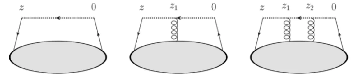
Figure 1. The first three “generic” diagrams for an insertion of the operator Q(z) in eq. (1.1).

Wilson lines are indicated as dotted.

so that any Green function in QCD with the insertion of the non-local operator in eq. (1.1) can equivalently be obtained from the correlation function of two local “heavy-light” op- erators. E.g. for quarks,

S

_h⁽⁰⁾

(vz)h0|T

{O(z) Φ(x₁

, . . . , x

n

)}|0i =

h0|T{

qh ¯

v

(zv)Γ ¯ h

v

q

(0) Φ(x

1

, . . . , x

n

)}|0i , (2.4) where Φ(x

1

, . . . , x

n

) stands for an arbitrary set of QCD fields at positions x

1

, . . . , x

n

, and similarly for gluons. With our choice v

₀

> 0 and for z > 0, the path ordering in the operator on the l.h.s. of eq. (2.4) is consistent with time ordering. For z < 0, the expressions on the l.h.s. and r.h.s. of eq. (2.4) both vanish. It is instructive to verify the equivalence in eq. (2.4) diagrammatically at the few lowest orders in perturbation theory. For definiteness, consider quark operators. On the one hand, from the definition of the path-ordered exponential in eq. (1.3), one obtains

Q

(z) = ¯ q(zv)Γ

1 + ig

Z z

0

dz

1

A

v

(z

1

v) + (ig)

² Z z

0

dz

1

Z z1

0

dz

2

A

v

(z

1

v)A

v

(z

2

v) +

· · ·

q(0) , (2.5) where we have used the shorthand notation A

v

= v

^µ

A

µ

. Notice that the factor 1/2! that naively appears in the third term of the expansion of the exponential function is replaced by the ordering of the integration regions. On the other hand, one can easily write the corresponding expression using the Feynman rules of the effective theory in eq. (2.1),

T

(¯ qh

_v

) (zv) Γ ¯ h

_v

q

(0) = 1

|v|

θ(z)δ

^(D−1)

(0

_⊥

)¯ q(zv)Γ

1 + ig

Z ∞

0

dz

₁

θ(z

−

z

₁

)A

_v

(z

₁

v) + (ig)

²

Z ∞

0

dz

2

Z ∞

0

dz

1

θ(z

−

z

1−

z

2

)A

v

(z

1

v + z

2

v)A

v

(z

2

v) + . . .

q(0) . (2.6) In this way, the 1/2! factor in the last term is compensated by a different mechanism:

there are two equivalent ways to couple the four h

v

fields in the Lagrangian insertions (ig)

²

/2! ¯ h

_v

A

^a_v

T

_a

h

_v2

with those in the currents ¯ qh

_v

(zv) and ¯ h

_v

q(0). Notice that discon- nected diagrams are not counted. The two expressions in eqs. (2.5) and (2.6) are obviously equal up to an overall factor, which is nothing but the free propagator of the “heavy”

field, S

_h⁽⁰⁾

(zv).

JHEP07(2020)161

3 Calculation

3.1 Generalities

We define the renormalization factors for generic composite operators O as

O(z) = Z

_O

O

B

, (3.1)

where O

_B

is the corresponding bare operator and the bare fields are related to the renor- malized ones as

A

^a,_µ^B

=

p

Z

₃

A

^a_µ

, q

B

=

p

Z

₂

q , h

^B_v

=

p

Z

_h

h

_v

. (3.2)

The bare QCD coupling constant g

B

is expressed as

g

B

= Z

_g

µ

g , (3.3)

where µ is the ’t Hooft mass and = (4

−

D)/2, with D being the running space-time dimension within the method of dimensional regularization [40–42]. Within the modified minimal-subtraction (MS) scheme, every RC is independent of dimensional parameters (masses and momenta) and can be represented as

Z(a) = 1 +

∞

X

n=1

z

⁽ⁿ⁾

(a)

ⁿ

, (3.4)

where a = g

²

/(16π

²

). Given a RC Z (a), the corresponding AD is defined as γ(a) =

±µ²

d ln Z(a)

dµ

²

=

± −a

∂z

⁽¹⁾

(a)

∂a

!

=

∞

X

n=1

(γ)

_n

a

ⁿ

. (3.5) Here, the sign depends on the way how the considered bare quantity, O

B

, is related to its renormalized counterpart, O. With our convention (3.1), the renormalization group (RG) equation for O assumes the form

µ

²

dO

dµ

²

= γ

O

O with γ

O

= µ

²

d ln Z

O

(a)

dµ

²

. (3.6)

Traditionally, in renormalizing coupling constants, wave functions and masses, the defining relation (3.1) is written with Z

O

on the left-hand side, e.g.,

Z

_m

m = m

_B

.

As a result, the ADs γ

₂

and γ

_h

, and the β function (see below) are defined with the minus sign version of eq. (3.5), but the ADs of composite operators (see below) with the plus sign. Customarily, one also defines Z

a

= Z

_g²

and refers to the corresponding AD as the QCD β function,

β(a) = a ∂z

⁽¹⁾_a

(a)

∂a =

∞

X

n=1

β

_n

a

ⁿ

. (3.7)

JHEP07(2020)161

The RCs Z

₂

and Z

_a

serve to renormalize the standard QCD Lagrangian and have been well known through three loops for a long time [43–45]. The RC Z

h

is known to the same accuracy for the time-like case v

²

> 0 [13] and will be used by us as convenient reference point. For the reader’s convenience, we quote the RCs as well as the corresponding ADs in appendices

B

and

A, respectively. Due to an overall

δ

^(D−1)

(x

⊥

) factor in position space, the self-energy and hence also the propagator of the “heavy” field h

_v

can only depend on the projection of its momentum onto v

^µ

, for which we use the notation

ω = p

·

v . (3.8)

The heavy-field self-energy is defined, as usual, as the sum of one-particle-irreducible am- putated diagrams,

ω Σ

h

(ω) = i

Z

d

^D

x e

^ip·xh0|T{h_v

(x) ¯ h

v

(0)}|0i

1PI, amputated

, (3.9) and the full propagator is then given by

S ˜

h

(ω) =

S ˜

_h⁰

(ω)

1 + Σ

_h

(ω) , S ˜

_h⁰

(ω) = 1

−ω−

i0 . (3.10)

Notice that the full propagator and the self-energy in Landau gauge satisfy the RG equa- tions,

µ

²

∂

∂µ

²

+ β(a) a ∂

∂a

S ˜

_h

= γ

_h

S ˜

_h

, (3.11)

µ

²

∂

∂µ

²

+ β(a) a ∂

∂a

Σ

h

=

−γ_h

Σ

h

. (3.12)

The renormalization factors Z

_Q

of the “heavy-light” operators in eq. (3.13) are calcu- lated from the corresponding vertex functions Γ(p, ω) as explained, e.g., in ref. [46]; the general formalism is the same for v

²

> 0 and v

²

< 0.

3.2 Renormalization constants and VEVs of qPDF operators

Let us first consider quark operators. Let

Q

i

(x) = ¯ q

i

(x)h

v

(x) , (3.13) where i is the spinor index, which we do not show in what follows. One can show that this operator is multiplicatively renormalized. The corresponding RC Z

Q

,

Q(x) = Z

_Q

Q

B

(x) , (3.14)

was calculated to three-loop accuracy for the time-like case v

²

> 0 [13] and is the same for space-like v

²

< 0. The RC Z

_Q

of the non-local operator defined in eq. (1.1) is related to Z

Q

as [27]

Q(z) =

Z

_QQB

(z) , Z

_Q

= Z

_Q²

. (3.15)

JHEP07(2020)161

The corresponding ADs are obviously related as

γ

_Q

(z) = 2 γ

Q

. (3.16)

The equality (3.15) implies that Z

_Q

does not depend on the Dirac structure Γ in the definition of the operator

Q(z), eq. (1.1). We have checked this relation at the two-loop

level by explicit calculation of the VEV of

Q

(z) to three-loop accuracy; see section

5. This

VEV is non-vanishing in perturbation theory only for the Dirac structure Γ = γ

_µ

, in which case it follows from Lorentz invariance that

h0|Qµ|0i ∝

v

µ

. Thus, it is sufficient to consider Π(z) =

h0|v^µQµ

(z)|0i =

h0|¯

q(zv)/ v[zv, 0]q(0)|0i , (3.17) or, equivalently, the momentum space correlation function,

Π(ω) =

e

i

Z

d

^D

x e

^ip·xh0|T{Q(x)/

vQ

^†

(0)}i , (3.18) where the current Q(x) is defined in eq. (3.13). It is easy to see that

Π(z > 0) = 1 i

Z

d

^D−1

x

⊥

Z

d

^D

p

(2π)

^D

e

^−ip·x

Π(p) ˜ with z =

±x·

v , (3.19) where the

±

sign corresponds to the choice v

²

=

±1. Notice that Π(z >

0) does not depend on the “contact” terms in ˜ Π(p) of the form

const ·

ω

²

, which suffer from an extra UV divergence coming from the integration region around x = 0 in eq. (3.18). Thus, in momentum space, it is natural to consider instead of ˜ Π(p) an analog of the Adler function, namely

D(ω) = ˜ ω d dω

π

²

ω

²

Π(ω) ˜

. (3.20)

The corresponding RG equation for D(ω) reads

µ

²

∂

∂µ

²

+ β(a) a ∂

∂a

D ˜ = 2γ

_Q

D. ˜ (3.21)

The gluon case is more involved because, in the presence of the external four-vector v

^µ

, the components parallel and transverse to v

^µ

can be renormalized differently. Introducing the corresponding projection operators,

g

_µν^k

= v

µ

v

ν

v

²

, g

_µν^⊥

= g

µν−

v

µ

v

ν

v

²

, (3.22)

we can define two multiplicatively renormalizable gauge-invariant local operators in effec- tive theory with adjoint “heavy” scalars as

²

G

^k⊥_µν

(x) =

h

g

_µα^k

g

^⊥_νβ−

g

^k_να

g

^⊥_µβ i

gF

^αβ

(x)h

v

(x) ,

G

^⊥⊥_µν

(x) = g

_µα^⊥

g

^⊥_νβ

gF

^αβ

(x)h

_v

(x) , (3.23)

2Notice that we include the QCD coupling g in the definition of the operators, which simplifies the renormalization factors.

JHEP07(2020)161

with the RCs Z

_k⊥

and Z

⊥⊥

,

G

^k⊥_µν

= Z

k⊥

G

^k⊥_µν

B

, G

^⊥⊥_µν

= Z

⊥⊥

G

^⊥⊥_µν

B

. (3.24)

We will denote the corresponding ADs as γ

_k⊥

and γ

⊥⊥

respectively. The correlation func- tions of these operators have the form

h0|G^⊥⊥_µν

(x) ¯ G

^⊥⊥_αβ

(0)|0i = (g

_µα^⊥

g

^⊥_νβ−

g

_να^⊥

g

^⊥_µβ

)Π

⊥⊥

(x) ,

h0|G^k⊥_µν

(x) ¯ G

^k⊥_αβ

(0)|0i = (g

_µα^k

g

^⊥_νβ−

g

_να^k

g

^⊥_µβ−

g

^k_µβ

g

^⊥_να

+ g

_νβ^k

g

^⊥_µα

)Π

k⊥

(x) ,

h0|G^⊥⊥_µν

(x) ¯ G

^k⊥_αβ

(0)|0i = 0 , (3.25)

where ¯ G

^⊥⊥_αβ

= g

_µα^⊥

g

_νβ^⊥

gF

^αβ

¯ h

_v

, etc., and are renormalized by squares of the corresponding RCs in eq. (3.24). In this notation, a generic two-gluon vacuum correlation function related to the qPDF operator in eq. (1.2) takes the form

Π

_µναβ

(x) =

h0|g²

F

_µν

(x)h

_v

(x)¯ h

_v

(0)F

_αβ

(0)|0i

= (g

^⊥_µα

g

_νβ^⊥ −

g

_να^⊥

g

_µβ^⊥

)Π

_⊥⊥

(x) + (g

^k_µα

g

^⊥_νβ−

g

_να^k

g

_µβ^⊥ −

g

^k_µβ

g

^⊥_να

+ g

^k_νβ

g

^⊥_µα

)Π

_k⊥

(x)

= (g

µα

g

νβ−

g

να

g

µβ

) Π

⊥⊥

(x) + 1

v

²

(v

_µ

v

_α

g

_νβ−

v

_ν

v

_α

g

_µβ−

v

_µ

v

_β

g

_να

+ v

_ν

v

_β

g

_µα

) [Π

_k⊥

(x)

−

Π

⊥⊥

(x)] . (3.26) For future reference, we introduce the corresponding “Adler” functions:

D ˜

⊥⊥

(ω) = ω d dω

Π ˜

⊥⊥

(ω) ω

³

!

,

D ˜

_k⊥

(ω) = ω d dω

Π ˜

k⊥

(ω) ω

³

!

, (3.27)

where

D

e⊥⊥

(ω) = i

Z

d

^D

x e

^ip·x

Π

⊥⊥

(x), D

ek⊥

(ω) = i

Z

d

^D

x e

^ip·x

Π

k⊥

(x) . (3.28) The functions ˜ D

⊥⊥

(ω) and ˜ D

_k⊥

(ω) satisfy the standard RG equations like eq. (3.21) with the ADs (2 γ

⊥⊥

) and (2 γ

k⊥

) respectively. In the qPDF literature, following refs. [37,

38],

one usually introduces a different operator basis,

J

₁^µν

= g F

^µν

h

_v

, J

₂^µν

= v

_ρ

v

²

g (F

_a^µρ

v

^ν−

F

_a^νρ

v

^µ

) h

^a_v

, (3.29) so that, obviously,

J

₂^µν

(x) = G

^k⊥_µν

(x) , J

₁^µν

(x) = G

^⊥⊥_µν

(x) + G

^k⊥_µν

(x) . (3.30) The operators J

1

and J

2

are renormalized by a triangular 2

×

2 mixing matrix Z

ik

such that Z

₂₁

= 0 and Z

₁₂−

Z

₂₂

+ Z

₁₁

= 0 to all orders. These relations imply that

Z

₁₁

= Z

⊥⊥

, Z

₂₂

= Z

_k⊥

. (3.31)

Notice that we ignore mixing with gauge-noninvariant operators as they do not contribute

to gauge-invariant observables. With the main definitions at hand, we proceed to describe

the calculation procedure.

JHEP07(2020)161

3.3 Reduction

The generation of the Feynman diagrams and their reduction to master integrals (MIs) have been done in the standard way, using the programs QGRAF [47] and FIRE6 [48], respectively.

³

The reduction typically results in a sum of MIs with coefficients being rational functions of the space-time dimension D. In addition, every MI is multiplied by a factor of the form

(v

²

)

ⁿ¹

ω

ⁿ²

, (3.32)

and color factors like C

F

, C

A

, etc. We have checked that our results for the time-like case v

²

= 1 are in full agreement with ref. [13]. In our calculation, we have used the values of the relevant MIs given in ref. [13].

3.4 Master integrals: time-like versus space-like

The MIs for v

²

> 0, which we refer to as time-like, are analytic functions of ω. They are real for ω < 0 and have a branch cut at ω > 0. On dimensional grounds, each MI has the form

M (ω < 0, v

²

= 1;

n) = (−2ω)^dM

M (;

n)

, d

^M

= D L

−

2

X

l

n

_l−X

h

n

_h

, (3.33) where M (;

n) is a real function of the space-time dimension

D, d

^M

is the dimension of the MI M , L stands for the number of loops and the sums over l and h count the indices n

l

and n

h

of all usual QCD (“light”) and special (“heavy”) lines of the integral. The argument

n

stands for the collection of all indices. We assume that every MI is of scalar type, so that the corresponding integrand is given by a product of denominators involving

“light” (massless) and “heavy” propagators, possibly raised to certain (integer) powers (indices). The reduction to scalar MIs is certainly possible at the three-loop level; see, e.g., refs. [13,

51]. The restriction to the normalization

v

²

= 1 can easily be relaxed. Indeed, the

“heavy” propagator in eq. (2.2) is a homogeneous function w.r.t. the rescaling v

^µ→

λv

^µ

. Thus, we have M (λω, λ

²

v

²

;

n) =

λ

^−dMv

M(ω, v

²

;

n), where

d

^M_v

=

−P

h

n

_h

stands for the v dimension of the integral, so that, for generic time-like v

²

> 0, we have

M (ω < 0, v

²

> 0;

n) = (−2ω)^dM

(v

²

)

^{(−dM+dMv )/2}

M(;

n)

= (−2ω)

^dMv

4ω

²

v

²

(d^M−d^M_v )/2

M (;

n)

. (3.34) The result for ω > 0 is obtained by analytic continuation. In this way, the MI acquires an imaginary part according to the usual causal prescription ω

→

ω + i0, so that 4ω

² →

(−2ω

−

i0)

²

. In order to calculate a MI for the space-like case v

²

< 0, it is useful to start from the so-called α representation of the time-like MI,

⁴

M(ω, v

²

> 0;

n) =

Γ (Σn

−

Ld/2)

Q

α

Γ (n

α

)

Z

Y

α

dz

α

z

_α^nα−1

δ (1

−

Σz) (F

−

i0)

^Ld/2−Σn

U

(L+1)d/2−Σn

, (3.35)

3We have also used the Mathematica program LiteRed 1.4 [49,50] and the REDUCE package Grinder [51]

for testing purposes and the identification of the MIs.

4Within HQET, this was considered in ref. [52]. A general discussion can be found, e.g., in refs. [50,53].

JHEP07(2020)161

where Σn =

P

α

n

_α ≡P

l

n

_l

+

P

h

n

_h

, Σz =

P

α

z

_α

, and U and F are homogeneous poly- nomials of degree L and L + 1 in the integration parameters z

α

, respectively. The function U does not depend on kinematic invariants, whereas the function F can be written as

F =

−2

ω T

p

+ v

²

T

v

, (3.36)

with polynomials T

_p

and T

_v

that only depend on the parameters z

_α

and are defined to be positive in the integration region of eq. (3.35). Notice that, in eq. (3.35), we do not assume that ω < 0, so that, for v

²

> 0, the MI acquires an imaginary part at ω > 0 according to the Feynman prescription F

7→

F

−

i0. The crucial observation is that, if one

simultaneously

changes the signs of v

²

and ω, the MI receives an overall phase factor,

M (ω > 0, v

²

< 0;

n) =

e

−iπ(Ld/2−Σn)

M(−ω,

|v²|;n)

= e

^iπL

(−1)

^Σn

M (−ω,

|v²|;n)

, (3.37) as, by definition,

(F

−

i0)

^λ

:=

(

F

^λ

if F > 0 ,

(−F )

^λ

e

^−iπλ

if F < 0 . (3.38) Thus, we obtain

M (ω > 0, v

²

< 0;

n) =

e

^iπL

(−1)

^Σn|2ω|^dM|v²|^{(−dM+dMv )/2}

M(;

n)

= e

^iπL

(−1)

^{(dM0 +dMv )/2}|2ω|^dM|v²|^{(−dM+dMv )/2}

M(;

n)

= (−2ω)

^dMv

4ω

²

v

² −

i0

(d^M−d^M_v )/2

M (;

n)

, (3.39)

where d

^M₀

= d

^M|₌₀

. A generic Green function G(ω, v

²

) with mass dimension d

^G

and v di- mension d

^G_v

is given by the sum of MIs multiplied by extra kinematic factors (v

²

)

^j1

(−2ω)

^j2

, where j

1

and j

2

are integers that satisfy the obvious relations

j

₂

+ d

^M

= d

^G

, 2j

₁

+ j

₂

+ d

^M_v

= d

^G_v

. (3.40) It is easy to see that

(v

²

)

^j1

(−2ω)

^j2

M(ω < 0, v

²

> 0;

n) = (−2ω)^dGv

4ω

²

v

²

(d^G−d^G_v)/2

M (;

n)

, (v

²

)

^j1

(−2ω)

^j2

M(ω > 0, v

²

< 0;

n) = (−2ω)^dGv

4ω

²

v

² −

i0

(d^G−d^G_v)/2

M (;

n)

, (3.41) so that, upon this multiplication, the mass and v dimensions of a particular MI are substi- tuted by those of the Green function in question and are the same for the contributions of all MIs and for all Feynman diagrams. As a consequence, going over from v

²

> 0, ω < 0 to v

²

< 0, ω > 0, the Green function acquires an overall phase factor,

G(ω > 0, v

²

< 0) = e

^{iπ(dG+dGv)/2}

G(−ω,

|v²|)

= e

^iπL

(−1)

^(dG0+dGv)/2

G(−ω,

|v²|)

, (3.42)

JHEP07(2020)161

where d

^G₀

= d

^G|₌₀

, which is the final result. Thus, we conclude the following:

•

A generic Green function at v

²

< 0 can be obtained from the result at v

²

> 0 by the (possible) global sign change (−1)

^(dG0+dGv)/2

, which is the same to all orders of perturbation theory, and the formal substitution

(−2ω)

^dG0

ln(−2ω

−

i0)|

_v2=1 →

(2ω)

^dG0 h

ln(2ω + i0)

−

i π 2

i

v²=−1

, (3.43) where we assume

|v²|

= 1 and the Feynman causal prescription.

•

Since, in minimal schemes, the RCs and ADs neither depend on the global sign nor on the value of the external momentum, they are not affected by the analytic continuation in v

²

and are the same for time-like (v

²

= 1) and space-like (v

²

=

−1)

kinematics.

4 Transition to position space

Without loss of generality, we may assume v

^µ

= (1, 0, 0, 0) and v

^µ

= (0, 0, 0, 1) for the time- like and space-like cases, respectively. For this choice, the variable ω is the energy, ω = p

0

, for the time-like case and the z component of the momentum up to a minus sign, ω =

−p_z

, for the space-like case. The relation between generic correlation functions established in the previous section, therefore, connects a v

²

= 1 Green function for negative energy with the corresponding v

²

=

−1 Green function with negative momentum in

z direction. The corresponding position-space variables for these cases are obviously the separation in time t and distance z of the quark and the antiquark in the operator in eq. (1.1). In the time-like case, the transition is performed with the help of the generic formula

Z

dω

2π e

^{−it ω}

(−2ω

−

i0)

^−2L−n

= e

^i(2L+n)π/2

2 Γ(n + 2 L ) θ(t) t 2

2L+n−1

= i

2 Γ(n + 2 L ) θ(t) i t 2

2L+n−1

, (4.1)

where we assume n to be integer.

Thus, renormalized time dependent correlation functions are expressed in terms of the following combination

ln i t e

^γE

2

≡

ln t

2 + γ

_E

+ i π

2 , (4.2)

where Euler’s constant γ

E

appears naturally due to a universal factor,

Γ(n + 2 L )

≡

Γ(1 + 2 L ) (1 + 2L)

_(n−1)

, (4.3) with (1 + 2L)

_(n−1)

being the Pochhammer symbol. There is no γ

E

in momentum space results. The analogue of eq. (4.1) for the space-like case is

Z

dp

_z

2π e

^{iz pz}

(−2p

_z

+ i0)

^−2L−n

= e

−i(2L+n)π/2

2 Γ(n + 2 L ) z

2

2L+n−1

=

−i

2 Γ(n + 2 L )

−i z

2

2L+n−1

. (4.4)

JHEP07(2020)161

Comparing eqs. (4.1) and (4.4), we infer that the transition from a time-like to a space-like renormalized correlation function in position space amounts to the formal substitution

ln it

2

→

ln z

2 , (4.5)

up to a possible change of the global sign.

5 Results

In this section, we collect our results for the case of standard QCD with the SU(3) gauge group and n

f

active quarks triplets. Notice that the results for the self-energy and the propagator of the “heavy” field, the ADs γ

₂

and γ

_h

as well as the corresponding RCs are gauge dependent. The expressions below are given in Landau gauge, as it is most relevant for lattice applications. Full results for a generic gauge group and including the gauge as well as the momentum/position dependence are appended in the arxiv submission of this paper as auxiliary files in computer readable format. Many results given in the text and in the auxiliary files have originally been obtained by other authors and have been included here for completeness. In particular the AD of the heavy-light current γ

_Q

was computed at one, two and three loops in refs. [54,

55], refs. [12,56] and ref. [13], respectively. The AD

γ

h

of the “heavy” field h

v

was computed at two and three loops in ref. [12] and refs. [13,

57],

respectively, and, recently, at four loops in refs. [58,

59]. The RCs

Z

₃

, Z

₂

and Z

_a

have been known through three loops for a long time [43–45]. The VEV Π in eq. (1.1) was computed at two loops in ref. [60] and at three loops in ref. [61]. Notice that all these results for the ADs γ

_h

, γ

_Q

and for the VEV Π were obtained for the time-like choice of the vector v

^µ

, with v

²

= 1. Our contribution is to clarify the changes for the space-time choice v

²

=

−1.

We have also computed the VEV of the gluon off-light-cone operator in eq. (1.2) in the three-loop approximation as well the corresponding anomalous dimensions at two loops.

Our results are in agreement with the two-loop VEV found in ref. [62] and the one-loop ADs first computed in refs. [37,

38].

5.1 Anomalous dimensions and renormalization constants

As follows from eq. (3.4), ADs and RCs are not sensitive to the sign choice of v

²

. The analytic results for the ADs β, γ

_Q

, γ

_h

, γ

₂

, γ

⊥⊥

and γ

_k⊥

are listed in appendix

A, and those

for the RCs Z

a

, Z

Q

, Z

h

, Z

2

, Z

⊥⊥

and Z

k⊥

in appendix

B.

5.2 Correlation functions: momentum space

Our result for the self-energy of the “heavy” field, Σ

h

, defined in eq. (3.9) for the space-like case v

²

=

−1 can be written as⁵

Σ

_h

(µ = 2ω, v

²

=

−1) = Σ^t_h

+ (δΣ

^s_h

)

^Re

+ (δΣ

^s_h

)

^Im

=

3

X

n=1

(Σ

^t_h

)

n

a

ⁿ

+

3

X

n=1

(δΣ

^s_h

)

^Re_n

a

ⁿ

+ i

3

X

n=1

(δΣ

^s_h

)

^Im_n

a

ⁿ

, (5.1)

5In what follows, we do not show the trivial dependence of the self-energy Σh(p) and the corresponding propagatorShon color indices. Furthermore, in eq. (5.13), we do not display the factorδ^(D−1)(x⊥).

JHEP07(2020)161

where the first term corresponds to the time-like self-energy,

Σ

_h

(µ =

−2ω, v²

= 1) = Σ

^t_h

=

3

X

n=1

(Σ

^t_h

)

n

a

ⁿ

, (5.2)

and the addenda δΣ

^s_h

arise when going over to the space-like case using the substitution rule in eq. (3.43),

ln

ⁿ

(−2ω)

→

ln

ⁿ

(2ω) +

j≤[n/2]

X

j=1

−π²

4

j

n 2j

ln

^n−2j

(2ω)

−

i

j≤[(n−1)/2]

X

j=0

π 2

−π²

4

j

n 2j + 1

ln

^n−2j−1

(2ω) . (5.3)

Using Landau gauge, we find the following expressions:

(Σ

_h^t

)

₁

=

−

16

3 , (Σ

_h^t

)

₂

=

−

4355

18

−12π²

+ n

_f

152

9 + 8 9 π

²

,

(Σ

_h^t

)

₃

=

−

3741889

324

−

8765

9 π

²

+ 4603

360 π

⁴

+ 893ζ

₃

+ 44π

²

ζ

₃−

372ζ

₅

+n

_f

388024

243 + 3316

27 π

²−

104

135 π

⁴−120ζ₃

+ n

²_f

−

31232 729

−

256

81 π

²

+ 160 27 ζ

₃

,

(δΣ

hs

)

^Re₁

= 0, (δΣ

hs

)

^Re₂

= 14π

²−

4 3 π

²

n

f

, (δΣ

_h^s

)

^Re₃

= 2873

3 π

²−

1322

9 π

²

n

_f

+ 128 27 π

²

n

²_f

, (δΣ

_h^s

)

^Im₁

=

−4π ,

(δΣ

_h^s

)

^Im₂

=

−97π

+ 64

9 π n

_f

, (δΣ

_h^s

)

^Im₃

=

−

188723

36 π

−132π³−

8

5 π

⁵−

369

2 πζ

₃

+ n

_f

20236

27 π + 160

9 π

³

+ 160 3 πζ

₃

+n

²_f

−

1744 81 π

−

16

27 π

³

. (5.4)

Notice that the full dependence on ln[µ/(2ω)] in eq. (5.4) can be easily restored from the evolution eq. (3.12) with the use of the AD γ

_h

as given in appendix A.

Assuming n

_f

= 3 and substituting a

s

= 4a

≡

α

s

/π, we get numerically:

(Σ

_h^t

)

_nf=3

=

−1.33333

a

_s−

17.7121 a

²_s−

180.297 a

³_s

, (δΣ

_h^s

)

^Re_nf=3

= 6.1685 a

²_s

+ 86.3076 a

³_s

,

(δΣ

hs

)

^Im_nf=3

=

−3.14159

a

s−

14.8571 a

²_s−

206.265 a

³_s

. (5.5)

Notice that the heavy-field self-energy at v

²

=

−1 acquires a large imaginary part, whereas

the difference in the real part is minor.

JHEP07(2020)161

Next, we consider the momentum-space correlation function in eq. (3.18). Our result for ˜ D reads

⁶

π

²

D(µ ˜ = 2ω, v

²

=

−1) =−

D ˜

^t

+ (δ D ˜

^s

)

^Re

+ (δ D ˜

^s

)

^Im

=

−

2

X

n=0

( ˜ D

^t

)

n

a

ⁿ

+

2

X

n=0

(δ D ˜

^s

)

^Re_n

a

ⁿ

+ i

2

X

n=0

(δ D ˜

^s

)

^Im_n

a

ⁿ

, (5.6) where, as above, the first term corresponds to the time-like correlation function,

π

²

D(µ ˜ =

−2ω, v²

= 1) = ˜ D

^t

=

2

X

n=0

( ˜ D

^t

)

n

a

ⁿ

. (5.7)

The coefficients in eq. (5.6) are given by

( ˜ D

^t

)

0

= 3 , ( ˜ D

^t

)

1

= 68 + 16 3 π

²

, ( ˜ D

^t

)

2

= 24749

6 + 3680

9 π

²−

32

27 π

⁴−

3872

3 ζ

3

+ n

_f

−

1849 9

−

328

27 π

²

+ 64ζ

3

,

(δ D ˜

^s

)

^Re₀

= 0 , (δ D ˜

^s

)

^Re₁

= 0 , (δ D ˜

^s

)

^Re₂

= 90π

²−

4π

²

n

_f

,

(δ D ˜

^s

)

^Im₀

= 0 , (δ D ˜

^s

)

^Im₁

=

−12π ,

(δ D ˜

^s

)

^Im₂

=

−

3314

3 π

−

776

9 π

³

+ n

_f

52π + 32 9 π

³

. (5.8)

For n

f

= 3, we have numerically

(δ D ˜

^t

)

_nf=3

= 3. + 30.1595 a

_s

+ 359.267 a

²_s

, (δ D ˜

^s

)

^Re_nf=3

= 48.1143 a

²_s

,

(δ D ˜

^s

)

^Im_nf=3

=

−9.42478

a

s−

332.689 a

²_s

. (5.9) Finally, we present below our results for the two momentum-space correlators,

D ˜

⊥⊥

(µ = 2ω, v

²

=

−1) =

a

D ˜

^t_⊥⊥

+ (δ D ˜

^s_⊥⊥

)

^Re

+ (δ D ˜

_⊥⊥^s

)

^Im

= a

X²

n=0

( ˜ D

_⊥⊥^t

)

_n

a

ⁿ

+

3

X

n=0

(δ D ˜

_⊥⊥^s

)

^Re_n

a

ⁿ

+ i

2

X

n=0

(δ D ˜

_⊥⊥^s

)

^Im_n

a

ⁿ

,

D ˜

_k⊥

(µ = 2ω, v

²

=

−1) =

a

D ˜

^t_k⊥

+ (δ D ˜

^s_k⊥

)

^Re

+ (δ D ˜

_k⊥^s

)

^Im

= a

X²

n=0

( ˜ D

_k⊥^t

)

_n

a

ⁿ

+

3

X

n=0

(δ D ˜

^s_k⊥

)

^Re_n

a

ⁿ

+ i

2

X

n=0

(δ D ˜

_k⊥^s

)

^Im_n

a

ⁿ

, (5.10)

6Notice that there is an overall minus sign between the time-like and space-like correlation functions, unlike for the self-energy Σh.