Transverse momentum dependent parton quasidistributions Xiangdong Ji,

(1)

Transverse momentum dependent parton quasidistributions

Xiangdong Ji,

^1,2

Lu-Chang Jin,

^3,4

Feng Yuan,

⁵

Jian-Hui Zhang,

⁶

and Yong Zhao

⁷

1

Tsung-Dao Lee Institute, and College of Physics and Astronomy, Shanghai Jiao Tong University, Shanghai 200240, China

2

Maryland Center for Fundamental Physics, Department of Physics, University of Maryland, College Park, Maryland 20742, USA

3

Department of Physics, University of Connecticut, Storrs, Connecticut 06269, USA

4

RIKEN-BNL Research Center, Brookhaven National Laboratory, Building 510, Upton, New York 11973, USA

5

Nuclear Science Division, Lawrence Berkeley National Laboratory, Berkeley, California 94720, USA

6

Institut für Theoretische Physik, Universität Regensburg, D-93040 Regensburg, Germany

7

Center for Theoretical Physics, Massachusetts Institute of Technology, Cambridge, Massachusetts 02139, USA

(Received 7 December 2018; published 6 June 2019)

We investigate the transverse momentum dependent parton distributions (TMDs) in the parton quasidistributions framework. The longstanding hurdle of the so-called pinch pole singularity from the spacelike gauge links in the TMD definitions can be resolved by the finite length of the gauge link along the hadron moving direction. In addition, with the soft factor subtraction, the quasi-TMD is free of linear divergence. We further demonstrate that the energy evolution equation of the quasi-TMD a.k.a. the Collins- Soper evolution, only depends on the hadron momentum. This leads to a clear matching between the quasi- TMD and the standard TMDs.

DOI: 10.1103/PhysRevD.99.114006

I. INTRODUCTION

Transverse momentum dependent parton distributions (TMDs) are one of the major focuses in nucleon tomography studies at existing and future facilities [1]. Theoretically, they have attracted great interest starting in the early 1980s, and considerable developments have been achieved in recent years [2 – 5]. Pioneering work to compute the TMD matrix elements from lattice QCD has also been performed in Ref. [6], where the longitudinal momentum fraction x for the quarks has been integrated out. Such results have generated interest in computing TMDs from lattice QCD in the hadron physics community.

In the last few years, there has been great progress on computing parton physics from lattice QCD, thanks to the large momentum effective theory (LaMET) [7]. LaMET is based on the observation that parton physics defined in terms of lightcone correlations can be obtained from time- independent Euclidean correlations, now known as quasi- distributions, boosted to the infinite momentum frame. For a finite but large momentum feasible on the lattice, the two

quantities are not identical, but they can be connected to each other by a perturbative matching relation, up to power corrections that are suppressed by the hadron momentum.

LaMET has been applied to computing various PDFs [8 – 14] as well as meson DAs [15,16] (see also [17,18]

for slightly different proposals). In addition, theoretical developments have been achieved on the renormalization of the parton quasidistributions functions and on their matching to the usual PDFs [12,19 – 40]. Unfortunately, there has been no lattice effort to compute the TMDs from the quasi-TMDs (Q-TMDs). The major hurdle is that the formulation of the TMDs is different from the integrated PDFs and, in particular, the gauge links associated with the Q-TMDs lead to the so-called pinch pole singularities. This is a generic feature of the TMDs defined with a space-like gauge link [2,5]. We have to either subtract or regulate these singularities before we can make meaningful computations of the Q-TMDs on the lattice [3]. In Ref. [41], a soft factor subtraction involving transverse gauge links has been proposed to formulate the Q-TMDs. However, this formal- ism may have practical difficulties for lattice computations at present.

In this paper, we will reinvestigate the TMDs in the LaMET or Q-TMDs framework. We will show that, with finite length gauge links in the Q-TMDs, there will be no pinch pole singularity. This will pave the way to perform the TMD calculations on the lattice. Moreover, with an Published by the American Physical Society under the terms of

the Creative Commons Attribution 4.0 International license.

Further distribution of this work must maintain attribution to

the author(s) and the published article ’ s title, journal citation,

and DOI. Funded by SCOAP

³

.

(2)

explicit one-loop calculation, we demonstrate that the energy evolution of the TMDs depends on the hadron momentum. This will clarify an important issue to match the Q-TMDs to the standard TMDs extracted from the experiments.

Our focus will be on the basics of the formalism and setting up the foundation for future numerical simulations on the lattice. Let us start with the unsubtracted Q-TMD quark distribution defined with finite length gauge links,

q ð x _z ; k ⃗

_⊥

; L Þj

^ðunsubÞ

¼ 1 2

Z dzd

²

b ⃗

_⊥

ð2πÞ

³

e

^−ik^z

^z−i

^⃗

^k

^⊥^·^⃗

^b

^⊥

h PS j ψ ¯

− b ⃗

_⊥

2 ; − z

2 × L

^†

n

zð−^⃗b^⊥₂

;−

₂^z;−^⃗b₂^⊥

;LÞ γ ^z L

^†

Tð−

^⃗b₂^⊥

;L;

^⃗b^⊥₂

;LÞ L

n

zð^⃗b₂^⊥

;

^z₂;^⃗b₂^⊥

;LÞ

× ψ b ⃗

_⊥

2 ; z 2

j PS i ; ð 1 Þ

where ð b ⃗

_⊥

; z Þ represents the 3-dimensional coordinate space variable separated by the quark and antiquark fields, x _z ¼ k _z =P _z and the proton is moving along þˆ z direction,

⃗ k

_⊥

represents the transverse momentum of the quark. In the above definition, L n

_zð⃗y_⊥

;z

₁;⃗y_⊥

;z

₂Þ

¼ P exp ½− ig R _z

z

₂1

d λ n _z · A ðλ n _z þ y ⃗

_⊥

Þ represents the gauge link along the z ˆ direc- tion with the large length L ≫ j z j , where the 4-vector n _z is defined as n

^μ

z ¼ ð0 ; 0 ; 0 ; 1Þ . We have also included a transverse gauge link to make the gauge links connected as shown in Fig. 1(a).

In the TMD formalism, it has been demonstrated that the soft factor subtraction plays an important role to properly address the relevant factorization properties [3]. In this paper, we introduce the following soft factor subtraction,

q

^ð^sub^Þ

ðx z ; b ⃗

_⊥

Þ ¼ q

^ðunsubÞ

ffiffiffiffiffiffiffiffiffiffiffiffiffiffiffiffiffiffiffiffiffiffiffiffiffi ð x _z ; b ⃗

_⊥

; L Þ S ⁿ

^z

^;n

^z

ð b ⃗

_⊥

; L Þ

q ; ð2Þ

where q

^ðunsubÞ

ð x _z ; b ⃗

_⊥

; L Þ is the unsubtracted Q-TMD in Eq. (1) in the Fourier transform b ⃗

_⊥

-space with respect to the transverse momentum k ⃗

_⊥

, and S ⁿ

^z

^;n

^z

ð b ⃗

_⊥

; L Þ is defined as

S ⁿ

^z

^;n

^z

ð b ⃗

_⊥

; L Þ ¼ h0jL

^†

Tð

^b^⃗₂^⊥

;−L;−

^b^⃗₂^⊥

;−LÞ L

^†

n

_zð^b^⃗^⊥₂

;0;

^⃗b₂^⊥

;−LÞ L

^†

n

_zð^b^⃗₂^⊥

;L;

^⃗b₂^⊥

;0Þ

× L _Tð

^⃗b_⊥

2

;L;−

^b^⃗₂^⊥

;LÞ L

n

zð−^b^⃗^⊥₂

;L;−

^⃗b₂^⊥

;0Þ

× L

n

zð−^b^⃗₂^⊥

;0;−

^b^⃗₂^⊥

;−LÞ j0i ; ð 3 Þ

with L n

_z

being the longitudinal gauge link along the z ˆ direction and L T the transverse gauge link at z ¼ L and z ¼ − L, as shown in Fig. 1(b). In other words, the above soft factor is just a Wilson loop.

The rest of this paper is organized as follows. In Sec. II, we will show the absence of pinch pole singularity in the Q- TMD with finite length gauge links with an explicit calculation at one-loop order. In Sec. III, we will discuss the matching between the Q-TMD and the standard TMD.

We then summarize our paper in Sec. IV.

II. ABSENCE OF THE PINCH SINGULARITY IN Q-TMDS

To show that we do not encounter the pinch pole singularity, we will carry out a one-loop calculation. We take the example of quark Q-TMD on a quark target. In Feynman gauge, the one-loop diagrams are shown in Figs. 2 and 3. The final result can also serve as a matching between the Q-TMD and the standard TMD. Because of the finite length of the gauge links, the eikonal propagator in these diagrams will be modified accordingly,

ð− ig Þ in

^μ

n · k i ϵ ⇒ ð− ig Þ in

^μ

n · k ð1 − e

^in·kL

Þ ; ð 4 Þ

where n

^μ

represents the gauge link direction. In the present case n

^μ

¼ n

^μ

z . In perturbative calculations, we will make use of the large length limit j LP _z j ≫ 1 . By doing that, many of previous results can be applied to our calculations.

For example, in the large L limit, we have the following identity: lim _L→∞ _n·k

¹

e

^iLn·k

¼ i πδð n · k Þ .

At one-loop order, the pinch pole singularity could potentially come from the diagram (c) of Fig. 2 in the limit of infinite gauge link with L → ∞ ,

(a) (b)

FIG. 1. Illustration of the gauge links in the unsubtracted quasi-TMD (a) and the soft factor (b).

(3)

q

^ð1Þ

ð x _z ; k ⃗

_⊥

Þj ^L→∞

_2ðcÞ

¼ 1 2

Z dk

⁰

dk _z

ð2πÞ

⁴

uðpÞγ ¯ ^z ðigt ^a Þðigt ^a Þ − i n · ð P − k Þ − i ϵ

× i

n · ð P − k Þ þ i ϵ

−i

ð P − k Þ

²

u ð p Þδð k _z − x _z P _z Þ

¼ α s

4π

²

C _F P _z

ffiffiffiffiffiffiffiffiffiffiffiffiffiffiffiffiffiffiffiffiffiffiffiffiffiffiffiffiffiffiffiffiffiffi ð1 − x _z Þ

²

P

²

_z þ k ⃗

²_⊥

q 1

ð1 − x _z Þ P _z þ i ϵ

× 1

ð1 − x _z Þ P _z − i ϵ : ð 5 Þ

For the case of integrated parton distributions, we integrate over k ⃗

_⊥

to obtain the one-loop result. However, in the current case, we have to keep the transverse momentum ⃗ k

_⊥

. In addition, we note that the above contribution is power suppressed by k ⃗

_⊥

=P _z for x _z ≠ 1 . That means to leading power in P _z this diagram only contributes to δð1 − x _z Þ , and can be written as

q

^ð1Þ

ð x _z ; k ⃗

_⊥

Þj ^L→∞

_2ðcÞ

¼ α s

4π

²

C _F δð1 − x _z Þ

×

Z dk _z

ffiffiffiffiffiffiffiffiffiffiffiffiffiffiffiffi k

²

_z þ k ⃗

²_⊥

q 1

k _z þ i ϵ 1

k _z − i ϵ : ð 6 Þ

The above integral is not well-defined, because the two poles are pinched. We are forced to take the pole at k _z ¼ 0 , which is, however, divergent. This is a common issue for parton distributions defined with gauge links along the spacelike direction [2,5].

With finite length gauge links, the above result will be modified to

q

^ð1Þ

ð x _z ; k ⃗

_⊥

Þj

_2ð

c

Þ

¼ α s

4π

²

C _F P _z

ffiffiffiffiffiffiffiffiffiffiffiffiffiffiffiffiffiffiffiffiffiffiffiffiffiffiffiffiffiffiffiffiffiffi ð1 − x _z Þ

²

P

²

_z þ ⃗ k

²_⊥

q

× 1

ð1 − x _z Þ P _z 1 ð1 − x _z Þ P _z

× ð1 − e ⁱ

^ð1−

^x

^z^Þ

^P

^z

^L Þð1 − e

⁻

ⁱ

^ð1−

^x

^z^Þ

^P

^z

^L Þ ; ð 7 Þ where we have used Eq. (4). We find again that this result is power suppressed for x _z ≠ 1 . Therefore, we can simplify the above equation as

q

^ð1Þ

ð x _z ; k ⃗

_⊥

Þj

_2ðcÞ

¼ α s

4π

²

C _F δð1 − x _z Þ Z dk _z

k

²

_z

× ffiffiffiffiffiffiffiffiffiffiffiffiffiffiffiffi 1 k

²

_z þ ⃗ k

²_⊥

q ð1 − e ^ik

^z

^L Þð1 − e

^−ik^z

^L Þ :

ð 8 Þ Now, the integral is well regulated around k _z ¼ 0 . Moreover, it does not contribute to the infrared behavior of the Q-TMD at low transverse momentum, as can be seen by an explicit integration over small ⃗ k

_⊥

in Eq. (8), which does not yield any divergence. In particular, taking the Fourier transform with respect to ⃗ k

_⊥

, we obtain the following expression in the b ⃗

_⊥

-space,

q

^ð1Þ

ðx z ; b ⃗

_⊥

Þj

_2ðcÞ

¼ α s

2π C _F δð1 − x _z Þ2Kðξ b Þ; ð9Þ where ξ b ¼ L= j b ⃗

_⊥

j and the function K is defined as

Kðξ b Þ ¼ 2ξ b tan

⁻¹

ξ b − lnð1 þ ξ

²

_b Þ: ð10Þ At large ξ b the above equation goes like πξ b − 2 ln ξ b , while at small ξ b it behaves as ξ

²

_b .

Furthermore, with the soft factor subtraction, we will be able to eliminate the 1 = j k ⃗

_⊥

j term at small k ⃗

_⊥

in Eq. (8). The subtraction term relevant to Fig. 2(c) comes from the gluon exchange between the two longitudinal Wilson lines with length 2L in Fig. 1(b). It can be computed in the same way as that of Fig. 2(c) and leads to the same result as Eq. (7) except that L needs to be replaced by 2 L. We then have the following result after subtraction,

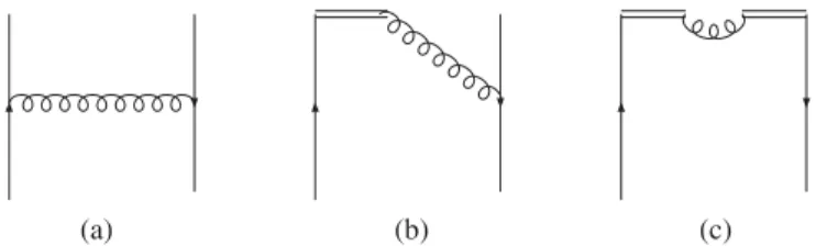
(a) (b) (c)

FIG. 3. Virtual diagram contributions to the Q-TMD quark distributions at one-loop order with quark self-energy (a), quark- gauge-link vertex correction (b) and gauge link self-energy (c).

The complex conjugate is also implied. Diagram (c) requires the renormalization of the gauge link self-interaction. This follows recent examples in the collinear parton quasidistributions cases.

(a) (b) (c)

FIG. 2. Real diagram contributions to the Q-TMD quark distributions at one-loop order with a gluon exchange between quarks (a), between quark and gauge link (b) and between gauge links (c). The complex conjugate of Diagram (b) is implied.

Diagram (c) would contain the pinch pole singularity with infinite

length gauge links in the TMD definition. However, with a finite

length L, this singularity is absent in Q-TMD.

(4)

q

^ð1Þ

ð x _z ; k ⃗

_⊥

Þj

^ðsubÞ_2ðcÞ

¼ q

^ð1Þ

ð x _z ; k ⃗

_⊥

Þj

^ðsubÞ_2ðcÞ

− 1

2 q

^ð1Þ

ð x _z ; k ⃗

_⊥

Þj

^ðsubÞ_2ðcÞ

ð L → 2 L Þ

¼ α s

4π

²

C _F δð1− x _z Þ Z dk _z

k

²

_z

ffiffiffiffiffiffiffiffiffiffiffiffiffiffiffi 1 k

²

_z þ k ⃗

_⊥²

q

× 1

2 ½ð1− e ^ik

^z

^L Þ

²

þð1 − e

^−ik^z

^L Þ

²

: ð 11 Þ In the Fourier transform b ⃗

_⊥

-space, the above result becomes,

q

^ð1Þ

ð x _z ; b ⃗

_⊥

Þj

^ðsubÞ_2ðcÞ

¼ α s

2π C _F δð1 − x _z Þ½2Kðξ b Þ − Kð2ξ b Þ ; ð 12 Þ where the second term comes from the soft factor. Clearly, the linear term of ξ b is canceled out in the subtracted contribution, and the result goes like ln ðξ

²

b Þ at large ξ b , whereas at small ξ b it again behaves like ξ

²

_b .

Similarly, the contribution from Fig. 3(c) is given by (for a finite length gauge link)

q

^ð1Þ

ð x _z ; k ⃗

_⊥

Þj

_3ðcÞ

¼ − ig

²

C _F 2

Z d

⁴

k

⁰

ð2πÞ

⁴

1 ð p − k

⁰

Þ

²

1 ½ n · ð p − k

⁰

Þ

²

× ð1 − e ^in·ðp−k

⁰^ÞL

Þð1 − e

^{−in·ðp−k}⁰^ÞL

Þ

× δð k

⁰

_z − x _z P _z Þδ

^ð2Þ

ð k ⃗

_⊥

Þ : ð 13 Þ After soft factor subtraction, it gives the following expression,

q

^ð1Þ

ð x _z ; k ⃗

_⊥

Þj

^ðsubÞ_3ðcÞ

¼ α s

8π

²

C _F δð1 − x _z Þδ

^ð2Þ

ð k ⃗

_⊥

Þ

Z dk _z d

²

k ⃗

⁰_⊥

k

²

_z

× 1 ffiffiffiffiffiffi

⃗ k

⁰²_⊥

q − ffiffiffiffiffiffiffiffiffiffiffiffiffiffiffiffi 1 k

²

_z þ k ⃗

⁰²_⊥

q

!

×

ð1 − e ^ik

^z

^L Þð1 − e

^−ik^z

^L Þ

− 1

2 ð1 − e ^i2k

^z

^L Þð1 − e

^−i2k^z

^L Þ

; ð 14 Þ where we have rewritten the integral over k ⃗

⁰_⊥

in such a way that the linear divergence is manifestly absent. In addition, all L-dependent contributions that are not sup- pressed in the large L limit cancel out in the full subtracted Q-TMD. The cancellation occurs either among the unsub- tracted Q-TMD diagrams or with similar contributions from the soft factor. This can be easily seen from compu- tations in coordinate space.

As there is no linear divergence associated with the gauge links after soft factor subtraction, we can work in

dimensional regularization, which leads to the following contribution,

q

^ð1Þ

ð x _z ; b ⃗

_⊥

Þj

^ð_3ðcÞ^sub^Þ

¼ α s

4π C _F δð1 − x _z Þ

ln L

²

μ

²

4c

²₀

þ 2

; ð 15 Þ in the Fourier transform b ⃗

_⊥

-space, where the UV diver- gence has been subtracted with MS scheme. In the dimen- sional regulation, the linear divergence is not manifest explicitly in the unsubtracted Q-TMD, and the result is the same as above with a factor of 2. However, if a cutoff scheme is chosen, there will be an explicit linear divergence in the unsubtracted Q-TMD,

q

^ð1Þ

ð x _z ; b ⃗

_⊥

Þj

^ðunsubÞ_3ðcÞ;tot

¼ α s

2π C _F δð1 − x _z Þ

4 − 2π L

a þ 2 ln L

²

a

²

;

ð16Þ whereas the linear divergence is canceled out for the subtracted Q-TMD

q

^ð1Þ

ð x _z ; b ⃗

_⊥

Þj

^ðsubÞ_3ðcÞ;tot

¼ α s

2π C _F δð1 − x _z Þ

2 þ ln L

²

4 a

²

: ð 17 Þ The transverse gauge link contribution can be calculated in complete analogy and we have

q

^ð1Þ

ð x _z ; b ⃗

_⊥

Þj

^ðunsubÞT_3ðcÞ

¼ α s

2π C _F δð1 − x _z Þ

2 − π b ⃗

_⊥

a þ ln b ⃗

²_⊥

a

²

:

ð 18 Þ For the subtracted Q-TMD, the transverse gauge link contribution is canceled out completely,

q

^ð1Þ

ð x _z ; b ⃗

_⊥

Þj

^ðsubÞT_3ðcÞ

¼ 0 : ð 19 Þ Equations (15) to (17) are independent of b ⃗

_⊥

, and therefore will remain the same at large or small ξ b . From the results above, one can easily see that the subtracted result of Fig. 2(c), 3(c) has a residual logarithmic UV divergence,

q

^ð1Þ

ð x _z ; b ⃗

_⊥

Þj

^ðsubÞ_{2ðcÞ;3ðcÞ}

¼ α s

2π C _F δð1 − x _z Þ

ln L

²

μ

²

4 c

²₀

þ 2 þ 2Kðξ b Þ − Kð2ξ b Þ

; ð 20 Þ

in the Fourier transform b ⃗

_⊥

-space with respect to the

transverse momentum ⃗ k

_⊥

, where c

₀

¼ 2 e

^−γ^E

. In the above

equation, we have applied the dimensional regulation for

the UV divergence and renormalize in the MS scheme with

scale μ . If a lattice regulator is adopted, we will obtain the

(5)

same expression with μ =c

₀

¼ 1 =a, where a is the lattice spacing parameter. Because of the above contribution, we will have an additional anomalous dimension contribution from Eq. (20) for the evolution equation of the Q-TMD.

The rest of the real diagrams in Fig. 2 can be calculated by safely taking the large L limit. For example, the contribution of Fig. 2(b) is given by

− ig

²

C _F 2

Z dk

⁰

dk _z

ð2πÞ

⁴

u ¯ ð p Þγ ^z 1 n · ð P − k Þ

1 = k γ ^z

× 1

ðP − kÞ

²

u ð p Þð1 − e ^{in·ðP−kÞL} Þδð k _z − x _z P _z Þ ; ð 21 Þ and leads to the following result

q

^ð1Þ

ðx z ; k ⃗

_⊥

Þj

_Fig:2ðbÞ

¼ α s

4π

²

C _F 1

⃗ k

²_⊥

x _z 1− x _z

ffiffiffiffiffiffiffiffiffiffiffiffiffiffiffiffiffiffiffiffiffiffiffiffiffiffiffiffiffiffiffiffi P _z ð1 − x _z Þ

⃗ k

²_⊥

þ P

²

_z ð1− x _z Þ

²

q þ P _z x _z

ffiffiffiffiffiffiffiffiffiffiffiffiffiffiffiffiffiffiffiffi

⃗ k

²_⊥

þ P

²

_z x

²

_z

q

þ 1

1 − x _z 1 P

²

_z

P _z

ffiffiffiffiffiffiffiffiffiffiffiffiffiffiffiffiffiffiffiffi

⃗ k

²_⊥

þP

²

z x

²

_z

q − P _z

ffiffiffiffiffiffiffiffiffiffiffiffiffiffiffiffiffiffiffiffiffiffiffiffiffiffiffiffiffiffiffiffi

⃗ k

²_⊥

þP

²

z ð1 −x z Þ

²

q

× ð1 −e ^ið1−x

^z^ÞP^z

^L Þ: ð22Þ

However, this additional factor e

^½ið1−x^z^ÞP^z

^L does not con- tribute in the large L limit. It is interesting to note that if we take P _z → ∞ first, the above equation will lead to a divergence of 1 = ð1 − x _z Þ , which is same as the light-cone singularity in the usual TMD definition. Again, the con- tributions from the regions of x _z < 0 and x _z > 1 are power suppressed in the limit j k ⃗

_⊥

j ≪ P _z . The final result from this diagram can be written as,

α s

2π

²

C _F 1

⃗ k

²_⊥

2 x _z

ð1 − x _z Þ

_þ

θðx z Þθð1 − x _z Þ þ δð1 − x _z Þ ln ζ

²

⃗ k

²_⊥

;

ð 23 Þ where ζ

²

¼ x

²

_z ð2 n _z · P Þ

²

= ð− n

²

_z Þ ¼ 4 x

²

_z P

²

_z and we have applied a principal-value prescription to evaluate the second term in Eq. (23).

Because there is no gauge link contribution from Fig. 2(a), its result will be the same as previously calculated in Ref. [41]

q

^ð1Þ

ð x _z ; k ⃗

_⊥

Þj

_Fig:2ðaÞ

¼ α s

4π

²

C _F 1 −ϵ

⃗ k

²_⊥

×

ð1 − x _z Þ ffiffiffiffiffiffiffiffiffiffiffiffiffiffiffiffiffiffiffiffiffiffiffiffiffiffiffiffiffiffiffiffi

⃗ k

²_⊥

þ P

²

_z ð1 − x _z Þ

²

q

þ P _z ð1 − x _z Þ ffiffiffiffiffiffiffiffiffiffiffiffiffiffiffiffiffiffiffiffiffiffiffiffiffiffiffiffiffiffiffiffi

⃗ k

²_⊥

þ P

²

_z ð1− x _z Þ

²

q : ð 24 Þ

In the limit j k ⃗

_⊥

j ≪ P _z , the above result reduces to α s

2π

²

C _F 1 − ϵ

⃗ k

²_⊥

ð1 − x _z Þ : ð 25 Þ

Similar calculations can be performed for the virtual diagrams of Fig. 3(a,b), and the result reads [41]

q

^ð1Þ

ð x _z ; b ⃗

_⊥

Þj

_{3ðaÞ;3ðbÞ}

¼ α s

2π C _F δð1 − x _z Þ

− 1 ϵ

²

− 3

2ϵ þ 1 ϵ ln ζ

²

μ

²

þ ln ζ

²

μ

²

− 1 2

ln ζ

²

μ

²

₂

þ π

²

12 − 2

: ð 26 Þ

Finally, the total contribution of the subtracted Q-TMD quark distribution at one-loop order can be obtained from Eqs. (20), (26) and the Fourier transform of (23), (25),

q

^ðsubÞð1Þ_{Q TMD}

ð x _z ; b ⃗

_⊥

; ζ

²

Þ

¼ α s

2π C _F

− 1

ϵ þ ln c

²₀

⃗ b

²_⊥

μ

²

P q=q ð x _z Þ þ ð1 − x _z Þ þδð1 − x _z Þ

3 2 ln b ⃗

²_⊥

μ

²

c

²₀

þ ln ζ

²

L

²

4 c

²₀

− 1

2 ln ζ

²

b ⃗

²_⊥

c

²₀

₂

þ2Kðξ b Þ − Kð2ξ b Þ

ð 27 Þ

in b ⃗

_⊥

-space, where μ is the renormalization scale in the MS scheme, and P q=q ð x _z Þ ¼ ð

^1þx_1−x²^z_z

Þ

_þ

is the usual splitting kernel for the quark. We would like to emphasize a number of important points here. First, the Q-TMDs only have contributions in the region 0 < x _z < 1 . This is because, as mentioned above, we are taking the physical limit for TMD, i.e., P _z ≫ j k ⃗

_⊥

j . In this limit, the contributions in the region x _z > 1 and x _z < 0 are power suppressed. Second, similar to the previous formalisms for the TMDs, the Q- TMDs contain the double logarithms as indicated in the above equation. From the explicit calculations, we find that these double logarithms depend on the hadron momentum P _z in the parton quasidistributions framework. Therefore, the associated energy evolution, i.e., the Collins-Soper evolution, will depend on P _z not L. Finally, as expected, the Q-TMD at one-loop order contains infrared divergence, which corresponds to the collinear splitting of the quark.

Comparing to the result in Ref. [41], we find an addi- tional term from the soft factor subtraction in the Q-TMD.

This term will lead to a different matching between the

Q-TMD and the standard TMD.

(6)

III. MATCHING TO THE STANDARD TMDS With the above one-loop result for the Q-TMD quark distribution, we can match to the usual TMDs at this order following the procedure of Ref. [7]. However, there is scheme dependence in the usual TMDs to regulate the relevant light-cone singularities [3]. Therefore, a direct matching to the various TMDs will introduce the scheme dependence as well. On the other hand, as demonstrated in Refs. [42 – 44], all TMD schemes lead to the same result after resumming the large logarithms. Therefore, it is more appropriate to carry out the matching between the Q-TMDs and the standard TMDs after the resummation has been performed.

This resummation is carried out by solving the associ- ated evolution equations [3]. For the Q-TMD quark distribution, the relevant Collins-Soper evolution can be derived [41], and the complete resummation result can be expressed in terms of the integrated parton distributions [3],

q

_{Q TMD}

ð x _z ; b ⃗

_⊥

; ζ

²

Þ

¼ e

^−S^q^ðζ;

^b

^⃗^⊥^Þ

e

^−S^q^w^ðζ;μ^L^Þ

Z dx

⁰

x

⁰

f _q ð x

⁰

; μ b Þ

×

δð1 − ξÞ

1 þ α s

2π C _F ð2Kðξ b Þ − Kð2ξ b ÞÞ

þ α s

2π C _F ð1 − ξÞ

; ð 28 Þ

where f _q represents the integrated quark distribution, the Sudakov factors resum the logarithmically enhanced con- tributions with the following form

S ^q ðζ; b ⃗

_⊥

Þ ¼ Z

_ζ2

μ²_b

d μ ¯

²

¯ μ

²

A ln ζ

²

¯ μ

²

þ B

; ð29Þ

S ^q w ðζ ; μ L Þ ¼ Z

_ζ2

μ²L

d μ ¯

²

¯

μ

²

γ w : ð 30 Þ In the above equation, we have chosen the factorization scale μ ¼ ζ, ξ ¼ x _z =x

⁰

, μ b ¼ c

₀

=j b ⃗

_⊥

j, μ L ¼ 2c

₀

=L. A and B are perturbatively calculable coefficients with A ¼ P

i¼1 A

^ðiÞ

ðα s = πÞ ⁱ and B ¼ P

i¼1 B

^ðiÞ

ðα s = πÞ ⁱ , and the one-loop order coefficients can be read off from Eq. (27) as A

^ð1Þ

¼ C _F =2 and B

^ð1Þ

¼ −3C F =4. The additional Sudakov factor S ^q w comes from the soft factor subtraction, and the anomalous dimension at one-loop is given by γ w ¼ − C _F

_2π^α^s

, as can be read off from the coefficient of the ln

^ζ_4c²

^L

₂²

0

term in Eq. (27). Note that we have set the scale for the Wilson line renormalization as μ ¼ ζ as well. In practice, it may depend on how the Wilson lines are renormalized for the lattice computations. The hard coef- ficient in the second row of Eq. (28) contains all remaining one-loop contributions in Eq. (27).

In order to carry out the matching to the usual TMDs, we compute the TMD quark distribution in the standard scheme [3,42 – 44] as well,

q

_TMD

ðx z ; b ⃗

_⊥

; ζ

²

Þ

¼ e

^−S^q^ðζ;⃗b^⊥^Þ

Z dx

⁰

x

⁰

f _q ðx

⁰

; μ b Þ

δð1 − ξÞ½1 þ Oðα

²

s Þ þ α s

2π C _F ð1 − ξÞ

; ð 31 Þ

where ζ

²

represents the hard momentum scale for the TMDs extracted from the experiments, for example, the invariant mass of lepton pair in the Drell-Yan lepton pair production process. We can also define the above standard TMD as that in the Collins 2011 scheme [3]. We would like to emphasize that the Sudakov factor is the same as above.

Notice that in the standard TMD scheme (or Collins 2011 scheme), the hard coefficient vanishes at one-loop order.

Comparing the above two equations, we can read out the matching between the Q-TMD quark distribution and the standard TMD quark distribution as

q

_{Q TMD}

ð x _z ; b ⃗

_⊥

; ζ

²

Þ

¼ e

q

_TMD

ð x _z ; b ⃗

_⊥

; ζ

²

Þ

1 þ α s

2π C _F ð2Kðξ b Þ

− Kð2ξ b ÞÞ

: ð 32 Þ

The above equation indicates that the Q-TMD computed on the lattice can be interpreted as the TMD for phenomeno- logical applications.

IV. DISCUSSIONS AND SUMMARY

Our final result as shown in Eq. (32) has a number of interesting features. First, because the gauge links in the unsubtracted and subtracted TMD contain Wilson line renormalization, we have additional scale evolution expressed in term of e

. If different renormalization is chosen, we will have a different factor. For example, for the cutoff scheme in the lattice calculation, we will have different factor. In practical calculations, we may not need to perform resummation for this term at all.

In the matching coefficient, we have a functional dependence on ξ b . Its contribution depends on the relative size between L and b ⃗

_⊥

. In the nonperturbative region with

⃗ b

_⊥

≫ L, this is a power correction and can be safely ignored. On the other hand, in perturbative region of

⃗ b

_⊥

≪ L, it could lead to a large logarithm. This, however,

will be dominated over by the Sudakov logs of e

^−S^q

. We do

no need worry too much on its contribution. Of course, in

the nonperturbative region of L ≫ b ⃗

_⊥

∼ Λ

QCD

, this term

may become important and needs to be carefully handled.

(7)

If we can vary the gauge link length L in such way, we may be able to avoid this region. Therefore, this additional term does not cause any problem.

To illustrate the above point, we have investigated the behavior of the term 2Kðξ b Þ − Kð2ξ b Þ by plotting it as a function of b ⃗

_⊥

for different choices of L, which implies that an optimal choice of L would be around 2 ∼ 3=P z for a reasonable range of P _z .

To summarize, we have laid out the basic procedure to compute the TMDs from lattice QCD using LaMET or Q-TMDs. We have shown that the finite length of gauge links plays a crucial role to regulate the so-called pinch pole singularities associated with spacelike gauge links in the Q-TMDs. Additional soft factor subtraction improves the theoretical convergence, especially that it cancels out the linear divergence completely. This paves the way to correctly interpret the numerical results in lattice calcu- lations of the TMDs. We have also shown that the energy evolution equation for the Q-TMDs comes from the large momentum of the hadron P _z . At one-loop order, a double logarithm depending on P _z is found in the Q-TMD calculations. The relevant evolution equation and resum- mation can be performed following the TMD formalism. In particular, our results show that the energy evolution does not depend on the gauge link length L.

Our results may provide a justification of the technique set up in previous attempts to calculate the TMDs on the lattice [6]. However, we would like to emphasize that the

Q-TMD depends on longitudinal momentum fraction x.

Integral over x may induce difficulties to interpret the results from lattice calculations.

Further developments shall follow along the direction outlined in this paper. In particular, we would like to apply our method to a realistic calculation of the Q-TMDs on the lattice. This will be considered in future work. Extensions to the Wigner distributions and other nucleon tomography observables are desirable to follow up as well.

ACKNOWLEDGMENTS

We thank Markus Ebert and Iain Stewart for interesting conversations related to the subject of this paper. This material is based upon work partially supported by the Laboratory Directed Research and Development program of Lawrence Berkeley National Laboratory, the U.S.

Department of Energy, Office of Science, Office of Nuclear Physics, under Contract No. DE-AC02- 05CH11231, and within the framework of the TMD Topical Collaboration, and a grant from National Science Foundation of China (X. J.). J. H. Z. is supported by the Sonderforschungsbereiche/Transregio-55 grant

“ Hadron Physics from Lattice QCD ” and by a grant from National Science Foundation of China (No. 11405104).

Y. Z. is also supported by the U.S. Department of Energy, Office of Science, Office of Nuclear Physics, from No. DE- SC0011090.

[1] D. Boer et al., arXiv:1108.1713; A. Accardi et al., Eur.

Phys. J. A 52 , 268 (2016).

[2] J. C. Collins and D. E. Soper, Nucl. Phys. B193 , 381 (1981);

B213 , 545 (1983); B197 , 446 (1982).

[3] J. C. Collins, Foundations of Perturbative QCD (Cambridge University Press, Cambridge, England, 2011).

[4] X. Ji, J. P. Ma, and F. Yuan, Phys. Rev. D 71 , 034005 (2005).

[5] A. Bacchetta, D. Boer, M. Diehl, and P. J. Mulders, J. High Energy Phys. 08 (2008) 023.

[6] B. U. Musch, P. Hagler, J. W. Negele, and A. Schafer, Phys.

Rev. D 83 , 094507 (2011); B. U. Musch, P. Hagler, M.

Engelhardt, J. W. Negele, and A. Schafer, Phys. Rev. D 85 , 094510 (2012).

[7] X. Ji, Phys. Rev. Lett. 110 , 262002 (2013); Sci. China Phys.

Mech. Astron. 57 , 1407 (2014).

[8] H. W. Lin, J. W. Chen, S. D. Cohen, and X. Ji, Phys. Rev. D 91 , 054510 (2015).

[9] C. Alexandrou, K. Cichy, V. Drach, E. Garcia-Ramos, K.

Hadjiyiannakou, K. Jansen, F. Steffens, and C. Wiese, Phys.

Rev. D 92 , 014502 (2015).

[10] J. W. Chen, S. D. Cohen, X. Ji, H. W. Lin, and J. H. Zhang, Nucl. Phys. B911 , 246 (2016).

[11] C. Alexandrou, K. Cichy, M. Constantinou, K. Hadjiyiannakou, K. Jansen, F. Steffens, and C. Wiese, Phys. Rev. D 96 , 014513 (2017).

[12] J. W. Chen, T. Ishikawa, L. Jin, H. W. Lin, Y. B. Yang, J. H.

Zhang, and Y. Zhao, Phys. Rev. D 97 , 014505 (2018).

[13] H. W. Lin, J.-W. Chen, T. Ishikawa, and J.-H. Zhang (LP3 Collaboration), Phys. Rev. D 98 , 054504 (2018).

[14] C. Alexandrou et al., EPJ Web Conf. 175 , 14008 (2018).

[15] J. H. Zhang, J. W. Chen, X. Ji, L. Jin, and H. W. Lin, Phys.

Rev. D 95 , 094514 (2017).

[16] R. Zhang, J.-W. Chen, L. Jin, H.-W. Lin, A. Schäfer, P.

Sun, Y.-B. Yang,J.-H. Zhang, and Yong Zhao (LP3 Collaboration), Nucl. Phys. B939 , 429 (2019).

[17] Y. Q. Ma and J. W. Qiu, Phys. Rev. D 98 , 074021 (2018).

[18] Y. Q. Ma and J. W. Qiu, Phys. Rev. Lett. 120 , 022003 (2018).

[19] X. Xiong, X. Ji, J. H. Zhang, and Y. Zhao, Phys. Rev. D 90 , 014051 (2014).

[20] X. Ji and J. H. Zhang, Phys. Rev. D 92 , 034006 (2015).

[21] X. Ji, A. Schafer, X. Xiong, and J. H. Zhang, Phys. Rev. D 92 , 014039 (2015).

[22] X. Xiong and J. H. Zhang, Phys. Rev. D 92 , 054037 (2015).

[23] H. n. Li, Phys. Rev. D 94 , 074036 (2016).

(8)

Transverse momentum dependent parton quasidistributions Xiangdong Ji,