). This discretization can be reformulated such that the self-interactions of the gauge field are induced by a path integral over

JHEP07(2019)043

Published for SISSA by Springer

Received: May 2, 2019 Accepted: June 27, 2019 Published: July 9, 2019

Induced QCD II: numerical results

Bastian B. Brandt,^a Robert Lohmayer^b and Tilo Wettig^b

aInstitute for Theoretical Physics, Goethe University,

Max-von-Laue-Strasse 1, 60438 Frankfurt am Main, Germany

bInstitute for Theoretical Physics, University of Regensburg, 93040 Regensburg, Germany

E-mail: brandt@th.physik.uni-frankfurt.de,robert.lohmayer@ur.de, tilo.wettig@ur.de

Abstract:

We numerically explore an alternative discretization of continuum SU(N

_c

) Yang-Mills theory on a Euclidean spacetime lattice, originally introduced by Budzcies and Zirnbauer for gauge group U(N

_c

). This discretization can be reformulated such that the self-interactions of the gauge field are induced by a path integral over

N_b

auxiliary bosonic fields, which couple linearly to the gauge field. In the first paper of the series we have shown that the theory reproduces continuum SU(N

_c

) Yang-Mills theory in

d

= 2 dimensions if

N_b

is larger than

N_c−³₄

and conjectured, following the argument of Budzcies and Zirnbauer, that this remains true for

d >

2. In the present paper, we test this conjecture by performing lattice simulations of the simplest nontrivial case, i.e., gauge group SU(2) in three dimensions. We show that observables computed in the induced theory, such as the static

qq

¯ potential and the deconfinement transition temperature, agree with the same observables computed from the ordinary plaquette action up to lattice artifacts. We also find evidence that the bound for

N_b

can be relaxed to

Nc−⁵₄

as conjectured in our earlier paper. Studies of how the new discretization can be used to change the order of integration in the path integral to arrive at dual formulations of QCD are left for future work.

Keywords:

Lattice QCD, Lattice Quantum Field Theory

ArXiv ePrint: 1904.04351

JHEP07(2019)043

Contents

1 Introduction 1

2 Induced pure gauge theory for gauge group SU(Nc) 3

3 Simulation setup and parameter tuning 5

3.1 Simulation setup

5

3.2 Scale setting and parameter matching

5

3.3 Numerical results for the matching

6

4 The static qq¯potential 9

4.1 Effective string theory and analysis strategy

9

4.2 Simulation points and scale setting

10

4.3 Results for the static potential

14

4.4 Extraction of the boundary coefficient

15

4.5 Continuum limit

18

5 The finite-temperature phase transition 21

5.1 Simulation parameters and results for the Polyakov loop

21

5.2 The transition temperature

22

5.3 Order and universality class of the transition

24

6 Conclusions 26

A Simulation details 28

A.1 Update algorithm

28

A.2 Extraction of the static

qq

¯ potential

28

A.3 Error reduction for large loops

30

B Comparison of the matching with perturbation theory 31

1 Introduction

In the strong-coupling limit of lattice gauge theories, gauge fields do not interact directly

with each other, leading to a factorization of the link integrals in the path integral. This

allows both for analytical investigations and for the construction of new simulation algo-

rithms (e.g., [1–5]). Away from the strong coupling limit the self-interactions of the gauge

field need to be taken into account and, with the standard actions, gauge integrals no

longer factorize, spoiling the applicability of these strong-coupling methods. A particular

way to overcome this problem is to reformulate the gauge action in terms of auxiliary de-

grees of freedom so that the gauge fields only couple to these unphysical degrees of freedom

JHEP07(2019)043

rather than among themselves (e.g., [6–9]). In this approach the gauge action is “induced”

in a well-defined limit only after the auxiliary degrees of freedom have been integrated out. Typically this involves taking the limit to an infinite number of fields, rendering the resulting theories impractical for numerical simulations.

In [10], Budczies and Zirnbauer (BZ) developed a method which induces the pure gauge dynamics already for a fixed and small number of auxiliary bosonic fields. The key idea is to give up on the exact reproduction of the Wilson gauge action at finite lattice spacing in favor of an alternative lattice discretization of Yang-Mills theory which allows for a formulation in terms of auxiliary bosons. The vital ingredients for this idea to work are (a) the existence of a continuum limit and (b) its equivalence with continuum Yang-Mills theory. For the “designer action” (or weight factor) introduced in [10], BZ could show these properties for gauge group U(N

_c

) as long as the number of auxiliary bosonic fields,

N_b

is larger or equal to

Nc

. In QCD we are interested in gauge group SU(N

c

) and in [11] (the first paper of this series) we adapted the BZ approach to this case, avoiding a spurious sign problem in the bosonization of the original formulation by a slight reformulation of the original weight factor. In particular, we could show the existence of the continuum limit as long as

N_b

is larger than or equal to

N_c−1 (orN_c−5/4 if we allowN_b

to be non-integer) and the equivalence with SU(N

c

) Yang-Mills theory in the continuum limit. As in the original BZ paper, the latter could be shown in

d

= 2 dimensions if

N_b ≥N_c

(or

N_b ≥N_c−

3/4 if we take

N_b

to be non-integer), but it is a conjecture for

d >

2. A brief review of the main findings from [11] which are of importance in this article is included in section

2.

In the present article we will investigate the conjecture numerically for the simplest nontrivial case, namely SU(2) gauge theory in three dimensions. We simulate both the standard theory with the Wilson plaquette action, which involves a single parameter

β,

and the induced theory with a fixed number of bosonic fields

N_b

, which involves a single parameter

α. We set the scale for both theories by computing the Sommer scale r₀

[12]

from the static quark-antiquark potential. Matching

r0

from both theories gives us a re- lation between

α

and

β. Using this relation we can compare other observables, such as

quantities connected to the static

qq

¯ potential and the finite-temperature phase transition.

We find that the results agree very well already away from the continuum limit and that

the agreement improves as the continuum limit is approached. A preliminary analysis of

data from SU(3) gauge theory in four dimensions shows that the modified BZ method

also works as expected, supporting the universality argument given in [10]. Therefore the

modified BZ method, combined with a suitable strong-coupling approach, can be used to

reformulate lattice gauge theories in a number of different ways. It will be very interest-

ing to explore such reformulations in the future to see whether they may have advantages

over the traditional formulation (and perhaps even solve the sign problem afflicting lattice

QCD at nonzero density). We remark that an exact rewriting of the pure gauge action in

terms of auxiliary fields has recently been achieved with Hubbard-Stratonovich transfor-

mations [13]. This leads to a qualitatively similar reformulation of the theory, even though

the auxiliary fields are rather different. These two types of reformulations can thus be seen

as complementary approaches with different properties concerning possible reformulations

in terms of dual variables.

JHEP07(2019)043

This paper is structured as follows. In section

2

we review the results from the first paper in the series [11]. The matching between the lattice couplings in Wilson’s pure gauge theory and in the induced gauge theory is discussed in section

3. In sections 4

and

5

we compare the results for the static

qq

¯ potential and the deconfinement phase transition, respectively, before we conclude in section

6. The details concerning the simulation al-

gorithms and the extraction of the observables as well as the details of the simulations for comparison between perturbation theory and numerical results presented in [11] are collected in the appendices. First reports of our study have been published in [14,

15].

2 Induced pure gauge theory for gauge group SU(N

_c

)

We start by reviewing the results from [11] which are relevant for this paper. The weight factor of the alternative discretization of Yang-Mills theory, which we denote by “induced pure gauge theory” (IPG), can be written in the form

ω_IPG

[U ] =

Y

p

h

det 1

−α

2

U_p

+

U_p^†i−Nb

,

(2.1)

where we have adopted the notation used in [11]. Here, 0

≤α <

1 is the lattice coupling, the index

p

labels (unoriented) plaquettes,

U_p

is the product of link variables around the plaquette

p, and N_b

is the number of bosonic fields in the bosonized version of the weight factor. The weight factor (2.1) is a reformulation of the original weight factor introduced in [10] so that one obtains a real action after bosonization (cf. section 2.2 in [11]). Note that in this formulation of the theory

N_b

is just a (positive) number and thus can take any non-integer value, while the bosonization is only possible for integer

N_b

. The weight factor is designed in such a way that, for a given value of

N_b

above the bound in eq. (2.2), the continuum limit is obtained when

α →

1.

In [11] we have shown for gauge group SU(N

c

) that IPG approaches a continuum limit for

α→

1 as long as

N_b ≥N_c−

5

4

.

(2.2)

Furthermore, in two dimensions the theory in the continuum limit is equivalent to contin- uum Yang-Mills (YM) theory if

N_b ≥N_c−

3

4

.

(2.3)

For

d >

2 the equivalence is a conjecture based on a universality argument made in [10]. As shown in [11], another way of approaching the continuum limit is to send

N_b → ∞

while keeping

α

constant. In particular, the lattice theory becomes equivalent to pure gauge theory with the Wilson plaquette action [16]

S_W

[U ] =

− β Nc

X

p

Re Tr

U_p

(2.4)

at lattice coupling

β

when sending

α→

0 and

N_b → ∞

while keeping

β ∼N_bα

fixed. We will refer to the lattice theory with action (2.4) as “Wilson pure gauge theory” (WPG).

The phase diagram of IPG theory is shown in figure

1

in the parameter space of

N_b

and

α.

JHEP07(2019)043

0 α 1

N_b ∞

N_c−⁵₄ N_c−⁵₄

PT bound

Nocontinuumlimit

divergent

Figure 1. The conjectured phase diagram of SU(Nc) induced pure gauge theory in the parameter space of the number of bosons Nb and the coupling α. The darker shading in red indicates the approach to the continuum theory, indicated by the red lines. The dashed black line in the lower right corner indicates the bound α= 1/3 below which perturbation theory for Nb → ∞ is valid.

The blue arrows indicate the interesting region for simulations.

In standard discretizations of Yang-Mills theory one can investigate the nature of the continuum limit by using lattice perturbation theory, making use of the fact that the bare lattice coupling

g

goes to zero in the continuum limit. As noted in [11, section 4.1], such an expansion is not possible in IPG theory around

α

= 1 due to the absence of a Gaussian saddle point. An alternative is to expand the theory around the saddle point for fixed

α <

1/3 and

N_b → ∞

and to analytically continue the results to the region where

α→

1.

The associated bound for perturbation theory is shown as the black dashed line in figure

1.

Using this expansion one finds that a suitable definition of the coupling in IPG theory in the region

α→

1 is given by

1

g²_I

=

d₀

(N

_b

)

α

2(1

−α),

(2.5)

where

d0

is a perturbative coefficient. The relation between the couplings

gW

and

gI

in WPG and IPG, respectively, is then given by

1

g²_W

= 1

g_I²

1 +

d1

(N

_b

)g

²_I

+

. . .

(2.6) with another perturbative coefficient

d₁

. The formulas for the coefficients are given in [11, eqs. (4.12) and (4.13)].

We remark that the weight factor (2.1) respects center symmetry, similar to standard

Yang-Mills theory and its discretizations. This is due to the fact that the weight factor is

formulated in terms of the plaquette

Up

, which itself is a center-symmetric object. Center

symmetry is of fundamental relevance for the order of the deconfinement transition, which

we will study in section

5.

JHEP07(2019)043

3 Simulation setup and parameter tuning

We would like to test the conjecture that the continuum limit of IPG reproduces continuum Yang-Mills theory for

d >

2 when the continuum limit exists, i.e., if eq. (2.2) is fulfilled.

To this end, we compare results obtained from IPG and WPG while taking the continuum limit. The first step along the way is to match the bare parameters such that the sim- ulations in IPG and WPG are done at similar lattice spacings

a. In this section we will

discuss the matching for the test case of three-dimensional SU(2) gauge theory. This is the computationally cheapest non-trivial case to test the conjecture. From the theoretical point of view there is nothing special about this particular case, so that the results obtained here can be expected to be relevant also for other values of

d >

2 and

N_c >

2.

3.1 Simulation setup

We consider pure SU(2) gauge theory discretized on a hypercubic lattice, for which the expectation value of an observable

O

is given by

hOi_IPG/WPG

= 1

Z

Z

SU(2)

[dU ]

O[U

]

ω_IPG/WPG

[U ]

.

(3.1) Here,

Z

normalizes

h1i

to unity, and

ω[U

] is the weight factor, which is given in (2.1) for IPG and by

ω_WPG

[U ] = exp

−S_W

[U ] (3.2)

for WPG with the Wilson plaquette action (2.4). In IPG a simulation point is characterized by two parameters,

N_b

and

α, while WPG has only one parameter, β.

For IPG, we are interested in the continuum limit for a fixed small value of

N_b

, i.e., we approach the continuum limit along the blue arrows in figure

1. In particular, we will

perform the tests for

N_b

= 1 and 2. These two cases are convenient to test the bounds in eqs. (2.2) and (2.3) because both cases satisfy the first bound, which guarantees the existence of a continuum limit, while

N_b

= 1 violates the second bound, which guarantees equivalence with YM theory in two dimensions. Following the arguments of section

2, we

do not expect the latter bound to be relevant for

d >

2.

While WPG can be simulated efficiently with the standard combination of heat- bath [17] and overrelaxation updates [18], such algorithms are not available for IPG. We thus use a simple Metropolis algorithm [19] for the simulations, discussed in detail in appendix

A.1.

3.2 Scale setting and parameter matching

We set the scale using the Sommer parameter

r₀

[12]. This definition of the lattice scale

relies on the physical properties of the static

qq

¯ potential, which can be computed using

Polyakov-loop correlation functions, for instance. The details of the extraction of the po-

tential

V

(R) and the Sommer scale

r₀

are discussed in appendix

A.2. Since the change from

WPG to IPG amounts to a change of the gauge action only, the operators relevant for the

JHEP07(2019)043

measurement of the potential, together with their spectral representation (cf. appendix

A.2)

remain unchanged.

We define equivalent lattice spacings by equivalent values of

r₀/a. This means that,

for fixed value of

N_b

, we match the bare parameters

β

and

α

so that

hr0/ai_WPG

(β ) =

hr₀/ai_IPG

(α). When tuned in such a way, observables are expected to differ by lattice artifacts only, as long as we are close enough to the continuum. Note that the resulting functional dependence

β(α) is not unique. A similar matching could have been obtained

using another observable, such as the string tension

σ, for instance. The resulting matching

relations will then differ by lattice artifacts.

The strategy for the matching is the following: we start by fitting the data for

r0

obtained from simulations of WPG to the expression

¹

r₀

(β) = ¯

r₀

+ ¯

r₁β

+ ¯

r₂β².

(3.3) Performing a simulation of IPG at a fixed value of

α

and computing the corresponding value of

r₀

then gives us, via inversion of (3.3), the value of

β

to which this particular

α

should be matched. This procedure results in a number of pairs (α, β) for a given value of

N_b

, which we fit to a suitable parameterization

β(α). The only piece of information we

include in this parameterization is the fact that

β → ∞

should correspond to

α→

1. We write the parameterization in the form of an asymptotic series,

β(α) =

K

X

k=−n

b_k

(1

−α)^k.

(3.4)

Perturbation theory supports the validity of such an asymptotic expansion around

α

= 1 and suggests

n

= 1, see eqs. (2.5) and (2.6). However, away from perturbation theory, it is not clear that the asymptotic expansion still provides a good parameterization of

β(α).

This has to be clarified by comparison with the numerical data, and we shall see below that

n

= 1 indeed provides the best description, in agreement with perturbation theory.

3.3 Numerical results for the matching

In order to compare the continuum approach of the two theories we have performed simu- lations at four

β-values for WPG for which high-precision results for the quark-antiquark

potential are available [20–26], i.e.,

β

= 5.0, 7.5, 10.0, and 12.5. For the simulations of IPG we have estimated the interesting range of couplings via the expectation value of the plaquette. We have then chosen three different couplings in this range for

N_b

= 1 and

N_b

= 2 to measure Polyakov-loop correlation functions and the Sommer parameter. The simulation parameters are given in table

1. All statistical error bars quoted in the following

are Jackknife errors obtained with 100 bins. We have checked explicitly that the error bars and estimates for secondary quantities do not change significantly if we vary the binsize.

1This expression is a simple fit ansatz, i.e., it contains no assumptions on the relation betweenr0 and β. We have tested the robustness of the matching obtained from this particular choice using several other parameterizations and found no significant dependence of the matching coefficients in (3.7) on the choice ofr0(β).

JHEP07(2019)043

Theory Nb coupling size R ts nt ∆sw meas Nsw r0

WPG β 5.00 24³ 2–10 2 5k 2000 3.947(1)(1)

7.50 36³ 2–11 2 5k 2000 6.286(7)(1)

10.00 48³ 4–19 4 5k 1800 8.603(39)(0)

12.50 64³ 4–19 4 5k 1700 10.900(11)(1)

IPG 1 α 0.900 24³ 1–10 2 100k 20 2000 1000 0.14 3.763(1)(2) 0.930 36³ 1–11 4 200k 40 2100 1500 0.10 6.161(2)(1) 0.945 48³ 1–13 6 500k 100 1700 2000 0.08 8.363(3)(1) IPG 2 α 0.650 24³ 1–10 2 100k 20 2000 1000 0.14 3.329(1)(1) 0.750 36³ 1–11 4 200k 40 2000 1500 0.10 5.969(2)(1) 0.800 48³ 1–13 6 500k 100 2000 2000 0.08 8.252(2)(1) Table 1. Simulation parameters and results for the measurements ofr0in pure SU(2) gauge theory with Wilson action (WPG) and induced action (IPG) forNb = 1 and 2. Here,Rgives the range ofqq¯ separations used in the analysis of Polyakov-loop correlation functions,tsis the temporal extent of the L¨uscher-Weisz sublattices,ntis the number of sublattice updates, ∆sw is the number of sweeps separating two sublattice measurements, Nswis the number of sweeps between two measurements, andis the size of the ball for the link proposal. For more details on the algorithms, e.g., the choice of ∆sw and Nsw, see appendixA.

The methodology for the extraction of

r0

introduced in appendix

A.2

relies on the assumption that IPG is a confining gauge theory for

α <

1. This is not guaranteed, but the existence of a minimal coupling after which the theory is confining in the approach to the continuum limit is a necessary criterion for the approach to continuum Yang-Mills theory. The simulations have shown that this is the case for all couplings of table

1

so that we can extract

r₀

and use it for scale setting. The results for

r₀

are also listed in table

1.

The first error is statistical, and the second error is the uncertainty associated with the interpolation. Note that we have kept the volume at

L/r₀&

7 in order to ensure that finite size effects for

r₀

are small. That this is indeed the case can be seen from a comparison of the data presented in table

1

and the results for

r₀

given in [24,

25], whereL/r₀&

10. The different results are in very good agreement within the statistical accuracy.

We start the matching of the two theories by fitting the WPG data to the form given in eq. (3.3). The results are given in table

2. Note that we have added statistical and

systematic uncertainties in quadrature when fitting the data, which likely overestimates the true uncertainties and can thus explain the rather small value of

χ²/dof in the fit.

Using these results as a definition for the behavior of

r₀

with

β, we then try to find a

matching between

β

and

α

which leads to identical values of

r₀

in the two theories. The guideline for the functional form of

β(α) is eq. (3.4). First, it is necessary to determine

the leading-order of the divergence of

β

in the limit

α →

1. To this end the data for

r₀

obtained in IPG are parameterized by eq. (3.3) and the parameters from table

2, with β

replaced by

β

(α) =

b

(1

−α)ⁿ

+

b₀,

(3.5)

JHEP07(2019)043

Fit parameters χ²/dof

WPG eq. (3.3) r¯0 r¯1 r¯2

-0.79(3) 0.957(9) -0.0017(6) 0.01

IPG eq. (3.5) b b0 n

Nb= 1 0.54( 5) -1.0(2) 1.00(1)

Nb= 2 2.51(24) -2.8(4) 0.99(5)

IPG eq. (3.6) b−1 b0 b1

Nb= 1 0.623( 4) -1.78(11) 3.6(7)

Nb= 2 2.453(14) -2.62(12) -0.1(3)

IPG eq. (3.6);b1= 0 b−1 b0

Nb= 1 0.602(1) -1.218( 9) 109

Nb= 2 2.463(4) -2.694(14) 2.2

Table 2. Results for the parameters of the matching fits (see text). If χ²/dof is not given, the parameterizations contain as many parameters as data points.

where

b,b0

, and

n

are free parameters. Note that this is not a fit, since there are as many free parameters as data points. The results for the parameters are listed in table

2. The

important information is that in both cases,

N_b

= 1 and

N_b

= 2, we have

n≈

1 to good accuracy, implying that we can expect the divergence to be a simple pole. This suggests that a suitable parameterization of

β(α) is given by

β(α) = b₋₁

1

−α

+

b₀

+

b₁

(1

−α) +. . .

(3.6) We test this parameterization by comparison to the data, using either all three terms (in which case there is no fit) or setting

b₁

= 0 (in which case we have a fit with one degree of freedom). The resulting parameters are also listed in table

2. We see that the parameters

with

b₁ 6= 0 and b₁

= 0 are in good agreement for

N_b

= 2 while there are some deviations for

N_b

= 1. It appears that this is due to the large correction of the term including

b₁

, which also leads to a large value of

χ²/dof for the fit where b1

= 0 with

N_b

= 1. Even though a

χ²/dof of 2.2 is not satisfactory, the fit for the N_b

= 2 case, in contrast, works reasonably well. Since in both cases the correction term including

b₁

is not negligible (for

N_b

= 2 signaled by

χ²/dof>

2) we take the parameterization with

b₁ 6= 0 for the matching

between

β

and

α,

β(α) =

0.623( 4)

1

−α −

1.78(11) + 3.6(7)(1

−α)

for

N_b

= 1

,

(3.7a)

β(α) =

2.453(14)

1

−α −

2.62(12)

−

0.1(3)(1

−α)

for

N_b

= 2

.

(3.7b)

These relations are valid within the present accuracy for

β(r₀

) through inversion of eq. (3.3)

and up to other systematic effects, such as finite size effects, for instance. In the next section

we will provide an update which improves both on precision and on finite size effects, see

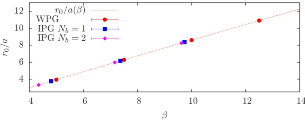
eq. (4.2) below. Figure

2

shows the data for

r₀

vs

β, including also the data from the

induced theory with

β

obtained from (3.7).

JHEP07(2019)043

Figure 2. Results forr0vsβ. Theβ-values associated with the couplingsαfor the induced theory have been obtained using (3.7), which defines the matchingβ(α). The red curve is the interpolating curve (3.3) with the coefficients from table2.

The results from this type of matching can also be compared to the results from perturbation theory obtained in [11]. The comparison between the leading-order coefficient

b₋₁

to the perturbative coefficient has already been done in section 4.3 of [11] and shows an excellent agreement between numerical data and the perturbative prediction, surprisingly even for

N_b

= 1. The details of the comparison and the results for larger values of

N_b>

2 are summarized in appendix

B.

4 The static q q ¯ potential

After matching the bare couplings of WPG and IPG we are now in a position to compare the results for other observables. In this section we will focus on the static

qq

¯ potential, which is not only important to show that the theory is confining but is also related to an effective string theory for the QCD flux tube (for a recent review see [27]). The lat- ter contains non-universal parameters, which can be used to distinguish between different microscopic theories.

4.1 Effective string theory and analysis strategy

A possible way to analyze the static

qq

¯ potential is a comparison to the predictions from the associated effective low-energy theory, namely the effective string theory (EST) for the QCD flux tube, which governs the potential at intermediate and large

qq

¯ separations

R. The interested reader is referred to the reviews [27,28] for further reading about the

foundations of the EST and a thorough list of references.

The main result from the EST that we will use in the analysis is the prediction for the

R

dependence of the static

qq

¯ potential for large

R

[29–33],

V^EST

(R) =

σR

1

−π

(d

−

2)

12σR

² −

¯

b₂π³

(d

−

2) 60

√

σ³R⁴

+

O

(R

^−ξ

)

,

(4.1)

where

σ

is the string tension and

ξ

= 6 or

ξ

= 7, depending on whether the next term in

the large-R expansion originates from another boundary term or a bulk term. The first

JHEP07(2019)043

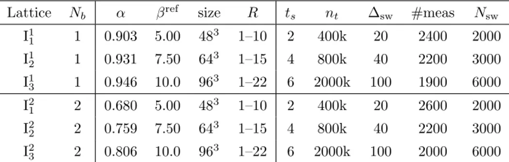
Lattice Nb α β^ref size R ts nt ∆sw #meas Nsw

I¹1 1 0.903 5.00 48³ 1–10 2 400k 20 2400 2000

I¹₂ 1 0.931 7.50 64³ 1–15 4 800k 40 2200 3000

I¹₃ 1 0.946 10.0 96³ 1–22 6 2000k 100 1900 6000

I²₁ 2 0.680 5.00 48³ 1–10 2 400k 20 2600 2000

I²2 2 0.759 7.50 64³ 1–15 4 800k 40 2200 3000

I²₃ 2 0.806 10.0 96³ 1–22 6 2000k 100 2000 6000

Table 3. Simulation parameters for the high-precision measurements of the staticqq¯potential in simulations with the induced action. β^ref is the target value ofβ in WPG theory. The meaning of the other parameters is the same as in table 1. To avoid the propagation of rounding errors, the α-values were computed using all digits ofb−1,b0 andb1 instead of the rounded values in (3.7).

term on the right-hand side is the light-cone spectrum [29], which is expected to appear due to the integrability of the leading-order

S-matrix in the analysis using the thermodynamic

Bethe ansatz [32,

33]. The appearance of the full square-root formula is also in good

agreement with numerical results for the potential (see [27] for a compilation of results).

The parameter ¯

b₂

in eq. (4.1) is the leading-order boundary coefficient [30,

31], which

has been found to be non-universal [25,

26]. In the spectrum, possible corrections to the

standard EST energy levels, such as the rigidity term, first proposed by Polyakov [34], and corrections due to massive modes [32,

33], have been left out.

Our basic strategy is to try to reproduce, and to compare to, the high-precision results from [25], performing the same analysis steps. Since our aim is to perform a like-by-like comparison, rather than validating the string picture, we focus on the basic EST analysis, i.e., sections 3 and 4 in [25].

4.2 Simulation points and scale setting

For the comparison we have performed simulations at bare parameters

α

and volumes that are matched to the parameters in [25] using the matching relations (3.7). The new set of parameters is shown in table

3.

For the purpose of scale setting and to check the matching of eq. (3.7) we have computed the Sommer parameter using the same strategy as before. The results are given in table

4.

We can use these results to update the scaling relation (3.7). For the parameterization with

b₁ 6= 0 we obtain

β(α) =

0.618( 3)

1

−α −

1.63( 9) + 2.5(7)(1

−α)

for

N_b

= 1

,

(4.2a)

β(α) =

2.439(15)

1

−α −

2.48(13)

−

0.5(3)(1

−α)

for

N_b

= 2

.

(4.2b) The above relations are superior to the scaling relations (3.7) in terms of statistical accuracy and finite size effects.

For a first comparison of observables in the approach to the continuum we can look

at the expectation value of the plaquette. Even though trivial in the continuum limit,

JHEP07(2019)043

Lattice r0 Up/Nc Rmin √σ(i)r0 √σ(ii)r0

I¹₁ 3.9264(5)(39) 0.795094(16) 4 1.2292(17) 1.2309(5) I¹₂ 6.2804(6)( 3) 0.865488( 8) 5 1.2398(34) 1.2355(8) I¹3 8.5527(6)( 8) 0.898656( 5) 8 1.2384(26) 1.2357(6) I²1 3.9401(3)(44) 0.790699( 9) 4 1.2340(28) 1.2320(6) I²₂ 6.3121(5)( 3) 0.863568( 5) 5 1.2342(38) 1.2340(8) I²₃ 8.6057(7)( 8) 0.898044( 4) 8 1.2347(27) 1.2346(7)

Table 4. Results for the Sommer parameterr0, the average plaquetteUp, the string tensionσas obtained from methods (i) and (ii) described in the text, for the simulations listed in table3.

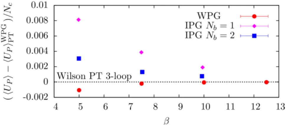
Figure 3. Results forUp/Ncrelative to the perturbative result for the Wilson action of eq. (4.3) vsβ. Theβ-values associated with the couplingsαfor the induced theory have been obtained using eq. (4.2).

its dependence on the lattice spacing, i.e., the bare coupling, is non-trivial and can be computed in lattice perturbation theory. The three-loop result for SU(2) WPG in

d

= 3 is given by [35]

U_p^WPGPT /N_c

= 1

−

0.25g

₀²−

0.01453916(4)g

⁴₀−

0.0053459(2)g

₀⁶.

(4.3) The numerical results for the plaquette are listed in table

4

and shown in figure

3. To

make the small differences visible we do not display the raw data but rather the difference between the plaquette expectation values and the perturbative result.

The plot shows that the WPG results are already very close to the perturbative result,

i.e., lattice artifacts with respect to 3-loop perturbation theory for Wilson’s gauge action

are small. From the plot one might be led to the conclusion that lattice artifacts for IPG

are larger. However, the coefficients of the perturbative result which we subtracted have

been obtained from Wilson’s plaquette action and are expected to be different for IPG

in general, and for different values of

N_b

in particular. Indeed, corrections to eq. (4.3) in

WPG theory start at order

g⁸₀

, while for IPG theory corrections start at lower orders.

JHEP07(2019)043

Another option to set the scale is via the string tension

σ, which governs the linear rise

with

R

of the potential for

R→ ∞. As in [25] we extractσ

with two different methods:

(i) We fit the force to the form

R²F(R) =σR²

+

γ ,

(4.4) motivated by the expansion of the EST potential to next-to-leading-order in 1/R.

(ii) We fit the potential to

V

(R) =

σR r

1

−π(d−

2)

12σR

²

+

V0,

(4.5)

corresponding to the (full) leading-order EST prediction with an additive normaliza- tion constant

V₀

.

This particular combination of ans¨ atze is especially useful since corrections with respect to the full EST prediction, eq. (4.1), appear at different orders in the 1/R expansion. Conse- quently, we can determine the region where higher-order terms in the EST are negligible by comparing the results for

σ

from methods (i) and (ii). The basic strategy is to investigate the dependence of

σ

on the minimal value of

R

included in the fit,

R_min

. In particular, in the region where the results from the two methods agree within errors and show a plateau, higher-order terms are expected to be negligible, and we can use any of the results for

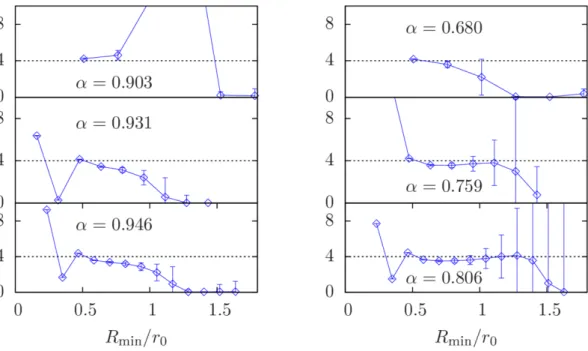
σ.

In figure

4

we show the results for the extraction of the string tension in IPG for

N_b

= 1 (left) and

N_b

= 2 (right). We see that for

N_b

= 1 and

α

= 0.931 and 0.946 the results from method (i) already start to leave the plateau region when the results from method (ii) reach the plateau. Nevertheless, the plateau values agree within uncertainties, as the results from method (i) agree within errors at the point where the results from method (ii) reach the plateau region. As the final results for the string tension, we will use the result from method (ii) obtained with the value of

R_min

where the results of the two methods become consistent. In the cases without a common plateau we use the value of

R_min

where the result from method (ii) starts to agree with the plateau from method (i). The final results are indicated by the red bands in figure

4. The results for σ

are listed in table

4.

The quoted uncertainties for

σ

include the systematic uncertainties for

r₀

, which have been conservatively added in quadrature to the statistical uncertainties.

To compare the results for

σ

with the results for WPG with gauge group SU(2) from [25]

we show the two sets of results in figure

5

for

N_b

= 1 (left) and

N_b

= 2 (right). For

N_b

= 2

we observe good agreement between the results from IPG and WPG, while some slight dif-

ferences are visible for

N_b

= 1. The latter could either be fluctuations, remnants of uncon-

trolled systematic uncertainties connected to the extraction of

σ, or simply due to the dif-

ferent lattice artifacts in the two theories. Eventually, we expect the results to agree in the

JHEP07(2019)043

σa2

α= 0.903

σa2

α= 0.931

σa2

R /r₀ α= 0.946 N_b = 1

σa2

α= 0.680

σa2

α= 0.759

σa2

R /r₀ N_b= 2

α= 0.806 σ

σ

Figure 4. Results for the string tension in IPG forNb= 1 (left) andNb = 2 (right) extracted from method (i), σ(i), and (ii),σ(ii), as explained in the text, vs the minimal value ofR included in the fit,Rminin units ofr0. The red bands are the values of σ(ii) which we use for the further analysis.

Figure 5. Continuum extrapolations of√σ(ii)r0 from IPG forNb = 1 (left) and Nb = 2 (right).

For comparison we also show the results for SU(2) WPG from [25] (red circles) and the associated continuum-extrapolated value (black circle).

JHEP07(2019)043

continuum limit. To test this, we have performed a continuum extrapolation of the form

²

√σr₀

=

√

σr₀cont

+

b_σ,1a r0

2

+

b_σ,2a r0

4

.

(4.6)

As in [25] we perform two fits, either with

b_σ,2 6= 0 or with b_σ,2

= 0. The resulting ex- trapolations are also shown in figure

5

together with the extrapolation for WPG from [25]

(black circle). We see that for

N_b

= 2 the continuum extrapolations are all in very good agreement with the WPG result, even though less precise, which can be expected since only three points are available for the extrapolation. For

N_b

= 1 the extrapolation linear in

a²

overshoots the WPG result. However, the data also indicate the importance of higher-order terms. Including the

a⁴

term leads to an extrapolation which is fully consistent with the WPG result, albeit with large uncertainties. For comparisons we will use the results from the continuum extrapolation with

b_σ,2 6= 0. This extrapolation has larger errors, but the

central value agrees well with the continuum-extrapolated WPG result in both cases.

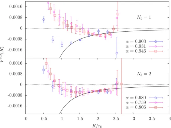
4.3 Results for the static potential

We will now look at the results for the static potential itself. The results for the potential, rescaled according to

V^RS

(R) =

V

(R)

−V₀

√σ −R√ σ

R√ σ π

+ 1

24

,

(4.7)

are shown in figure

6. As in [25] the results for the individual couplings have been rescaled

using the string tension for this value of

α, while the solid line is the rescaled version of

the leading-order EST prediction, the light-cone spectrum, with the continuum limit of the string tension.

Results for the static potential in WPG were already presented in figure 3 of ref. [25].

We do not reproduce that figure here. The comparison with figure

6

shows one of the main problems we are facing, namely the reduced accuracy of the present study, which is mainly due to the less efficient algorithm for IPG compared to the heat-bath algorithm used in the WPG simulations. This leads to a reduction in the range of

R

and reduces the precision in the extraction of

σ. Concerning the results for the potential itself, the agreement with the

WPG results in [25, figure 3] is eminent for

N_b

= 2 and also visible for

N_b

= 1, although the lattice with

α

= 0.903 appears to be outside the scaling region.

³

As in WPG, the corrections to the light-cone potential in IPG are positive and tend to become stronger when approaching the continuum limit.

2Due to the issues with the perturbative investigation of the continuum limit forα→1 (see [11]) it is difficult to obtain information about the powers ofawhich contribute to eq. (4.6) in IPG. However, leading corrections to the Wilson action for Nb→ ∞ at fixedαsimply contain higher powers of (U +U^†−2) in the action. These lead to corrections starting at ordera².

3This can be seen by comparison to the data forβ= 11.0 in SU(3) gauge theory in [25], where a similar behavior occurs.

JHEP07(2019)043

Figure 6. Results for the static potential in its rescaled form, see eq. (4.7), for different lattice spacings vs R for SU(2) IPG withNb = 1 (top) andNb = 2 (bottom). The black continuous line is the light-cone potential obtained with the continuum-extrapolated string tension.

The next step in the analysis is to check whether the leading-order correction to the square-root formula in eq. (4.1) is indeed of order

R⁻⁴

. To this end we fit the data to the form

V

(R) =

σR

1

− π(d−

2)

12σR

²

+

η√

√ σ

σRm

+

V₀,

(4.8)

where

η, m, σ

and

V₀

are fit parameters. If the predictions of the EST are correct, we will obtain

m

= 4. Otherwise we will find

m <

4 if the square-root formula in eq. (4.8) is incorrect, or

m >

4 if the corrections start at higher order. We show the results for

m

vs

R_min

in figure

7. As in SU(2) WPG, cf. [25, figure 4], we typically observe a plateau around

0.5

R/r0

1.0. For

N_b

= 1 the uncertainties are typically larger for larger

R-values, so

that the plateau does not last as long as for

N_b

= 2. The plateau value is typically around

m

= 3.6. This slight discrepancy with expectations has also been found in WPG [25] and indicates a possible mixing with other correction terms. At finite

Nc

the EST will receive corrections from virtual glueball exchange, for instance.

4.4 Extraction of the boundary coefficient

To make the comparison of the subleading properties of the potential more quantitative,

we will now extract the boundary coefficient ¯

b₂

. As in [25], we include higher-order terms

JHEP07(2019)043

Figure 7. Results for the exponentmplotted vs the minimal value ofRincluded in the fit,Rmin, for SU(2) IPG withNb = 1 (left) andNb= 2 (right). The horizontal line indicates the exponent of the leading correction to the EST.

in the fit formula and fit the potential to the form

V

(R) =

V^EST

(R) +

γ₀⁽¹⁾

√σ⁵R⁶

+

γ₀⁽²⁾

σ³R⁷

+

V₀.

(4.9)

Specifically, we perform the following fits [25]:

A

We use

σ

and

V₀

from method (ii) as input and fit with ¯

b₂

,

γ₀⁽¹⁾

and

γ₀⁽²⁾

as free parameters.

B

We use

σ,V₀

and ¯

b₂

as free parameters and set

γ₀⁽¹⁾

= 0 and

γ₀⁽²⁾

= 0.

C

We use

σ,V0

, ¯

b2

and

γ₀⁽¹⁾

as free parameters and set

γ₀⁽²⁾

= 0.

D

We use

σ,V₀

, ¯

b₂

and

γ₀⁽²⁾

as free parameters and set

γ₀⁽¹⁾

= 0.

E

We use

σ,V₀

,

γ₀⁽¹⁾

and

γ₀⁽²⁾

as free parameters and set ¯

b₂

= 0.

The fits are performed for several values of

Rmin

, and we extract the final result from the second smallest

R_min

which provides a

χ²/dof <

1.5. The quality of the agreement with the data is then indicated by the value of

R_min

(smaller values mean better agreement) in context with the number of higher-order terms included in the fit. Fit

C, for instance,

should allow for a smaller value of

R_min

compared to fit

B

since the latter does not contain higher-order correction terms. To check for the systematic uncertainty associated with the fit interval we compare the result to the ones obtained with

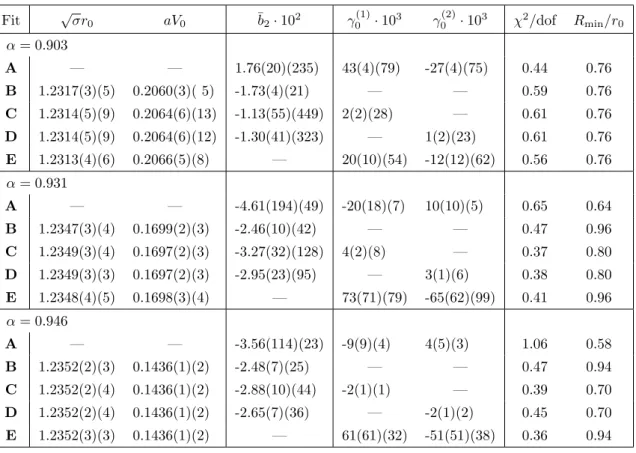
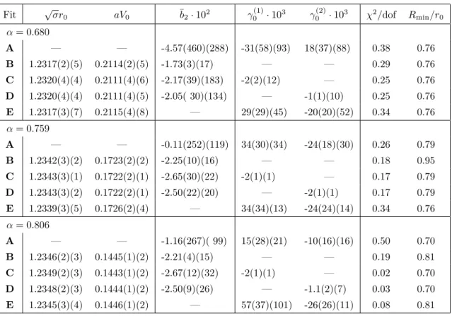
Rmin±a.

We list the results of the different fits for

N_b

= 1 and 2 in tables

5

and

6, respectively.

Comparing the results to those of [25, table 5], in particular for

β

= 5.0, 7.5 and 10.0, we

JHEP07(2019)043

Fit √

σr0 aV0 ¯b2·10² γ₀⁽¹⁾·10³ γ₀⁽²⁾·10³ χ²/dof Rmin/r0

α= 0.903

A — — 1.76(20)(235) 43(4)(79) -27(4)(75) 0.44 0.76

B 1.2317(3)(5) 0.2060(3)( 5) -1.73(4)(21) — — 0.59 0.76

C 1.2314(5)(9) 0.2064(6)(13) -1.13(55)(449) 2(2)(28) — 0.61 0.76 D 1.2314(5)(9) 0.2064(6)(12) -1.30(41)(323) — 1(2)(23) 0.61 0.76 E 1.2313(4)(6) 0.2066(5)(8) — 20(10)(54) -12(12)(62) 0.56 0.76 α= 0.931

A — — -4.61(194)(49) -20(18)(7) 10(10)(5) 0.65 0.64

B 1.2347(3)(4) 0.1699(2)(3) -2.46(10)(42) — — 0.47 0.96

C 1.2349(3)(4) 0.1697(2)(3) -3.27(32)(128) 4(2)(8) — 0.37 0.80 D 1.2349(3)(3) 0.1697(2)(3) -2.95(23)(95) — 3(1)(6) 0.38 0.80 E 1.2348(4)(5) 0.1698(3)(4) — 73(71)(79) -65(62)(99) 0.41 0.96 α= 0.946

A — — -3.56(114)(23) -9(9)(4) 4(5)(3) 1.06 0.58

B 1.2352(2)(3) 0.1436(1)(2) -2.48(7)(25) — — 0.47 0.94

C 1.2352(2)(4) 0.1436(1)(2) -2.88(10)(44) -2(1)(1) — 0.39 0.70 D 1.2352(2)(4) 0.1436(1)(2) -2.65(7)(36) — -2(1)(2) 0.45 0.70 E 1.2352(3)(3) 0.1436(1)(2) — 61(61)(32) -51(51)(38) 0.36 0.94

Table 5. Results of the fits for the extraction of ¯b2 forNb= 1 IPG.

see that both the possible fit ranges and the resulting parameters are very similar. The only exception is fit

A, for which σ

and

V0

have been taken over from section

4.2. Since

the extraction of

σ

and

V₀

was not as accurate as in [25] it is reasonable that this is the main reason for deviations in this particular fit. We can thus follow the discussion of [25]

and conclude that fits

B,C

and

D

can be used in the following analysis. Fit

E

typically requires larger values for

R_min

compared to fits

C

and

D, even though it also includes two

higher-order terms. Thus we conclude that the agreement with the data is worse for fit

E

than for the other fits. In any case, fit

E

only serves as a check that, given the data,

¯

b₂

does not vanish. Compared to [25], where fit

E

clearly showed less agreement with the data, direct conclusions are more difficult here since the IPG data are less precise than those of WPG.

As in [25], we determine the final results for ¯

b2

on the individual lattice spacings

via the weighted average over the results from fits

B

to

D, where the weight is given

by the uncertainties. To estimate the systematic uncertainty due to the choice of

R_min

we repeat the procedure with

Rmin±a

and use the maximal deviation. The results are

tabulated in table

7. Comparing once more to the SU(2) results of [25], which we list for

comparison in table

7

as well, we see that the results are similar in magnitude and have

similar uncertainties. This is particularly true for

N_b

= 2. For

N_b

= 1 the systematic

uncertainties are somewhat larger, but the overall agreement is still good. We show the

results for ¯

b₂

in comparison to the results of [25] in figure

8. One can clearly see the similar

JHEP07(2019)043

Fit √

σr0 aV0 ¯b2·10² γ₀⁽¹⁾·10³ γ₀⁽²⁾·10³ χ²/dof Rmin/r0

α= 0.680

A — — -4.57(460)(288) -31(58)(93) 18(37)(88) 0.38 0.76

B 1.2317(2)(5) 0.2114(2)(5) -1.73(3)(17) — — 0.29 0.76

C 1.2320(4)(4) 0.2111(4)(6) -2.17(39)(183) -2(2)(12) — 0.25 0.76 D 1.2320(4)(4) 0.2111(4)(5) -2.05( 30)(134) — -1(1)(10) 0.25 0.76 E 1.2317(3)(7) 0.2115(4)(8) — 29(29)(45) -20(20)(52) 0.34 0.76 α= 0.759

A — — -0.11(252)(119) 34(30)(34) -24(18)(30) 0.26 0.79

B 1.2342(3)(2) 0.1723(2)(2) -2.25(10)(16) — — 0.18 0.95

C 1.2343(3)(1) 0.1722(2)(1) -2.65(30)(22) -2(1)(1) — 0.17 0.79 D 1.2343(3)(2) 0.1722(2)(1) -2.50(22)(20) — -2(1)(1) 0.17 0.79 E 1.2339(3)(5) 0.1726(2)(4) — 34(34)(13) -24(24)(14) 0.34 0.76 α= 0.806

A — — -1.16(267)( 99) 15(28)(21) -10(16)(16) 0.50 0.70

B 1.2346(2)(3) 0.1445(1)(2) -2.21(4)(15) — — 0.19 0.81

C 1.2349(2)(3) 0.1443(1)(2) -2.67(12)(32) -2(1)(1) — 0.02 0.70 D 1.2348(2)(3) 0.1444(1)(2) -2.50(9)(26) — -1.1(2)(7) 0.03 0.70 E 1.2345(3)(4) 0.1446(1)(2) — 57(37)(101) -26(26)(11) 0.08 0.81

Table 6. Results of the fits for the extraction of ¯b2 forNb= 2 IPG.

WPG IPGNb= 1 IPGNb= 2

β ¯b2 α ¯b2 α ¯b2

5.0 -0.0179( 5)(50)(23) 0.903 -0.0173( 4)(59)(24) 0.680 -0.0174( 4)(43)(19) 7.5 -0.0244(11)(25)(16) 0.931 -0.0260(14)(68)(54) 0.759 -0.0237(16)(28)(14) 10.0 -0.0251( 5)(27)(22) 0.946 -0.0260( 7)(29)(31) 0.806 -0.0233( 6)(35)(19) Table 7. Final results for ¯b2 in WPG [25] and IPG withNb= 1 and 2 for the individual couplings.

The first error is the statistical uncertainty, the second the systematic one due to the unknown higher-order correction terms, estimated by computing the maximal deviations of the results from fitsBtoD, and the third is the systematic one associated with the choice ofRmin.

behavior in the approach to the continuum and the good agreement between the results from the different simulations. In particular, the results are significantly different from the ones for SU(3) gauge theory, showing the discriminating power of the results.

4.5 Continuum limit

Finally, we perform the continuum extrapolation of the boundary coefficient ¯

b₂

. To this end we parameterize it as [25]

¯

b₂

= ¯

b₂cont

+

b¯b2,1

a r₀

2

+

b¯b2,2

a r₀

4

(4.10)

and perform two different types of fits:

JHEP07(2019)043

Figure 8. Results for ¯b2from table7 and for SU(2) WPG from [25] vs the squared lattice spacing in units ofr0. Also shown are the continuum results from eq. (4.11) and the SU(2) result from [25, eq. (6.2)]. The results for SU(2) WPG and for Nb= 2 have been slightly shifted to the left and to the right, respectively, to enable the visibility of the different sets of points.

Nb Fit (1) (2)

1 ¯b2

^cont

-0.0223(37)(40)(44) -0.0276( 9)(31)(47) 2 ¯b2

cont

-0.0214(26)(50)(29) -0.0244( 6)(34)(24) Table 8. Results for ¯b2

cont

from fits (1) and (2) (see text). The first error is the statistical uncertainty, the second the one associated with the unknown higher-order correction terms in the potential and the third the one due to the choice ofRmin.

(1) We fit including all terms in eq. (4.10).

(2) We fit with setting

b¯b2,2

= 0.

Note that fit (1) is a parameterization of the results rather than a fit. In [25] a third fit has been performed, which included only the data for the finest lattice spacings. Such a fit does not make sense here due to the limited number of available couplings. To estimate the propagation of systematic uncertainties we follow the strategy of [25] and perform the fits (1) and (2) for the results from fits

B

to

D

and the fits with a minimal

R-value of Rmin±a

individually. The final results have been extracted using a weighted average of the results from fits

B

to

D, once more with the individual uncertainties as weights. As before,

the individual systematic uncertainties are computed from the maximal deviations to the different fits. The curves for fit (2) with the main value of

Rmin

are shown in figure

9.

The continuum results for ¯

b2

from fits (1) and (2) are given in table

8. We use the

results from fit (1) to estimate the systematic uncertainty associated with the continuum limit. The final results, which we take from fit (2), are thus given by

¯

b₂cont

=

−

0.0276(9)(31)(47)(53) for

N_b

= 1

,

−

0.0244(6)(34)(24)(30) for

N_b

= 2

.

(4.11)

JHEP07(2019)043

Figure 9. Results for the linear continuum extrapolation, fit (2), for the results for ¯b2 obtained from fitsB,CandD(from left to right) for SU(2) IPG with Nb= 1 (top) andNb= 2 (bottom).

Those can be compared to the final continuum estimate for SU(2) WPG from [25], ¯

b2cont

=

−

0.0257 (3)(38)(17)(3)

.

(4.12)

In eqs. (4.11) and (4.12) the first error is purely statistical, the second is the systematic uncertainty due to the unknown higher-order terms in the potential, the third is the one associated with the particular choice for

Rmin

and the fourth is the systematic uncertainty due to the continuum extrapolation. We see that the results from eqs. (4.11) and (4.12) agree well within uncertainties. In addition, the sizes of the individual uncertainties are similar, except for the continuum extrapolation, which, however, is expected since in the IPG analysis ensembles at fewer lattice spacings are available.

We briefly summarize the findings of this section. We have repeated the analysis of

the potential in [25] for IPG and found that in every individual step the results agree

extremely well with WPG, for both

N_b

= 1 and 2. The whole analysis indicates that the

fine structure of the potential in the continuum is indeed identical in IPG and WPG. Hence

we can conclude that, at least for the potential, both theories lead to the same continuum

limit (up to the accuracy of this study). This is also reflected in the significant difference

to the results for SU(3) WPG, which shows the discriminating power of this comparison.

JHEP07(2019)043

Theory Nt volumes couplings # meas Nsw

WPG 4 32², 48², 64², 96² 5.00–7.50 100k IPGNb= 1 4 32², 48², 64², 96² 0.900–0.945 100k–400k 100 IPGNb= 2 4 32², 48², 64², 96² 0.650–0.830 100k–200k 100 WPG 6 48², 72², 96², 144² 8.00–11.50 100k IPGNb= 1 6 48², 72², 96², 144² 0.930–0.950 400k 100 IPGNb= 2 6 48², 72², 96², 144² 0.750–0.850 ∼400k 100

Table 9. Simulation parameters of the finite-temperature runs in 3d SU(2) IPG and WPG theories.

For each volume the simulations have been done on the same values of the coupling. For WPG and Nt= 4 the distance between two β-values was taken to be 0.01 in the region aroundTc(∞), while forNt= 6 we used a distance of 0.05. For IPG theory withNb= 1, the distance between two α-values was taken to be 0.0001 forNt= 4 and 0.00025 forNt= 6, while forNb= 2 we used 0.001 for bothNt= 4 and 6. Away fromTc(∞) we have simulated less frequently. ForNt= 4 the number of measurements varies between the different volumes, and around Tc(∞) we have increased the number of measurements with the volume.

5 The finite-temperature phase transition

So far we have compared properties of IPG and WPG for observables at vanishing tem- perature and found good agreement. We will now show that the agreement prevails for thermodynamic observables. In particular, we will consider the deconfinement transition temperature

Tc

and the ratio of critical exponents

γ/ν. The latter can be regarded as a

measure of the universality class of the transition (we expect a phase transition of 2nd or- der). The fundamental lattice observable that can be used to investigate the deconfinement transition is the absolute value of the Polyakov loop,

h|L|i, the order parameter associated

with the breaking of center symmetry. In particular, we choose a setup which is similar to that in [36] so that we can directly compare to this study.

5.1 Simulation parameters and results for the Polyakov loop

As before, we perform simulations in IPG using

N_b

= 1 and 2. In addition, we also simulate in WPG for a direct comparison of the results. To test the approach to the continuum limit we use two different temporal extents,

N_t

= 4 and 6, for which we vary the temperature

T

= 1/(aN

_t

) by varying the lattice spacing

a

via the lattice couplings

α

and

β. For scale

setting we use the results of section

3. The resulting simulation parameters are listed in

table

9. For N_t

= 6 the volumes have been chosen to match the volumes for

N_t

= 4 in physical units.

The main observables are the absolute value of the Polyakov loop

|L|

= 1

V

X

~ x

Tr

Nt

Y

n0=1

U0

(n

0a, ~x)

(5.1)

and its susceptibility

χ_L

=

V |L|²

− h|L|i²

.

(5.2)

JHEP07(2019)043

Figure 10. Results for the absolute value of the Polyakov loop|L|(top) and its susceptibilityχL

(bottom) atNt= 4 with volumes 32²(left) and 96² (right). The legend is the same for all plots.

For each simulation point we have performed at least 100,000 measurements and increased the number of measurements to about 400,000 in the vicinity of

T_c

, where the autocorre- lations increase due to the approach of a second-order critical point.

The results for

|L|

and

χ_L

vs the temperature in units of the Sommer parameter are shown in figures

10

and

11

for

N_t

= 4 and 6, respectively. We always show the two extremal cases of smallest and largest available volume. The plots show the remarkable agreement between the results of WPG and IPG with

N_b

= 1 and 2. This already indicates the similarity between the corresponding phase transitions. In particular, the volume scaling is equivalent in the different cases so that the universality classes can be expected to be equivalent as well. In the following we will investigate this expectation more quantitatively.

5.2 The transition temperature

We define the critical temperature

Tc

through the peak of the Polyakov-loop susceptibility.

We determine it by fitting a Gaussian to the points in the vicinity of the peak. This

definition assumes a Gaussian form of the susceptibility peak, which will, generically, not

be the case. To account for the associated systematic uncertainty we use the distance

between the two points surrounding the maximum as a conservative error estimate for

T_c

.

We have also checked that the systematic uncertainty associated with the number of points

(symmetrically distributed around the maximum) entering the fit is much smaller than this

estimate for the systematic uncertainty of the results. The results for

T_c

in units of

r₀

are

listed in table

10

for the different values of

N_t

and the different volumes. We have not listed