In the previous lecture, we saw that an MST can be computed in O ( p

Lecture 7

Hardness of MST Construction

In the previous lecture, we saw that an MST can be computed in O ( p

n log

n + D) rounds using messages of size O (log n). Trivially, Ω(D) rounds are required, but what about this O ( p

n log

n) part? The Ω(D) comes from a locality -based argument, just like, e.g., the Ω(log

n) lower bound on list coloring we’ve seen.

But this type of reasoning is not going to work here: All problems can be solved in O (D) rounds by learning the entire topology and inputs!

Hence, if we want to show any such lower bound, we need to reason about the amount of information that can be exchanged in a given amount of time. So we need a problem that is “large” in terms of communication complexity, then somehow make it hard to talk about it efficiently, and still ensure a small graph diameter (since we want a bound that is not based on having a large diameter).

7.1 Reducing 2-Player Equality to MST Con- struction

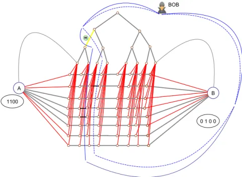
These are quite a few constraints, but actually not too hard to come by. Take a look at the graph in Figure 7.1. There are two nodes A and B, connected by 2k ∈ Θ( √ n) disjoint paths p

, i ∈ { 1, . . . , 2k } of length k, and a balanced binary tree with k + 1 leaves, where the i

leaf is connected to the i

node of each path. Finally, there’s an edge from A to the leftmost leaf of the tree and from B to the rightmost leaf of the tree. This graph has a diameter of O (log k) = O (log n), as this is the depth of the binary tree. Also, it’s clear that all communication between A and B that does not use tree edges will take k rounds, and using the tree edges as “shortcuts” will not yield a very large bandwidth due to the O (log n) message size.

So far, we haven’t picked any edge weights. We’ll use these to encode a difficult problem – in terms of 2-player communication complexity – in a way that keeps the information on the inputs well-separated. We’re going to use the equality problem.

Definition 7.1 (Deterministic 2-Player Equality). The deterministic 2-player equality problem is defined as follows. Alice and Bob are each given N -bit

93

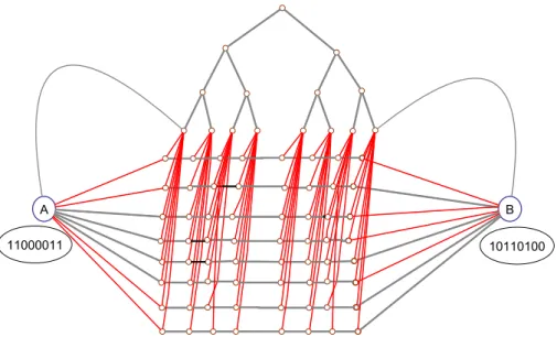
Figure 7.1: Graph used in the lower bound construction. Grey edges have weight 0, red edges weight 1. Only the weight of edges incident to nodes A and B depends on the input strings x and y of Alice and Bob, respectively. The binary tree ensures a diameter of O (log n).

strings x and y, respectively. They exchange bits in order to determine whether x = y or not. In the end, they need to output 1 if and only if x = y. The communication complexity of the protocol is the worst-case number of bits that are exchanged (as function of N ).

Let’s fix the weights. We’ll only need two different values, 0 and 1. Given x, y ∈ { 0, 1 }

, we use the following edge weights:

• All edges between path nodes and the binary tree have weight 1.

• For i ∈ { 1, . . . , k } , the edge from A to the i

path p

has weight x

and the edge from A to p

has weight x

, where x

:= 1 − x

.

• For i ∈ { 1, . . . , k } , the edge from B to p

has weight y

and the edge from B to p

has weight y

.

• All other edges have weight 0.

This encodes the question whether x = y in terms of the weight of an MST.

Lemma 7.2. The weight of an MST of the graph given in Figure 7.1 is k if and only if x = y.

Proof. By construction, the binary tree, A, and B are always connected by edges of weight 0. Likewise, for each i ∈ { 1, . . . , 2k } , the nodes of path p

are connected by edges of weight 0. Hence, we need to determine the minimal

weight of 2k edges that interconnect the paths p

and the component containing

the binary tree, A, and B.

7.1. REDUCING 2-PLAYER EQUALITY TO MST CONSTRUCTION 95 Suppose first that x = y. Then, for each bit x

= y

, either x

= y

= 1 or x

= y

= 1. Thus, either the cost of all edges from p

to the remaining graph is 1, while for p

there are 0-weight edges leaving it, or vice versa. Thus, the cost of a minimum spanning tree is exactly k.

On the other hand, if x 6 = y, there is at least one index i for which x

6 = y

. Thus, both p

and p

have an outgoing edge of weight 0, and the weight of an MST is at most k − 1.

This looks promising in the sense that we have translated the equality prob- lem to something an MST algorithm has to be able to solve. However, we cannot simply argue that if we let A and B play the roles of Alice and Bob in a network, the (to-be-shown) hardness of equality implies that the problem is difficult in the network, as the nodes of the network might do all kinds of fancy things. Similar to when we established that consensus is hard in message pass- ing systems from the same result for shared memory, we need a clean simulation argument.

Theorem 7.3. Suppose there is a deterministic distributed algorithm that solves the MST problem on the graph in Figure 7.1 for arbitrary x and y in T ∈ o( √ n/ log

n) rounds using messages of size O (log n). Then there is a solution to deterministic 2-player equality of communication complexity o(N ).

Proof. We only consider the case where the algorithm requires fewer than k/2 rounds, otherwise it would finish in Ω( √ n) time. Alice and Bob simulate the MST algorithm on the graph in Figure 7.1 for N = k. Alice knows the entire graph but the weights of the edges incident to B and Bob knows everything but the weights of the edges incident to A. In round r ∈ { 1, . . . , T } , Alice simulates the algorithm at the nodes A, the k + 1 − r nodes on each path closest to it, and a subset of the nodes of the binary tree; the same holds for Bob with respect to B.

Because Alice and Bob know only what’s going on for a subset of the nodes, they need to talk about what happens at the boundary of the region under their control. However, since in each round the subpaths they simulate become shorter, the path edges are already accounted for: For the new boundary edges that are in paths, their communication can be computed locally, as the messages that have been sent over them in previous rounds are known – they were in the simulated region!

Hence, we only have to deal with edges incident to nodes of the binary tree.

Consider Alice; Bob behaves symmetrically. In round r, Alice simulates the smallest subtree containing all leaves that connect to path nodes she simulates as well. Observe that this rids Alice and Bob of talking about edges between the tree and the rest of the graph as well. The only issue is now that the “simulation front” does not move as fast within the tree as it does in the remaining graph.

This implies that Alice needs some information only Bob knows: the messages sent to tree nodes by neighbors she did not simulate in the previous round. Since the tree is binary, it has depth d log(k + 1) e ∈ O (log n) and for each node on the

“simulation front,” there is at most one message that needs to be communicated.

Therefore, Alice and Bob can simulate the MST algorithm communicating only O (log

n) bits per round,

provided that T < k/2.

1In Figure 7.2 this only happens for one tree edge per round, because the tree has depth 3;

asymptotically, however, Θ(logn) messages are sent on average.

Figure 7.2: The regions of the graph Alice simulates in rounds 2 (solid purple) and 3 (dotted purple), respectively. Bob needs to tell Alice what message is sent over the yellow edge by the node outside the region of round 2.

Figure 7.3: The regions of the graph Bob simulates in rounds 2 (solid blue) and

3 (dotted blue), respectively. Alice needs to send Bob up to O (log n) bits the

algorithm sends over the yellow edge.

7.2. DETERMINISTIC EQUALITY IS HARD 97 For T < k/2, the subgraphs Alice and Bob have knowledge of cover the graph. Therefore, for a suitable partition of the edge set E = E

∪ ˙ E

, Alice can count and communicate the weight of all MST edges in E

, and Bob can do so for E

. This requires at most 2 log k ∈ O (log n) communicated bits.

By Lemma 7.2, Alice and Bob now can output whether x = y by outputting whether the MST has weight k or not. The total communication cost of the protocol is O (T log

n + log n) ⊆ o(N ).

Remarks:

• In the previous lecture, we required non-zero edge weights. This doesn’t change anything, as picking, e.g., 1 and 2 will change the weight of an MST by exactly n − 1.

• The simulation approach used for Theorem 7.3 is very flexible. Not only can it be used for different weights of the edges incident to A and B, but also for different topologies of a similar flavor. In fact, it is the underlying technique for almost all the non-locality-based lower bounds we know in the distributed setting without faults!

7.2 Deterministic Equality is Hard

We know now that any fast deterministic MST algorithm using small messages implies a protocol solving deterministic equality at small communication cost.

Hence, showing that the communication complexity of this problem is large will yield that MST cannot be solved quickly in all graphs of n nodes, even if D is small.

Theorem 7.4. The communication complexity of deterministic equality is N +1 (respectively N , if we are satisfied with one player learning the result).

Proof. Clearly, N (N + 1) bits suffice: Just let Alice send x to Bob and decide (and tell the result to Alice). Now assume for contradiction that there is a pro- tocol communicating N − 1 bits in which one player decides correctly. As there are 2

> 2

possible values of x, there must be two inputs (x, x) and (x

, x

) (i.e., both with x = y) with x

6 = x so that the sequence of N − 1 exchanged bits (including who sent them)

must be identical. By definition, in both cases the output is 1. Now consider the input (x, x

). By induction on the communicated bits and using indistinguishability, we see that Alice cannot distinguish the ex- ecution from the one for inputs (x, x), while Bob cannot distinguish it from the one for inputs (x

, x

). This is a contradiction, as then one of them decides on output 1, but x 6 = x

implies that the output should be 0. To see that one more bit needs to be communicated if both players need to know the output, observe that for an N -bit protocol, one player would have to decide knowing only N − 1 bits, yielding the same contradiction.

Corollary 7.5. There is no deterministic distributed MST algorithm that uses messages of size O (log n) and terminates in o( √ n/ log

n + D) rounds on all graphs of n nodes and diameter D (unless D is smaller than in the graph from Figure 7.1).

2This follows by induction: Both Alice and Bob must know who sends next, so this must be a function of the transmitted bits.

Proof. Theorem 6.2 shows that running time o(D) is impossible, which shows the claim if D ≥ √ n/ log

n. Theorem 7.3 shows that an o( √ n/ log

n)-round algorithm implied a solution to deterministic equality using o(N ) bits. By The- orem 7.4, this is not possible, covering the case that D ≤ √ n/ log

n.

7.3 Randomized Equality is Easy

One might expect that the same approach extends to randomized MST algo- rithms. Unfortunately, the equality problem defies this intuition: It can be solved extremely efficiently using randomization.

Definition 7.6 (Randomized 2-Player Equality). In the randomized 2-player equality problem, Alice and Bob are each given N -bit strings x and y, respec- tively. Moreover, each of them has access to a (sufficiently long) string of un- biased random bits. They exchange bits in order to determine whether x = y or not. In the end, they need to determine whether x = y correctly with error probability at most ε (for any x and y !).

The communication complexity of the protocol is the worst-case number of bits that are exchanged (as function of N ). We talk of public randomness if Alice and Bob receive the same random bit string, otherwise the protocol uses private randomness (and the strings are independent).

Public randomness is a strong assumption which makes designing an algo- rithm very simple.

Lemma 7.7. For any k ∈ N , randomized equality can be solved with ε = 2

using k + 1 bits of communication assuming public randomness.

Proof. Let a · b := P

i=1

a

b

denote the scalar product over { 0, 1 }

. Consider the probability that for a uniformly random vector v of N bits, it holds that v · x = v · y mod 2. If x = y, this is always true: P [v · x = v · y mod 2 | x = y] = 1.

Otherwise, we have

v · x − v · y mod 2 = v · (x − y) mod 2 = X

i∈{1,...,N}

xi6=yi

v

mod 2,

and as v is a string of independent random bits, P [v · x = v · y mod 2 | x 6 = y]

is the probability that the number of heads for |{ i ∈ { 1, . . . , N } | x

6 = y

}| > 0 unbiased coin flips is even. This is exactly 1/2 for a single coin flip and P [v · x = v · y mod 2 | x 6 = y] = 1/2 can be shown by induction.

In summary, testing whether v · x = v · y mod 2 reveals with probability 1/2 that x 6 = y and will never yield a false negative if x = y. With kN public random bits, Alice and Bob have k independent random vectors. The probability that the test fails k times is 2

. It remains to show that only k + 1 bits need to be exchanged. To this end, Alice sends, for each of the k random vectors v, v · x mod 2 (i.e., 1 bit) to Bob. Bob then compares to y · v for each v and sends the result to Alice (1 bit).

This is great, but what’s up with this excessive use of public random bits? Of

course, we can generate public random bits by communicating private random

bits, but then the communication complexity of the protocol would become

7.3. RANDOMIZED EQUALITY IS EASY 99 worse than the trivial solution! It turns out that there’s a much more clever way of doing this.

Theorem 7.8. Given a protocol for equality that uses public randomness and has error probability ε, we can construct a protocol for randomized equality with error probability 2ε that uses O (log N + log 1/ε) public random bits.

Proof. For simplicity, assume that 6N/ε is integer (otherwise round up). Select 6N/ε random strings uniformly and independently at random and fix this choice.

Now consider an input (x, y) to the equality problem. For most of the fixed random strings, the original protocol will succeed, for some it may fail. Let us check the probability that it fails for more than a 2ε-fraction of these strings.

The number of such “bad” strings is bounded from above by the sum X of 6N/ε independent Bernoulli variables that are 1 with probability ε. Thus, E[X] = 6N.

By Chernoff’s bound,

P[X ≥ 12N] = P[X ≥ 2E[X ]] ≤ e

= e

< 2

.

By the union bound, the probability that there is any pair (x, y) for which there are more than 12N “bad” strings among the 6N/ε selected ones is at most

X

(x,y)

P [X ≥ 12N ] < X

x

X

y

2

= 1.

Thus, with non-zero probability, our choice of 6N/ε random strings is “good”

for all inputs (x, y). In particular, there exists a choice for which this holds! Fix such a choice of 6N/ε (now non-random) strings, i.e., for no (x, y) there are more than 12N strings for which the original algorithm with these strings as “public random bits” outputs the wrong result. Picking one such string uniformly at random and executing the protocol will thus fail with probability at most

12N 6N/ε = 2ε.

We make the list of these strings part of the new algorithm’s code. Alice and Bob now simply pick one entry from the list uniformly at random (using public randomness) and execute the original algorithm with this string as random input. This errs with probability at most 2ε and requires

log

6N ε

∈ O (log N + log 1/ε) public random bits.

Corollary 7.9. Randomized equality can be solved with error probability N

with private randomness and O (log N ) bits of communication.

Proof. We apply Theorem 7.8 to the algorithm obtained from Lemma 7.7 for a choice k ∈ Θ(log N ). We obtain an algorithm using O (log N) bits of public randomness and achieving error probability N

. To make the randomness private, we let Alice choose the Θ(log N ) random bits and communicate them;

this does not affect the asymptotic bit complexity.

Remarks:

• Apart from showing off with Chernoff’s bound, we got to see the probabilis- tic method in action here. We used a probabilistic argument to show that something happens with non-zero probability. Regardless of how small the probability is, it means that there exists some deterministic choice achieving the property that held with non-zero probability.

• Communication complexity people suffer from the same illness as distrib- uted computing folks: They don’t care about local computations.

• Here, this is quite bad. When constructing the algorithm, we cannot be sure that it actually has the desired guarantee on the error probability without explicitly checking for all inputs, which requires exponential com- putations.

• Even if we do this in advance, this causes the additional trouble that we need to assume a bound on N . If Alice and Bob get larger inputs, they are screwed!

• On top of this, Alice and Bob require polynomial memory. The sim- ple algorithm using shared randomness can handle everything using only O (log N ) bits besides the one for the inputs and random bit string.

• In the exercises, you will see a deterministic polynomial time construction.

7.4 Handling Randomization and Approxima- tion

So, equality is not good enough to handle randomization. It also does not cope very well with approximation algorithms, at least not in the construction we’ve seen. We need a communication complexity problem that is hard even for ran- domized algorithms – and ideally, it should yield an all-or-nothing construction for which the MST has non-zero weight only if the answer to the communication complexity problem is “yes.”

Definition 7.10 (2-Player Set Disjointness) . The deterministic and randomized versions of the set disjointness problem are defined as for equality, with the difference that the goal is to decide whether x and y encode disjoint sets, i.e., whether ∃ i ∈ { 1, . . . , N } so that x

= y

= 1.

This problem is hard also for randomized algorithms.

Theorem 7.11 ([KS92, Raz92]). The communication complexity of set dis- jointness is Ω(n), even for randomized algorithms with error probability 1/3.

How can we encode this in our graph? It’s even easier than before:

• Use the same topology, but with only k paths.

• Pick all edge weights as before, except for the edges from Alice and Bob to the endpoints of paths.

• For i ∈ { 1, . . . , k } , the edge from Alice to path p

has weight x

.

7.4. HANDLING RANDOMIZATION AND APPROXIMATION 101

Figure 7.4: How to use the same topology as in Figure 7.1 to encode a set disjointness instance. Now there is a one-to-one correspondence between input bits and paths p

.

• For i ∈ { 1, . . . , k } , the edge from Bob to path p

has weight y

.

Lemma 7.12. The weight of an MST of the modified graph is 0 if and only if x and y encode disjoint sets.

Proof. As before, the question is how expensive it is to connect the paths to the rest of the graph. If x and y encode disjoint sets, then for all i ∈ { 1, . . . , k } we have that x

= 0 or y

= 0, implying that there is an edge leaving the path of weight 0. If the sets are not disjoint, there is a path p

with x

= y

= 1, which therefore cannot be connected to the remaining graph by a 0-weight edge.

Corollary 7.13. There is no distributed MST approximation algorithm that uses messages of size O (log n) and terminates in o( √ n/ log

n + D) rounds on all graphs of n nodes and diameter D (unless D is smaller than in the graph from Figure 7.1).

Proof. Theorem 6.2 shows that running time o(D) is impossible, which shows the claim if D ≥ √ n/ log

n. Analogously to Theorem 7.3, based on Lemma 7.12 we can show that an o( √ n/ log

n)-round algorithm implied a solution to set disjointness using o(N ) bits; this also holds for approximation algorithms, as the weight of the MST is 0 if x and y represent disjoint sets. By Theorem 7.11, this is not possible. This covers the case that D ≤ √

n/ log

n.

• Unfortunately, showing that set disjointness is hard is much more involved than the straightforward argument for deterministic equality.

• In some sense, this bound means that we hit the wall. The hardness comes

from set disjointness, not any fancy aspect of the model.

• On the other hand, one can refine the granularity further by taking into account other parameters. We will see an example for this in a future lecture.

What to take Home

• The machinery demonstrated today produces essentially the same lower bound for plenty of other important graph problems. There will be some examples in the exercises. In some cases, the techniques shows even bounds that are (almost) Ω(n)!

• As a result, communication complexity lower bounds are the tool for show- ing distributed lower bounds arising from congestion. This is very natural, as distributed graph problems are essentially peculiar n-player communi- cation complexity problems, with the addition of a notion of time!

• In many cases, deriving lower bounds of this type is quite easy once one is familiar with the technique. Typically, set disjointness is the source of hardness, Theorem 7.3 works for any graph where the bandwidth available for algorithms between the “input-encoding” parts is small if the running time is small, and all one needs to do is find a suitable graph and encode the instance. Even better: the graph shown works for lots of problems as off-the-shelf topology, only the weights need to be adjusted!

• The probabilistic method, which was only supporting actor today, is also very useful. There are more “constructive” variants, like the celebrated (constructive versions of the) Lov´asz Local Lemma.

• Another bunch of examples for the utility of simulation results. Both derivation of lower bounds and algorithms become easier this way, as ob- stacles are separated and handled in individual steps.

Bibliographic Notes

The first lower bound on MST construction, by Peleg and Rubinovich [PR00], applied only to deterministic exact algorithms. This boils down to the fact that they exploited the hardness of equality, not set disjointness. Elkin [Elk06]

extended the result to randomized approximation algorithms. However, in his construction the lower bound deteriorated depending on the approximation ratio of the algorithm; this was resolved by Das Sarma et al. [SHK

12], who list a large number of related problems for which the technique also yields “the” lower bound of roughly Ω( √ n).

For the basics of communication complexity, see, e.g., [KN97]. The first strong lower bound on the randomized communication complexity of set dis- jointness is due to Babai, Frankl, and Simon [BFS86], showing that Ω( √

N) bits are required. They sampled x and y independently from the N -bit strings with roughly √

N non-zeros. They show that one has to look for more complex distri- butions; essentially, the birthday paradoxon is the monkey wrench in the works.

The Ω(N ) hardness was shown by Kalyanasundaram and Schintger [KS92]; a

simplified proof was given by Razborov [Raz92].

BIBLIOGRAPHY 103 One can dial it up to eleven and show quantum distributed computing com- plexity lower bounds [EKNP14] or derive bounds on multi-party set disjointness in the message passing model [BEO

13], which in turn permits to show hardness by reduction from such problems.

Bibliography

[BEO

13] Mark Braverman, Faith Ellen, Rotem Oshman, Toniann Pitassi, and Vinod Vaikuntanathan. A Tight Bound for Set Disjointness in the Message-Passing Model. In 54th Symposium on Foundations of Com- puter Science (FOCS), pages 668–677, 2013.

[BFS86] Laszlo Babai, Peter Frankl, and Janos Simon. Complexity Classes in Communication Complexity Theory. In 27th Symposium on Foun- dations of Computer Science (FOCS) , pages 337–347, 1986.

[EKNP14] Michael Elkin, Hartmut Klauck, Danupon Nanongkai, and Gopal Pandurangan. Can Quantum Communication Speed Up Distributed Computation? In Proc. 2014 Symposium on Principles of Distrib- uted Computing (PODC), pages 166–175, 2014.

[Elk06] Michael Elkin. An Unconditional Lower Bound on the Time- Approximation Trade-off for the Distributed Minimum Spanning Tree Problem. SIAM Journal on Computing, 36(2):433–456, 2006.

[KN97] E. Kushilevitz and N. Nisan. Communication complexity. Cambridge University Press, 1997.

[KS92] B. Kalyanasundaram and G. Schintger. The Probabilistic Commu- nication Complexity of Set Intersection. SIAM Journal on Discrete Mathematics , 5(4):545–557, 1992.

[PR00] David Peleg and Vitaly Rubinovich. A near-tight lower bound on the time complexity of distributed minimum-weight spanning tree construction. SIAM Journal on Computing, 30(5):1427–1442, 2000.

[Raz92] A. A. Razborov. On the Distributional Complexity of Disjointness.

Theoretical Computer Science, 106(2):385–390, 1992.

[SHK

12] Atish Das Sarma, Stephan Holzer, Liah Kor, Amos Korman,

Danupon Nanongkai, Gopal Pandurangan, David Peleg, and Roger

Wattenhofer. Distributed verification and hardness of distributed ap-

proximation. SIAM Journal on Computing, 41(5):1235–1265, 2012.