Factorization of double parton scattering: The double Drell-Yan process

(1)

Factorization of double parton scattering:

The double Drell-Yan process

DISSERTATION

ZUR ERLANGUNG DES DOKTORGRADS DER NATURWISSENSCHAFTEN (DR. RER. NAT.)

DER FAKULT ¨ AT F ¨ UR PHYSIK DER UNIVERSIT ¨ AT REGENSBURG

vorgelegt von Daniel Ostermeier

aus

Rotthalm¨ unster

im Jahr 2016

(2)

Die Arbeit wurde angeleitet von: Prof. Dr. Andreas Sch¨afer Pr¨ufungsausschuss:

Vorsitzender: Prof. Dr. K. Rincke

1. Gutachter: Prof. Dr. A. Sch¨afer

2. Gutachter: Dr. M. Diehl

weiterer Pr¨ufer: Prof. Dr. F. Evers Termin Promotionskolloquium: 25.04.2016

(3)

Abstract

With the center of mass energy of particle colliders becoming higher and higher multiparton interactions (MPIs) become ever more import and are highly relevant for the LHC. The basis for reliably describing these events based on first principles is built by extending the QCD factorization formalism to multiparton interactions. One of the most important tasks is to show that contributions due to exchange of Glauber gluons cancel in the sum over all diagrams.

In this work we make a contribution to this effort by proving cancellation of Glauber gluon exchange at the one gluon exchange level for the double Drell-Yan process. In doing so, we also review some of the progress made in establishing factorization for MPIs in the last years and indicate how this proof can be extended to all orders in perturbation theory.

(4)

(5)

1. Introduction

With the discovery of the Higgs boson [1, 2], the LHC has provided the last missing piece for eventually verifying the Standard Model. In spite of this great success, the expectations of the physics community were disappointed, because there is still no distinct signal from physics beyond the Standard Model (BSM). Although ATLAS and CMS both might have found first signs of such physics, which they announced in their talks given at CERN on the 15th of December 2015, these signals at around 750 GeV are still very preliminary and could easily be mere statistical fluctuations. BSM physics has to exist, and with run 2 having started at the LHC after its energy upgrade such signals might be discovered soon. At the same time it becomes clearer and clearer that these signals will be rather subtle and that a detailed understanding of the Standard Model background will be indispensable in order to isolate the signals for new physics.

One of the key techniques needed to reliably calculate the QCD background are the so-called QCD factorization theorems, which greatly enhance the predictive power of perturbative QCD (pQCD) [3]. Within the framework of hard scattering factorization, cross sections are calculated as a convolution of parton distribution functions, hard scattering cross sections at the parton level and, in the case of transverse momentum dependent (TMD) factorization, soft factors. There has been lots of effort to prove these factorization theorems to all orders in the strong coupling in pQCD, see e.g. [3, 4, 5]. Some of the approximations used in these studies to arrive at the factorized form of the cross sections are not valid for soft gluon exchange when the gluon momentum is in the so-called Glauber region. Therefore, to validate these proofs it is essential to show that the effects of these Glauber gluon exchanges cancel in the sum over all possible diagrams.

The standard factorization formalism of pQCD is only valid for one hard interaction per hadron-hadron collision. However, with increasing energy the Bjorken x values of partons contributing to reactions with some given ˆs=x₁x₂sdecrease and as the PDFs grow rapidly for smallxmultiple hard interactions become ever more important. At Tevatron they reached already sizeable levels for specific reactions like outgoing (3 jets + γ) or (4 jets), see [6], and for the LHC they are nearly omnipresent, see e.g. [7, 8]. Basically, while multiparton interactions (MPIs) are power suppressed for total cross sections, this is not the case for differential ones, see [9].

Many discovery channels for BSM physics require multiple hard particles in the final state, so they fall in the group of processes especially prone to MPI backgrounds. Obviously theory is called to arms to describe these events reliably, such that pure QCD backgrounds can be subtracted with only small systematic errors. This requires, however, a far reaching extension of present day techniques, and substantial progress has already been made [9, 10, 11].

(10)

As we are interested in differential cross sections, in particular as functions of transverse momenta, one has to develop a multiparton version of TMDs, which by themselves are still faced with open factorization issues. Already for single hard scattering factorization might get broken if hadronic initial and final state interactions occure, like inp+p→2 jets +X[12].

Thus, there is presently absolutely no guarantee that MPIs can be brought under complete theoretical control with all implications this has for the discovery potential of the LHC.

Not to be faced with all of these complications at once, we study in this contribution only the double Drell-Yan process, which is the theoretically cleanest case and does not have any hadronic final state interactions. This process is under complete control in the single scattering case and allows for a generalization to multiparton scattering, serving as a testing ground for developing the theory of multiparton interactions.

As already mentioned, one of the most crucial steps in establishing factorization is to show that contributions due to the exchange of Glauber gluons cancels. In this work, we study the exchange of Glauber gluons in the double Drell-Yan process at the one gluon exchange level.

Our conlusion is that there is no contribution from the Glauber region. We will review some of the progress made in establishing factorization for MPIs [9, 11, 13] on the way.

This work is organized as follows: In chapters 2 and 3 we will give a brief account of the basic concepts of QCD and the hard scattering factorization framework. In chapter 4 we review how the concept of TMDs can be generalized to double parton scattering, how the factorized form of the cross section of double Drell-Yan can be derived at tree level and what the current state of the art of implementing MPIs into the analysis of experimental data is [9]. In the case of perturbatively large transverse momenta, one can calculate splitting contributions to the dTMDs, which we will do in chapter 5. As we will see, these splitting contributions have important consequences for the theory of multiparton interactions, as they lead to conceptual issues regarding the consistent separation of single and double parton scattering. A review of the steps needed to establish factorization of double Drell-Yan beyond leading order is given in chapter 6. In chapter 7 we will then prove the cancellation of Glauber gluon exchange in double Drell-Yan at the one gluon exchange level for two particular toy models and also in general. We then give some example calculations of O(α_S) corrections to dTMDs and the hard scattering part in chapter 8. Finally, we will give the main ideas behind the proof of cancellation of Glauber gluon exchange in the double Drell-Yan process to all orders in chapter 9 [13]. We conclude in chapter 10.

(11)

2. Quantum Chromodynamics

The known microscopic interactions can be classified into electromagnetic, weak, strong and gravitational. Quantum Chromodynamics (QCD) is a relativistic, non Abelian quantum field theory that describes the strong interaction. In QCD there are two types of fundamental fields, namely the fermionic quark fields and the bosonic gluon field. Unlike in the quantum field theory of the electromagnetic interaction, Quantum Electrodynamics (QED), where the fundamental fields correspond to actually observable particles (e.g. electrons and photons), one cannot observe isolated single particles states of quarks or gluons. Instead they always form composite particles, the so-called hadrons, with the quarks being the basic constituents and the gluons transmitting the strong force, binding them together.

An important property of QCD is that while the coupling is strong at typical hadronic scales (∼10⁻¹⁵m), it goes to zero for vanishing distances. This property is called asymptotic freedom and has some important consequences: While one can employ small coupling perturbation theory familiar from QED for small distances, this is not the case for hadronic ones. That means that the bound states of QCD are intrinsically non-perturbative. Thus one cannot make predictions from first principles based on perturbation theory alone, but rather has to employ additional techniques like lattice QCD.

QCD gives rise to an overwhelming amount of phenomena, and we will give a short overview of its formulation and its most important properties in the following. The contents of the next sections can be found in any standard textbook or lecture on QCD and quantum field theories, see e.g. [5, 14, 15, 16].

2.1. The QCD Lagrangian

In spite of the rich phenomenology QCD provides, the Lagrangian describing the whole theory can be written down in only two lines, and in the gauge ∂_µA^a,µ= 0 it reads

LQCD=X

f

ψ¯_f(x) i /D−m_f

ψ_f(x)−1

4G^a_µνG^a,µν

− c

2(∂_µAâ,µ) (∂_νAâ,ν)−ξ¯â(x)∂_µ∂^µξâ(x) +gfâbcξ¯â(x)∂^µ

A^c_µ(x)ξ^b(x)

. (2.1) The first term of the Lagrangian in eq. (2.1) is the fermionic part, where the sum over f indicates the sum over the six known quark flavors of the Dirac spinorsψ_f (up, down, charm, strange, top, bottom). D_µ= (∂_µ+igtâAâ_µ) is the covariant derivative, withtâ (a= 1, . . . ,8) being the generators of the SU(3) color group. They are related to the Gell-Mann matrices λâ by tâ = λâ/2. As is well known, the generators of SU(3) do not commute, which makes

(12)

QCD a non Abelian theory. They obey the relation

[t^a, t^b] =if^abct^c . (2.2)

Note that we have omitted the color indices i, j = 1, . . . ,3 on the quark fields as well as on the covariant derivative and summing over color indices is tacitly assumed. Some important identities for the groups SU(N) that will be relevant for the calculations in this work are given in appendix B. The second term in (2.1) is the gluonic part, where the gluon field strength tensor G^a_µν is given by

Gâ_µν =∂_µAâ_ν−∂_νAâ_µ−gfâbcA^b_µA^c_ν . (2.3) The last term in eq. (2.3) emerges due to the SU(3) group being non Abelian and it leads to three gluon and four gluon vertices, which have no counterpart in QED. It is these additional terms that add some more complications to the quantization of QCD. In particular, the three gluon vertex breaks gauge invariance if not accounted for correctly.

The terms in the second line of (2.1) are the so-called gauge fixing and gauge compensating terms, and they appear due to the following reason: In the path integral formulation of QCD, Green functions (vacuum expectation values of time ordered products of fields) are given by a functional integral

h0|Tf[A, ψ,ψ]¯|0i =N Z

DADψDψ e¯ ^iS[A,ψ,^ψ]^¯f[A, ψ,ψ]¯ . (2.4) On the l.h.s. the fields are the quantum fields of QCD while on the r.h.s. the fields are the corresponding classical fields, where ψ and ¯ψ are Grassmann-valued. The problem with this formulation is that the path integral sums over all possible solutions related by gauge symmetry instead of selecting one of them. In order to solve this overcounting problem and to be able to use the same methods to derive e.g. Green functions from the path integral formulation as in QED, one has to add a gauge fixing term to the Lagrangian and introduce so-called Fadeev-Popov ghost fieldsξ^a, which are unphysical scalar fields that obey the Fermi statistics and are constructed such that they always cancel the unwanted terms corresponding to contributions from unphysical gluon polarizations. These additional terms are given in the second line of (2.1). The Feynman rules of QCD, which are needed for perturbative calculations, can then be derived from the Lagrangian (2.1) and they are given in appendix A.

Note that after the Fadeev-Popov method has been used for gauge fixing, the Lagrangian (2.1) is not gauge invariant, i.e. it is not invariant under the following simultaneous local SU(3) transformations:

ψ_i,f(x)⇒[e⁻îgωâ^(x)tâ]_ijψ_j,f(x), Aâ_µ(x)tâ⇒ −i

g e⁻^igω^b^(x)t^bD_µe^igω^c^(x)t^c. (2.5) This makes the derivation and formulation of generalized Ward identities, which are needed

(13)

2.2. REGULARIZATION AND RENORMALIZATION

ℓ

Figure 2.1.: Quark self energy graph.

grangian (2.1) possesses a different symmetry, namely the so-called BRST symmetry [19, 20].

Regarding the quark and gluon fields, the BRST transformations are just gauge transformations as given in eq. (2.5), and therefore any given gauge invariant operator is also BRST invariant.

2.2. Regularization and renormalization

Just like in QED, ultra-violet (UV) divergences appear when calculating diagrams that contain loops. A simple example is given by the quark self energy diagram depicted in figure 2.1.

Calculating this graph, one sees that it is divergent due to contributions from large loop momentaℓ, i.e. from regions where the two interaction vertices are very close to each other.

These divergences appear due to the fact that QCD does not remain valid up to arbitrary energies, but rather has to be seen as an effective theory which is only valid in an energy regime far away from the Planck scale (∼ 10¹⁹GeV). There, the gravitational interaction and the strong interaction are of comparable strength and thus the assumptions made to construct the quantum field theory formulation of QCD (flat Minkowski space and simple Lorentz transformations) are no longer valid.

Gauge theories like QED and QCD have the crucial property that they are renormalizable, i.e. the occuring UV divergences are at most logarithmic and the theory decouples from the physics at the Planck scale. This can be seen from the observation, that in QCD calculations the logarithmic divergences in the ultraviolet scale Λ_UV always appear together with physical quantities of much lower scale Λ_i≪Λ_UV. The potentially divergent part of the difference in the measurement of this physical quantitiy at two different scales is then given by

log Λ²_i

Λ²_UV −log Λ²_j

Λ²_UV = logΛ²_i

Λ²_j , (2.6)

where the divergence has cancelled between the two terms. Generally speaking, in renormalizable theories like QCD the divergences can be removed by the following procedure:

Regularization of the theory: As a first step, one has to introduce a regulator that renders the theory finite. This can e.g. be done by imposing a cutoff on the loop momenta, but this kind of regularization breaks Lorentz invariance and is rather unsuitable for most calculations.

The most convenient way of regularizing QCD for the purpose of perturbative calculations is the so-called dimensional regularization. Given that the renormalizability of QCD is already proven, one introduces an operation called “d-dimensional integration” with the following properties:

(14)

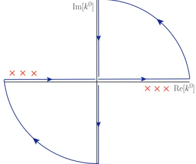
Re[k⁰] Im[k⁰]

Figure 2.2.: Wick rotation of the integration contour in eq. (2.10). When all external momenta are spacelike, the poles in Green functions lie in the 2nd and 4th quadrant and the Wick rotation can be performed.

1. Linearity Z

d^dkE[af(kE) +bg(kE)] =a Z

d^dkEf(kE) +b Z

d^dkEg(kE) (2.7) 2. Translation invariance

Z

d^dkEf(kE +pE) = Z

d^dkEf(kE) for arbitrary finite pE (2.8) 3. Scaling law

Z

d^dk_Ef(λk_E) =λ^−d Z

d^dk_Ef(k_E) forλ∈R (2.9) 4. For all integrands that give at most a logarithmic divergence, the d-dimensional inte-

gration reproduces the result of the Riemann integral in the limit d→4.

Note that all the properties listed above are for Euclidian vectors with k_E² = k²₁ + . . . + k²_d. The usual Lorentz-invariant square of a 4-vector can be related to this via a so-called Wick rotation, which is depicted in figure 2.2. For integrals that are at most logarithmically divergent, the contribution of the arcs vanishes and one can replace

(15)

2.2. REGULARIZATION AND RENORMALIZATION

which impliesk⁰ →ik⁴andk²→ −k_E². In general, such a rotation is only possible for suitable external momenta. One can show that all poles (the red crosses in figure 2.2) of the integrand are in the 2nd and 4th quadrant and thus the Wick rotation can be performed for the case where all external momenta are spacelike. The resulting integral can then conveniently be performed using the master formula

Z

d^dk_E (k_E²)^α

(k_E² +M²)^β =π^d/2(M²)^α−β+d/2Γ(α+d/2)Γ(β−α−d/2)

Γ(d/2)Γ(β) . (2.11)

Note that the corresponding results for external momenta which are not all spacelike are then uniquely defined by analytic continuation. When going from 4 tod= 4−2εdimensions, one introduces an (arbitrary) additional parameterµand replaces the couplinggbygµ^ε. This new parameter is often called renormalization scale. An important property of thed-dimensional integration is that all power divergent intergals, i.e. integrals that diverge stronger than logarithmically, vanish. One can therefore use dimensional regularization only for theories for which such divergences are already known to be absent, as for QCD.

Redefinition of theory parameters: A crucial point is to realize that the parameters (the coupling, the masses of the fields and the field normalizations) appearing in the Lagrangian (2.1) do not correspond to measurable, physical quantities and we will refer to them as “bare”

parameters indicated by a subscript “(0)” in the following. We can use the freedom to redefine the field normalization in the Lagrangian (2.1) as

ψ_(0),f =Z₂^1/2ψ_f, A^µ₍₀₎=Z₃^1/2A^µ ξ₍₀₎= ˜Z^1/2ξ , (2.12) where Z₂, Z₃ and ˜Z are the wave function renormalization factors for the quark fields, the gluon fields and the ghost fields, respectively. One can then absorb the dependence on the ultra-violet cutoff into the bare parameters and the wave function renormalization such that the bare parameters are functions of the physical parameters and the cutoff. In order to obtain finite Green functions (only the Green functions of renormalized fields have to be finite), appropriate counterterms have to be added to the Lagrangian. These counterterms are designed such that they exactly cancel the appearing UV divergences in one-particle- irreducible graphs like in figure 2.1. As the requirement that the divergent parts cancel does only determine the divergent but not the finite part of the counterterms, there is still some freedom of choice. Rules for determining the finite part are called renormalization prescriptions. For calculations in perturbative QCD in many cases the modified minimal subtraction (MS) scheme is used, where one essentially subtracts the term proportional to [5, 21]

1 εS_ε= 1

ε

(4π)^ε Γ(1−ε) = 1

ε + log(4π)−γ_E+O(ε). (2.13) The physical limit: Now that the UV divergences have canceled, one can take the limit ε→ 0. Note that in doing so, the bare parameters become singular such that the physical parameters remain finite, though with a dependence on the renormalization scaleµ.

(16)

2.3. Running coupling, asymptotic freedom and confinement

An important property of quantum field theories like QED and QCD is that the physical parameters, in particular the coupling “constants” e and g, are not constant but rather depend on the scale at which they are measured. In QCD, this leads to the two famous effects called asymptotic freedom and confinement.

This so-called running of the coupling can be obtained in next-to-leading order by calculating all one loop corrections to the quark-gluon vertex. When the quarks are taken to be massless, the result for the sum over all diagrams is

g=g₍₀₎

"

1 + g²₍₀₎ 16π²

1

ε+ log µ²

−k² 11

6 N −1 3N_f

#

, (2.14)

where k is the momentum of the gluon, N is the number of colors andN_f is the number of quark flavors with mass squared much smaller than −k². Using that the difference between the bare coupling and the renormalized coupling is of order g³₍₀₎, one obtains the following differential equation for g:

dg(k²)

d log(−k²) =− g² 16π²

11 6 N −1

3N_f

+O(g⁵). (2.15)

This differential equation is solved by

g(k²) = g(˜µ²) 1 +^g(˜_16π^µ²2⁾ 11

3N− ²₃N_f log

−k²

˜ µ²

, (2.16)

where ˜µ² and g(˜µ²) are integration constants. Using the condition g(˜µ²)

16π² 11

3 N−2 3N_f

log Λ²_QCD µ˜²

!

=−1 (2.17)

these two integration constants can be absorbed into one and the final result for the running coupling αS =g²/4π then reads

α_S(k²) = 4π

11

3 N−²₃N_f log

−k² Λ²_QCD

. (2.18)

So Λ_QCD obviously is the physical scale where the strong coupling becomes singular, and its value is around 200−250 MeV. The final expression for the running coupling (2.18) has some remarkable implications. On one hand, this result has been calculated using massless quarks and yet one arrives at an expression containing a physical dimensionful parameter Λ_QCD. This implies, that the conformal symmetry, i.e. the symmetry under scale transformations, is broken even in massless QCD. On the other hand, one can see already from eq. (2.15) that the coupling decreases with increasing absolute value of transferred momentum squared. This implicates that, at high enough scales, the coupling becomes small enough for perturbation

(17)

2.3. RUNNING COUPLING, ASYMPTOTIC FREEDOM AND CONFINEMENT

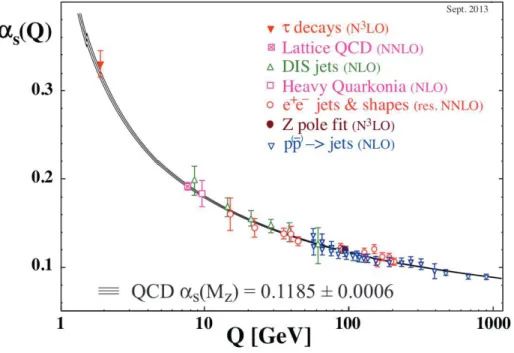
Figure 2.3.: Summary of measurements of αS as a function of the energy scale Q. The respective degree of QCD perturbation theory used in the extraction ofαS is indicated in brackets (NLO: next-to-leading order; NNLO: next-to-next-to leading order; res. NNLO: NNLO matched with resummed next-to-leading logs; N³LO: next-to-NNLO). This plot is taken from [22, chapter 9].

leads to the effect often referred to as confinement: One cannot observe free quarks or gluons, because when trying to separate them the interaction energy becomes large enough to create new quark-antiquark pairs, leading to the formation of new hadrons.

Eq. (2.18) is only the expression for the running coupling at one loop. One can, of course, also calculate higher order corrections. Defining the so-calledβ-function, the differential equation for the running coupling then reads

β = d

d logµ²α_S(µ²) =−β₀

4πα²_S− β₁

8π²α³_S− β₂

128π³α⁴_S+. . . (2.19) with coefficients

β0= 11−2

3N_f, β1 = 51− 19

3 N_f, β2= 2857−5039

9 N_f +325

27 N_f², (2.20) which are given for the number of colorsN = 3 and β₂ is given in the MS-scheme. One can now compare the predictions of these calculations with various experimental measurements of α_S, and this leads to the famous plot of the running coupling of QCD given in figure 2.3. The growth ofα_S at small Qimplies that perturbative calculations are only viable above a scale ofµ² ∼4GeV². Below this scale, different techniques like lattice QCD have to be applied.

(18)

2

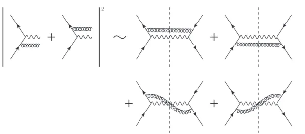
Figure 2.4.: Diagrammatic representation of the Cutkosky cutting rules (2.23). The dashed line denotes the final state cut.

2.4. Cut diagrams

For practical calculations it is often useful to not calculate amplitudes but to organize them in terms of cut diagrams. Due to the unitarity of theS-matrix S= 1 +iT it holds

T^†T =−i(T−T^†). (2.21)

The Cutkosky cutting rules [23] state, that this is equal to the sum over all internal cuts, i.e.

T^†T =−i(T−T^†) =−X

C

TC. (2.22)

A squared amplitude can then be calculated as X

X

hi|T^†|XihX|T|ii=hi|T^†T|ii=hi| −X

C

TC|ii. (2.23) Taking the single gluon emission correction to the Drell-Yan production of a muon pair at the parton level as an example, the diagrammatic identity corresponding to the Cutkosky rule (2.23) is given in figure 2.4. In order to obtain the complete result for the O(α_S) correction to the cross section, one has to add further diagrams corresponding to no gluon emission, i.e.

self energy diagrams and vertex corrections. In calculations the usual Feynman rules given in appendix A are to be applied to the left of the final state cut. The corresponding Feynman rules for lines to the right of the final state cut are obtained by complex conjugation.

(19)

3. Hard scattering factorization

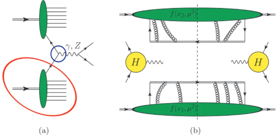
As we have explained in the previous chapter, the strong coupling is only small at sufficiently high energies, or, equivalently, at sufficiently small distances. However, when calculating cross sections of, e.g., proton-proton scattering, there are contributions from both small distances and large distances of hadronic size. This means that these cross sections cannot be calculated completely using only perturbation theory. A way out of this dilemma is given by the so- called factorization theorems, which we will explain for the example of a simple QCD process, namely the Drell-Yan production of a muon pair pp → µ⁺µ⁻X depicted in figure 3.1(a).

Given that we will treat the individual steps of the derivation of the factorization theorem for the double Drell-Yan process in quite some detail in the following chapters, we will only outline the main ideas behind the factorization theorems here.

3.1. Collinear factorization

We first look at the case where only the longitudinal momenta q^± = ^√¹

2(q⁰ ±q³) of the produced muon pair are measured. The momenta of the beam remnants as well as the transverse momentumq= (q¹, q²) are not measured, i.e. they are integrated over. When the µ⁺µ⁻ pair has high invariant mass, the production of the photon can be described by the interaction of one constituent (parton) out of each proton. At leading order in the strong coupling, this is just the quark-antiquark annihilation depicted in figure 3.1(a).

The basic idea behind the factorization approach now is to seperate the whole process into two parts: A nonperturbative part that describes the long-distance dynamics of the process (red circle) and a parton level hard scattering part that depends on the short distance dynamics of the process and that can be calculated in perturbation theory (blue circle). It has been proven that, if the process is sufficiently inclusive, the cross section can approximately be written as [3]

dσ

dQ²dy =X

i,j

Z 1 0

dx₁ Z 1

0

dx₂f_i(x₁, µ²)f_j(x₂, µ²)dˆσ(x₁, x₂, i, j, µ²)

dQ²dy , (3.1)

where y = ¹₂log^q_q⁺₋ is the rapidity of the produced muon pair and Q is its invariant mass.

Corrections to the cross section (3.1) are suppressed by powers of Λ/Q, where Λ is a typical hadronic mass scale.

The parton distribution functions (PDFs)f_i(x_n, µ²) represent the long distance dynamics of the process and are inherently non-perturbative objects. They only depend on the fraction of large longitudinal momentumx_n carried by the respective parton and the factorization scale µ, while the dependence on the transverse momenta and the other longitudinal momentum is integrated out. The PDFs represent the probability of finding a parton of species i with a momentum fractionxn inside of the target and they are independent of the process under consideration, i.e. they are universal. The partonic cross section dˆσ(x₁, x₂, i, j, µ²)/(dQ²dy),

(20)

γ, Z

(a)

H H

f(x₁, µ²) f(x₂, µ²)

(b)

Figure 3.1.: Drell-Yan production of an electroweak gauge boson: (a) full diagram; (b) factorized form of the cross section in the framework of collinear factorization.

by contrast, depends on the process under consideration and can be calculated in perturbation theory. The factorized form of the cross section (3.1) is illustrated in figure 3.1(b).

At tree level, the parton distribution of an unpolarized quark inside the right-moving proton is then defined by the matrix element [5]

f_i(x₁) =

Z db⁻

2π e⁻^ix¹^p⁺^b⁻hp|ψ¯_i(0, b⁻,0)γ⁺

2 ψ_i(0)|pi, (3.2) where p is the momentum of the right-moving proton. We note that this definition is not gauge invariant and is to be amended with suitable so-called Wilson lines (the double lines in figure 3.1(b)) once QCD corrections are taken into account.

Once factorization theorems like (3.1) are proven, this adds a tremendous amount of predictive power to perturbative QCD. One can determine the parton distribution functions from a suitable process like Deep Inelastic Scattering (DIS) and can then use these results for any other process that has been proven to be factorizing. One only has to calculate the hard part, i.e. the parton level cross section, of the process under consideration and obtains a prediction for the cross section.

3.2. TMD factorization

There are many cases where the collinear factorization formalism outlined in the previous section cannot be applied, in particular when details of the final state such as transverse momenta are measured. For these cases, the formalism has to be extended to parton distribution functions where the dependence on the intrinsic transverse momenta of the partons is not integrated out, so called tranverse momentum dependent parton distribution functions (TMDs).

(21)

3.2. TMD FACTORIZATION

An intuitive definition of a TMD for an unpolarized quark of flavoriinside of a right-moving proton is obtained by keeping the transverse momentum dependence of the usual PDFs defined in eq. (3.2),

fi(x,k, µ²)=^?

Z db⁻

(2π)e^−ixp⁺^b⁻

Z d²b

(2π)²e^ik·bhp|ψ¯i(0, b⁻,b)γ⁺

2 ψi(0)|pi, (3.3) where the “?” indicates that this will not be the final definition [5]. The corresponding factorization theorem at tree level reads

dσ

dx₁dx₂d²q = 1 2q²

X

i,j

Z

d²k₁d²k₂δ⁽²⁾(q−k₁−k₂)×

×f_i(x₁,k₁, µ²)f_j(x₂,k₂, µ²)H_ij(x₁x₂s, µ²), (3.4) where H describes the hard scattering at parton level. Indeed, the definition (3.3) and the factorization formula (3.4) are sufficient at tree level, but they are not sufficient for a treatment of the process in full QCD. On one hand, the operator in (3.3) contains two quark fields at different positions. As is well known, such operators are not gauge invariant unless the two quark fields are joined by a gauge link, a so-called Wilson line. On the other hand, one has to allow for additional gluon exchange, which will lead to major changes in the definition (3.3) and the factorization formula (3.4). We will not discuss all these issues here, but will treat them in the context of double Drell-Yan in chapter 6.

(22)

(23)

4. Double Drell-Yan: Lowest order analysis

As already mentioned in chapter 1, with center of mass collision energies becoming higher and higher, an ever smaller value of Bjorken x of the partons inside a proton is enough to contribute to reactions at a specific scaleQ² =x₁x₂s. As the PDFs and TMDs grow rapidly for small x, the probability for two or more hard interactions rises dramatically. A theoretically sound understanding of these multiple interactions is indispensable in order to be able to calculate and subtract the QCD background when searching for signals from BSM physics.

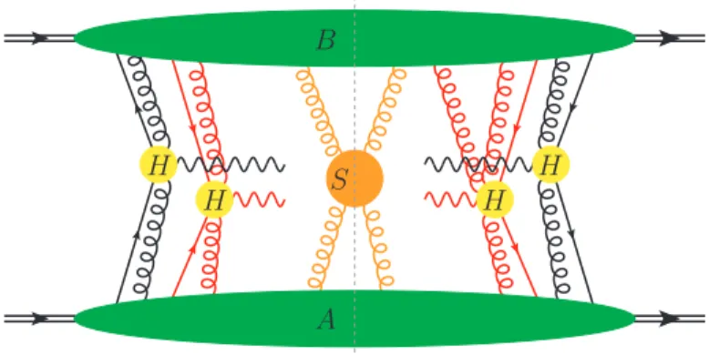
This requires substantial extension of the techniques used for the calculation of cross sections within the single parton scattering framework, and especially of the collinear and TMD factorization procedure. Given that there are substantial difficulties with proving factorization theorems and even explicit violations of TMD factorization in processes with hadrons in both the initial and final state, see e.g. [12], we will restrict our analysis to the most simple case of double parton scattering, namely the double Drell-Yan process depicted in figure 4.1. This process serves as an ideal starting point for the development of the theory of multiple interactions, as its single parton scattering counterpart is completely understood.

In this chapter we will derive the factorized form of the cross section of the double Drell- Yan process in lowest order of the strong coupling. We will restrict ourselves to cross sections differential in transverse momenta. Similar derivations for cross sections integrated over transverse momenta have been given in the past, cf. [24, 25].

In section 4.1 we give the definitions of the double parton distributions, paying special atten- tion to the color and spin structure. In section 4.3 we derive the factorized form of the cross section at lowest order and compare the cross sections of single and double parton scattering with power counting methods. We conclude this chapter with a brief account of the current state of the art of implementing double parton scattering into the analysis of experimental data in section 4.4. Throughout this chapter, we will closely follow the nomenclature, derivations and reasoning of [9].

4.1. Definition of two-parton distributions

We start with defining the two-parton distributions that will appear in the cross section of the double Drell-Yan process depicted in figure 4.1. Note that the following definitions are only valid at lowest order in the strong coupling. At higher orders, these definitions have to be supplemented with appropriate Wilson lines that ensure gauge invariance, and the resulting cross sections contain additional so-called soft factors. We will deal with these complications in chapter 6.

4.1.1. Scalar distributions

We will first give the definition of a two-parton distribution for (hypothetical) scalar partons described by a Hermitian fieldφ. In this case one doesn’t have to deal with the complications

(24)

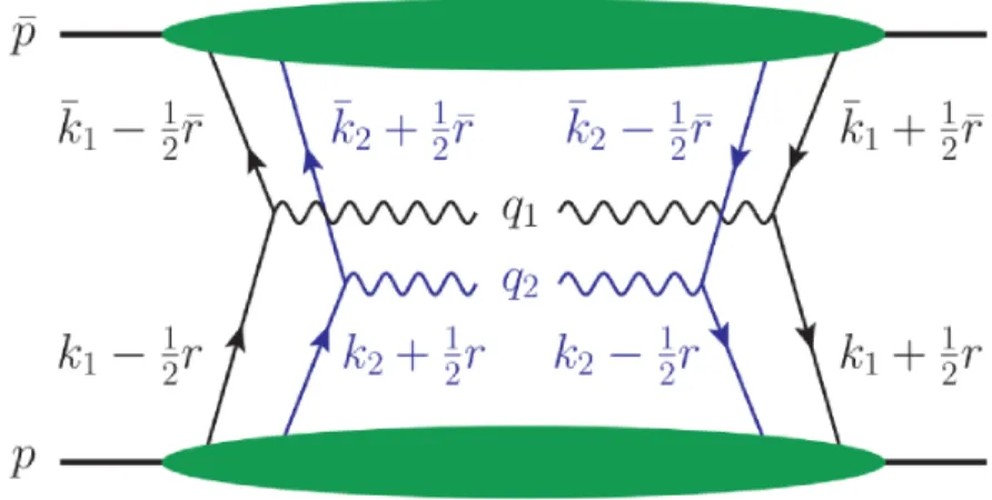
Figure 4.1.: Momentum assignement for the double Drell-Yan process at lowest order in the strong coupling.

that arise due to the parton spin of quarks and gluons in QCD. The starting point for the derivation of the scalar distributions is the two-parton correlation function, which describes the emission of two partons in the scattering amplitude and the absorption of two partons in its conjugate. The definition reads

Φ(l_i, l_i^′) =

Z d⁴ξ₁ (2π)⁴

d⁴ξ^′₁

(2π)⁴ e^iξ¹^l¹^−iξ^′¹^l^′¹

Z d⁴ξ₂

(2π)⁴ e^iξ²^l² p

T¯

φ(0)φ(ξ₁^′)

T

φ(ξ₁)φ(ξ₂)

p , (4.1) where T and ¯T denote time-ordering and anti-time-ordering of the fields, respectively. Due to momentum conservation, the parton momenta have to fulfill the condition l₁+l₂=l₁^′ +l₂^′. Switching to symmetric variables, the structure of the cross section becomes more clear. We first use translational invariance to shift all field positions by−¹₂ξ₂ and then replace

l_i =k_i−¹₂r , l^′_i=k_i+¹₂r (4.2) for the momentum variables and

y+¹₂z₁ =ξ₁−¹₂ξ₂, y−¹₂z₁ =ξ₁^′ −¹₂ξ₂, z₂ =ξ₂ (4.3) for position variables. The resulting expression for the two parton correlation function is

Φ(k_i, r) = 2

Y

i=1

Z d⁴z_i (2π)⁴e^izⁱ^kⁱ

Z d⁴y (2π)⁴ e^−iyr

(25)

4.1. DEFINITION OF TWO-PARTON DISTRIBUTIONS

We now define the transverse momentum dependent two-parton distribution function (dTMD) as

F(x_i,k_i,r) = 2

Y

i=1

k_i⁺ Z

dk_i⁻

(2π)³2p⁺ Z

dr⁻Φ(k_i, r)

k⁺_i=x_ip⁺, r⁺=0

, (4.5)

which can be rewritten as F(x_i,k_i,r) =

" ₂ Y

i=1

Z dz_i⁻

2π e^ixⁱ^zⁱ⁻^p⁺

Z d²z_i

(2π)²e^−izⁱ^·kⁱ

# 2p⁺

Z

dy⁻d²ye^iy·r

× hp|O(0, z₂)O(y, z₁)|pi (4.6)

with the abbreviation

O(y, zi) =φ y− ¹₂zi i 2

−→

∂ −←−

∂+

φ y+¹₂zi

z_i⁺=y⁺=0 . (4.7) Note that in (4.6) we have replaced the time-ordered and anti-time-ordered products by usual products. This can be done, because the position arguments of the fields have a plus- component that is zero. The fields therefore have spacelike seperation and commute because of causality.

4.1.2. Quarks

The starting point for the definition of the two-quark parton distribution is the correlation function for two quarks entering the hard scattering, which is defined by

Φ_α₁_β₁_α₂_β₂(k_i, r) =

" ₂ Y

i=1

#Z d⁴y (2π)⁴e^−iyr

× hp|T¯

¯

q_β₁(y−¹₂z1)¯q_β₂(−¹₂z2) T

qα2(¹₂z2)qα1(y+¹₂z1)

|pi, (4.8) whereα_i and β_j are Dirac indices andT denotes time-ordering whereas ¯T denotes anti-time- ordering, as is appropriate for the quark fields in the amplitude and its conjugate, respectively.

Moreover, we only consider unpolarized hadrons and therefore averaging over the proton spin is tacitly assumed in (4.8). Integrating the correlation function over the parton minus- momenta, we can omit the anti-time and time-ordering due to the spacelike separation of the fields. Thus we can bring them into the following order by an even permutation yielding no change of sign:

¯

q_β₁(y−¹₂z₁)q_α₁(y+¹₂z₁)¯q_β₂(−¹₂z₂)q_α₂(¹₂z₂). (4.9) The Dirac indices of the correlation function are contracted with the indices of the hard scattering matrices H_1,β₁_α₁ and H_2,β₂_α₂. The next step is to expand the hard scattering matrices in a Clifford basis:

H_i,βα= ¹₂δ_βαtr ¹₂H_i

+¹₂(γ₅)_βαtr ¹₂γ₅H_i

+¹₂(γ^µ)_βαtr ¹₂γ_µH_i +¹₂(γ^µγ₅)_βαtr ¹₂γ_µγ₅H_i

+¹₂i(σ^µνγ₅)_βαtr ¹₄iσ_µνγ₅H_i

. (4.10)

(26)

The product of Φ andH_i is, dominated only by three terms on the r.h.s. of eq. (4.10) whose product with Φ is proportional to the large scalep⁺∼Q, namely by the terms proportional to

1

2γ⁺, ¹₂γ⁺γ₅and ¹₂iσ^+jγ₅, wherej= 1,2 , see [9]. Integrating over the parton minus-momenta, we are then left with the following definition for two-quark distributions:

F_a₁_a₂(x_i,z_i,y) =hh(¯q₃Γ_a₂q₂)(¯q₄Γ_a₁q₁)ii

=

" ₂ Y

i=1

Z dz_i⁻

(2π)e^ixⁱ^z⁻ⁱ^p⁺

# 2p⁺

Z dy⁻

× hp| q(¯−¹₂z₂)Γ_a₂q(¹₂z₂)

¯

q(y−¹₂z₁)Γ_a₁q(y+¹₂z₁)

z⁺₁=z₂⁺=y⁺=0 (4.11) Here,a_i =q,∆q, δq labels the polarization of the corresponding quark. As is already known from single parton scattering, we have

Γ_q= ¹₂γ⁺ , Γ_∆q= ¹₂γ⁺γ₅ , Γ^j_δq= ¹₂iσ^j+γ₅ (4.12) for unpolarized, longitudinally polarized and transversely polarized quarks, respectively. The indices of the quarks fields on the r.h.s. of the first line of eq. (4.11) label the position argument and plus-momentum fraction of the particular parton, cf. figure 4.2. In detail we have

q1 =q(x1, y+¹₂z1) , q2 =q(x2,¹₂z2) , q¯3 = ¯q(x2,−¹₂z2) , q¯4 = ¯q(x1, y−¹₂z1). (4.13) We also define distributions that depend on transverse momenta instead of transverse positions:

Fa1a2(xi,k_i,y) =

" ₂ Y

i=1

Z d²z_i

(2π)²e^−izⁱ^kⁱ

#

Fa1a2(xi,z_i,y), F_a₁_a₂(x_i,k_i,r) =

Z d²y

(2π)²e^−iyrF_a₁_a₂(x_i,k_i,y). (4.14) In momentum space, we then have

q₁=q(x₁,k₁−¹₂r), q₂ =q(x₂,k₂+¹₂r),

¯

q3= ¯q(x2,k₂−¹₂r), q¯4 = ¯q(x1,k₁+¹₂r). (4.15)

F_a₁_a₂(x_i,k_i,y) does not admit a probability interpretation as one cannot measure transverse momentum and position simultaneously. However, the transverse momentum or transverse position integrated quantities

F_a₁_a₂(x_i,y) =

" ₂ Y

i=1

Z d²k_i

#

F_a₁_a₂(x_i,k_i,y) =F_a₁_a₂(x_i,z_i=0,y) F_a₁_a₂(x_i,k_i,r=0) =

Z

d²yF_a₁_a₂(x_i,k_i,y) (4.16)

(27)

4.1. DEFINITION OF TWO-PARTON DISTRIBUTIONS

Fa₁a₂

1 2 3 4

i j j^′ i^′

(a)

F_a₁_¯_a₂

1 2 3 4

i j j^′ i^′

(b)

F_a₁_a₂

1 2 3 4

i j j^′ i^′

(c)

Ia₁¯a₂

1 2 3 4

i j j^′ i^′

(d)

Fa₁a₂

1 2 3 4

i b b^′ i^′

(e)

Fa₁a₂

1 2 3 4

a b b^′ a^′

(f)

Figure 4.2.: Momentum assignement for two-parton distributions as given in eq. 4.15: (a) two quarks;

(b) quark and antiquark; (c) two antiquarks; (d) interference distribution; (e) quark and gluon; (f) two gluons; The indicesi, j, aand b label the color and will be discussed in section 4.2.

with plus-momentum fractionsx₁ andx₂ with transverse separationy, while the integral over transverse position gives the probability to find two partons with plus-momentum fractions x₁ and x₂ and transverse momenta k₁ and k₂. The same holds for the scalar distribution defined in eq. (4.6).

4.1.3. Antiquarks

The distribution for a quark and an antiquark or two antiquarks can be derived completely in the same way. The definitions are

F_a₁_¯_a₂(x_i,k_i,y) =hh(¯q₂Γ_a_¯₂q₃)(¯q₄Γ_a₁q₁)ii,

F_¯_a₁_¯_a₂(x_i,k_i,y) =hh(¯q₂Γ_a_¯₂q₃)(¯q₁Γ_¯_a₁q₄)ii, (4.17) with

Γ_q_¯= Γ_q, Γ_∆¯_q =−Γ_∆q, Γ^j_δ¯_q = Γ^j_δ¯_q. (4.18) Just like in the single parton scattering case [26], the distributions of quarks and antiquarks are related to each other by

F_¯_a₁_¯_a₂(x_i,k_i,y) =σ_a₁σ_a₂F_a₁_a₂(−x_i,−k_i,y) (4.19) with sign factors σ_q =σ_δq = 1 andσ_∆q =−1.

4.1.4. Interference distribution

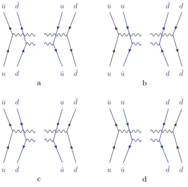
There is another type of two-parton distributions not discussed so far that do not admit a probability interpretation as they represent interference terms. Their appearance is a completely new feature compared to single hard scattering processes, where these terms are forbidden by fermion number and/or quark flavor conservation. Typical interference terms in fermion

(28)

number are

I_a₁_¯_a₂(x_i,k_i,y) =hh(¯q₂Γ_¯_a₂q₄) (¯q₃Γ_a₁q₁)ii,

I_¯_a₁_a₂(x_i,k_i,y) =hh(¯q₄Γ_a₂q₂) (¯q₁Γ_¯_a₁q₃)ii, (4.20) where the first one is displayed in figure 4.2 (d), from which can be seen that the quark in the amplitude is an antiquark in the conjugate and vice versa. Additionally, there are interference terms in quark flavor, e.g.

I_a₁_a₂(x_i,k_i,y) =hh(¯u₃Γ_a₂d₂) ¯d₄Γ_a₁u₁

ii, (4.21)

displayed in figure 4.3. In that case, the quark that is an up quark in the amplitude is a down quark in the conjugate and vice versa.

I _a

₁

_a _¯

₂

1 2 3 4

i j j^′ i^′

u d u¯ d¯

Figure 4.3.: Example for an interference distribution in quark flavor. The quark line that represents an up quark in the amplitude represents a down quark in its conjugate and vice versa.

4.1.5. Gluons

The starting point for the definition of the double gluon TMD is the two-gluon correlator Φ^j¹^j¹^′^j²^j²^′(ki, r) =

" ₂ Y

i=1

#Z d⁴y (2π)⁴e^−iyr

× hp|T¯h

A^j^′²(−¹₂z₂)A^j¹^′(y−¹₂z₁)i Th

A^j²(¹₂z₂)A^j¹(y+¹₂z₁)i

|pi . (4.22) Working in light-cone gauge,A⁺= 0, the leading contribution to the cross section originates from gluons with transverse polarization, i.e. ji, j^′_i= 1,2, but one then has to be careful about effects from Wilson lines at spacetime infinity, as the gluon potential does not vanish at infinity in light-cone gauge. Working in covariant gauges, e.g. Feynman gauge, the attachement of gluons with polarization A⁺ for the right-moving proton and of gluons with polarization A⁻ for the left-moving proton is not power suppresses and these gluons have to be resummed into appropriate Wilson lines, which we will discuss in chapter 6. After this step is taken the leading contribution to the cross section once again comes from gluons with transverse polarization and we will define the two-gluon distributions for these gluons.

For this purpose we need a decomposition of the two-gluon correlator (4.22). Any tensor