• Keine Ergebnisse gefunden

Double Parton Distributions in the Nucleon on the Lattice Dissertation

N/A
N/A
Protected

Academic year: 2021

Aktie "Double Parton Distributions in the Nucleon on the Lattice Dissertation"

Copied!
158
0
0

Wird geladen.... (Jetzt Volltext ansehen)

Volltext

(1)

Dissertation

zur Erlangung des Doktorgrades der Naturwissenschaften (Dr. rer. nat.)

der Fakultät für Physik der Universität Regensburg

vorgelegt von

Christian Zimmermann

aus Sulzbach-Rosenberg

im Jahr 2020

(2)

Prüfungsausschuss:

Vorsitzender: Prof. Dr. Dieter Weiss

Erstgutachter: Prof. Dr. Andreas Schäfer

Zweitgutachter: Prof. Dr. Markus Diehl

weiterer Prüfer: Prof. Dr. Klaus Richter

Datum Promotionskolloquium: 28.10.2020

(3)

Double Parton Distributions in the Nucleon on the Lattice

Abstract

Modern scattering experiments involving hadrons are sensitive to parton correlations, which can be parameterized by double parton distributions (DPDs). These are non- perturbative objects, which are largely unknown in theory, detailed experimental access is quite challenging. This thesis provides a first non-perturbative study from first prin- ciples of light quark DPDs in the nucleon in the framework of lattice QCD. First of all, a brief review of Quantum Chromodynamics (QCD) is given, followed by definitions and relations regarding double parton distributions. After that, the evaluation of hadronic matrix elements in the framework of lattice QCD is explained. DPDs are related to two-current matrix elements, which can be calculated on the lattice by evaluating four- point functions. We describe the corresponding Wick contractions for the case of the proton and give details on the techniques being used for their simulation. These are performed on 990 configurations of the CLS ensemble H102 with β = 3 . 4, which corre- sponds to a lattice spacing of 0 . 0856 fm, and pseudoscalar masses m π = 355 MeV and m K = 441 MeV. The data is converted to the MS scheme at a renormalization scale of µ = 2 GeV. Results of the bare Wick contractions, as well as physical combinations for specific flavor, are presented for the two-current matrix elements hV 0 V 0 i and hA 0 A 0 i , where also lattice artifacts are explored. The data of two-current matrix elements is used for the determination of twist-2 functions, which are related to the first DPD Mellin moment for a specific quark polarization. Consistence of the results with the DPD number sum rule is verified. The dependence on the quark flavor and polarization is analyzed for the twist-2 functions, as well as for the extracted DPD Mellin moments.

A further aspect to be investigated is the validity of factorization hypotheses which are

often assumed in order to decompose DPDs in terms of single parton distribution func-

tions (PDFs). This is e.g. the case in the well known pocket formula of double parton

scattering. To this end, we derive factorized expressions for hadronic matrix elements

of two operators, where we obtain convolutions of proton form factors, which can be ob-

tained from lattice calculations. We implement two versions, the corresponding results

are compared to those obtained from two-current matrix elements.

(4)
(5)

1 Introduction 1

1.1 SM background at the LHC . . . . 1

1.2 Double parton scattering . . . . 2

1.3 Outline . . . . 3

2 Hadron structure and DPDs 5 2.1 Quarks and hadron symmetries . . . . 5

2.2 Quantum chromodynamics . . . . 7

2.3 Parton correlation functions . . . 10

2.3.1 Definition . . . 10

2.3.2 Twist-2 operators . . . 13

2.3.3 GPDs and form factors . . . 15

2.3.4 Evolution . . . 17

2.4 Double parton distributions . . . 18

2.4.1 Definition for quarks . . . 18

2.4.2 Properties of collinear color-singlet DPDs . . . 20

2.4.3 Double parton scattering and DPDs . . . 22

3 Matrix elements and lattice QCD 27 3.1 The path integral formalism . . . 27

3.1.1 The concept . . . 27

3.1.2 The Wick rotation . . . 29

3.1.3 Grassmann variables and Wick’s theorem . . . 29

3.2 QCD on the lattice . . . 30

3.2.1 Discretization of the QCD action . . . 31

3.2.2 Doublers and chiral symmetry . . . 32

3.2.3 Discrete symmetries . . . 33

3.2.4 The Wilson gauge action . . . 35

3.2.5 Symanzik improvement . . . 36

3.2.6 Monte Carlo simulations and lattice QCD . . . 37

3.3 Euclidean correlation functions . . . 40

3.4 Hadronic matrix elements on the lattice . . . 41

3.4.1 Basic evaluation procedure . . . 41

3.4.2 Local operators . . . 43

3.4.3 Renormalization . . . 45

v

(6)

4 Two-current correlations in the proton on the lattice 47

4.1 Definition and properties . . . 47

4.2 Evaluation on the lattice . . . 48

4.2.1 Four-point correlation functions . . . 48

4.2.2 Wick contractions and physical matrix elements . . . 49

4.2.3 Renormalization . . . 54

4.3 Simulation details . . . 54

4.3.1 Details on the Wick contractions . . . 55

4.3.2 Lattice setup . . . 69

4.3.3 Computational details . . . 69

4.4 Results and data quality . . . 70

5 Mellin moments of DPDs 75 5.1 Relation to two-current correlations . . . 75

5.2 Twist-2 functions . . . 78

5.2.1 Data quality and artifacts . . . 78

5.2.2 Physical results for py = 0 . . . 82

5.2.3 Modeling the y 2 -dependence . . . 84

5.2.4 py -dependence and moments in ζ 2 . . . 86

5.3 Extraction of Mellin moments . . . 92

5.3.1 The model . . . 92

5.3.2 Results . . . 93

5.4 Discussion . . . 97

5.5 The number sum rule for DPDs . . . 100

6 Factorization of two-current correlations 103 6.1 Factorization approaches . . . 103

6.1.1 Factorization of skewed DPDs . . . 103

6.1.2 Factorization of local matrix elements . . . 107

6.2 The nucleon form factor . . . 108

6.2.1 Lattice calculations . . . 109

6.2.2 Properties . . . 110

6.3 Convolution results . . . 113

7 Conclusions 121 A Appendix 125 A.1 Notations and conventions . . . 125

A.2 Wick contraction symmetries . . . 128

A.3 Tensor Parameterizations . . . 128

A.4 Fourier transform h n ( x ) of polynomial terms . . . 129

A.5 Statistical analysis . . . 131

A.6 Fitting methods . . . 131

A.6.1 χ 2 minimization . . . 131

(7)

A.6.2 Linear fits and equation systems . . . 132

List of Figures 135

List of Tables 137

Acronyms 139

Bibliography 141

Acknowledgments 149

(8)
(9)

Since it has become clear in the middle of the last century that hadrons are composed of more elementary particles, the study of the hadronic structure has evolved to one of the most diverse subjects in modern particle physics. Nowadays we know that the constituents of a hadron are quarks and gluons, which are elementary particles treated by the standard model. The theory describing the dynamics and interactions between quarks and gluons is known as Quantum Chromodynamics (QCD). Hadrons can be thought of being bound states of the QCD Hamiltonian. However, the exact internal structure in terms of quarks and gluons remains unknown. While we have gained a quite reasonable understanding of some aspects, like quark and gluon distributions, there are still many open questions.

Among others, this concerns e.g. the orbital angular momentum of the hadron’s con- stituents and subsequently their contribution to the total hadron spin (proton spin puzzle) [1]. Related to this subject is the internal hadronic structure in the transverse plane in collisions with other particles. Experimental insight on these subjects should be provided by the future Electron Ion Collider (EIC) [2].

The subject being addressed by this work is the question how partons are correlated with each other in a hadron and how scattering processes are affected by these correlations.

A reasonable understanding of this is necessary for the interpretation of experiments in order to test the Standard Model (SM) or find physics beyond it, as we explain in the following.

1.1 SM background at the LHC

Thanks to their relatively large mass to charge ratio, protons can be accelerated to highest energies in circular accelerators in order to create high-energy collisions. In this context they have been used e.g. in experiments at Tevatron and nowadays are collided at the Relativistic Heavy Ion Collider (RHIC) and the Large Hadron Collider (LHC).

Therefore, hadrons play also an essential role in experiments where the validity of the standard model is explored. A prominent example is the LHC, where proton-proton col- lisions with energies up to 13 TeV are used within the four experiments ATLAS, CMS, ALICE and LHCb. Their purpose is e.g. the investigation of standard model related subjects like the experimental proof of the existence of the Higgs boson, which has been achieved in 2012 [3, 4]. Further tasks are given by the search for physics beyond the Standard Model (BSM) like dark matter physics.

BSM-particles, which are hoped to be detected in LHC experiments, have to be very

1

(10)

massive, otherwise they would have been found already. They decay into particles hav- ing much lighter masses, which leads to a very large decay phase space. However, this is also characteristic for the phase space accessible by double parton scattering (DPS) events, an interaction of the two colliding hadrons where two partons of each hadron take part. This is part of the SM background.

Among others, the production of W + W and ZZ are channels in which the Higgs bo- son has been detected in ATLAS and CMS. In both channels there may be background contributions by DPS events, e.g. double Drell-Yan (DDY) processes. Within a sim- plified and unrealistic model of the DDY process it was pointed out in the past that DDY contributions might be sufficient to describe the experimental data of W + W and ZZ production without taking into account contributions by the Higgs particle [5]. To definitely exclude such scenarios, investigations on DPS and their contribution to the SM background in LHC experiments are crucial.

1.2 Double parton scattering

The simplest parton model description of hadron-hadron interactions is given by as- suming that there is one hard parton-parton interaction, i.e. one parton of each hadron is involved. In the following, this type of interactions is referred to as single parton scattering (SPS). The corresponding cross section directly depends on the probability of finding a parton with a given longitudinal momentum, which is described by a parton distribution function. An example is the Drell-Yan (DY) process, where a quark from each of two colliding hadrons scatters, resulting in the production of a lepton-antilepton pair ( ppl ¯ l + X ) [6]. The cross section depends on the probability of finding a quark with a given fraction x of the hadron’s momentum. For a given parton a with a certain polarization this is parameterized by the corresponding parton distribution functions (PDFs) f a ( x ). Depending on the hadron, they are more or less known from experiment and lattice simulations [7, 8].

With decreasing momentum fraction x the parton density in a hadron increases. As a consequence interactions with two partons of each hadron become more probable. In particular, this is relevant at energy scales reached at the LHC. These types of interac- tion are known as double parton scattering (DPS), an example are the aforementioned DDY processes. DPS was established in pp collisions [9] and in ¯ pp collisions [10–13] a few decades ago, recent experimental observations of DPS can be found in [14–28].

However, detailed determinations of DPS contributions in experiment are challenging, since there is typically a large SPS background. A relatively clean process in this con- text has been found to be same-sign W -pair production, which is therefore a promising channel when looking for experimental DPS data [29–31].

We anticipate here the DPS cross section in terms of double parton distributions (DPDs) F ( x 1 , x 2 , y ) and the parton level cross sections σ i , which can be written as:

d σ DPS

d x 1x 1 d x 2x 2X

Z d 2 y σ 1 ( x 1 x ¯ 1 s ) σ 2 ( x 2 x ¯ 2 s ) F ( x i , y ) Fx i , y ) , (1.1)

(11)

where the sum represents contributions from all possible quark flavors, polarizations, etc.

The DPD parameterizes the probability of finding two correlated quarks at a transverse distance y and longitudinal momentum fractions x 1 and x 2 . More detailed expressions are given in chapter 2. In order to give an estimate for the size of the DPS contribution, this is often approximated by neglecting correlations in longitudinal dynamics, quark flavors and polarizations, and assuming a factorization of DPDs of the following form:

F ( x 1 , x 2 , y ) = f ( x 1 ) f ( x 2 ) T ( y ) , (1.2) where f ( x ) are PDFs and T ( y ) is a function parameterizing the dependence on the transverse quark distance. As a result one obtains a relation often referred to as the pocket formula [32]

d σ DPS

d x 1x 1 d x 2x 2 = 1 C

σ 1,SPS ( x 1 , x ¯ 1 ) σ 2,SPS ( x 2 , x ¯ 2 )

σ eff ,

σ eff := Z d 2 y ( T ( y )) 2 −1 ,

(1.3)

where σ i,SPS denote the SPS cross sections and C = 2 if the two scattering partons are the same, otherwise C = 1. The effective cross section σ eff only contains the transverse correlation of the two partons and in the simplest case is assumed to be a universal con- stant. Estimates of σ eff are given by experimental DPS studies in [9–28], where values between 1 mb and 28 mb have been found.

According to (1.1) DPS processes are sensitive to parton correlations parameterized by the DPDs. Like other kinds of parton distributions, DPDs are non-perturbative objects.

They are largely unknown. In the past there have been studies on parton correlations employing several quark models [33–39], recently also for the pion [40–43].

A non-perturbative method for calculating quantities related to DPDs from first prin- ciples is provided by Monte Carlo simulations of QCD on a Euclidean lattice. The required quark-quark correlations are obtained from evaluating local two-current ma- trix elements, which are directly related to Mellin moments in x i of DPDs:

M (n,m) ( y ) = Z d x 1 x n−1 1

Z d x 2 x m−1 2 F ( x 1 , x 2 , y ) . (1.4) The corresponding calculations have been worked out already in the past for the pion [44–46]

1.3 Outline

The purpose of this work is to study DPDs for the nucleon (in particular the proton)

within the lattice QCD (LQCD) framework. When calculating proton matrix elements

and subsequently determining the first DPD Mellin moment, we want to implement

several factorization assumptions in order to test the validity of simplifications being

(12)

employed e.g. by the pocket formula (1.3). Parts of the results presented in this work have already been published in [47].

This thesis is organized as follows: In chapter 2 we discuss subjects concerning the structure of a hadron. First of all we consider the hadronic wave function in terms of valence quarks and its symmetries and constraints w.r.t. space, flavor, spin and color.

Furthermore, we give a brief review of QCD, the fundamental theory of quark-gluon- interactions and hadron physics. After that, we introduce the factorization concept as generic description of hadrons during high-energy processes, where we introduce several kinds of parton distribution functions and discuss their meaning in certain physical con- texts. Therein we also define DPDs and describe their role in the description of double hard interactions.

In chapter 3 we continue with introducing LQCD as a non-perturbative method to eval- uate hadronic matrix elements, from which any kind of parton distribution functions can be defined. We describe the path integral formalism and the corresponding evalua- tion in discrete and finite Euclidean spacetime by employing Monte Carlo integration, a procedure, which is known as LQCD.

The matrix elements related to DPDs involve two currents and are introduced in chap- ter 4. After discussing their properties and decompositions in terms of Wick contrac- tions, we explain in detail the methods and techniques being used for the calculation of each Wick contraction in LQCD. We also list some details of the employed CLS gauge ensembles and the general setup of lattice parameters. We conclude this chapter with presenting the data for specific current insertions.

We continue in chapter 5 with explaining the relations between Mellin moments of DPDs and two-current matrix elements. The extraction of the moments includes a Fourier transformation. Because of the finite hadron momenta we have to choose some model to be able to perform the integral. We motivate our choice of the model and describe the corresponding fits on the lattice data. Finally, we present the results for the moments and check whether DPD number sum rules are fulfilled.

Chapter 6 is dedicated to exploring the validity of naive factorization assumptions which are used e.g. in the aforementioned pocket formula. We establish two approaches of fac- torizing quantities involving two-current matrix elements. Both include a convolution of nucleon form factors, which are calculated on the same lattice as the two-current matrix elements.

This thesis is summarized in chapter 7, where we give some concluding remarks and

perspectives for future research.

(13)

As already mentioned, describing the internal structure of hadrons is highly non-trivial.

Within this chapter we shall give brief introductions to various common concepts that have been established in order to describe hadron properties. A first description of the hadronic wave function in terms of (valence) quarks is provided by the quark model, which is suitable for describing certain symmetries. We shall introduce Quantum Chro- modynamics (QCD) to be able to describe the dynamics and interactions of the hadron’s constituents. The corresponding discussions can be found in standard literature [48–50].

In a scattering process hadrons can be treated as a bunch of quasi-free particles (par- tons). This assumption was first use by Bjorken and Feynman in order to explain deep inelastic scattering (DIS) and is known as parton model. In this context we shall briefly explain the concepts going into the definition and interpretation of parton distributions.

A special treatment is given to double parton distributions (DPDs), which are used in the description of double parton scattering.

2.1 Quarks and hadron symmetries

The standard model has six quark flavors and the corresponding antiquarks. They are spin-1 / 2 particles, i.e. fermions, and color charged forming a SU (3) color symmetric triplet, i.e. they couple to the strong force mediated by gluons. Together with the leptons they are grouped into three families, where the first family contains the lightest particles and the third the heaviest 1 .

The quarks of the first family, u (up, m u ≈ 2 . 2 MeV) and d (down, m d ≈ 4 . 7 MeV), have very small masses compared to the hadronic mass scale, which is about a few hundred MeV. In analogy to spin-1 / 2 states one identifies the isospin doublet ( u, d ) with the fundamental representation of the SU (2) group (often called SU (2) flavor to distinguish from other symmetries of the same group). Taking into account the s (strange, m s ≈ 95 MeV) quark, this symmetry can be extended to SU (3) flavor , which is less exact due to the heavier mass of the strange quark.

It seems natural to obtain a rough description of hadronic states by considering valance quarks coupled to multiplets w.r.t. spin, flavor and color. Since in nature one only observes color neutral states, i.e. color singlets (see discussion in section 2.2), hadrons have to be built from the combinations q q ¯ (mesons) and qqq (baryons), where the latter has to be totally antisymmetric in color.

Considering SU (2), which is the symmetry group of spin and flavor, and taking into

1 In this statement we neglect the neutrinos, where each one has a mass smaller than 2 eV.

5

(14)

account only u and d quarks, the mesons are decomposed in following multiplets:

2 ⊗ ¯2 = 3 ⊕ 1 , (2.1)

i.e. a triplet with (iso)spin 1 and a singlet with (iso)spin 0. Examples for the isospin- triplet are the pions (spin 0) and rho-mesons (spin 1). The flavor symmetry leads to very similar properties of the particles belonging to the same multiplet, e.g. their masses.

Discrepancies can be explained with different masses and electric charges of the quarks.

The breaking of the symmetry becomes more relevant if we consider SU (3) flavor , where the mesons decompose into an octet and a singlet:

3 ⊗ ¯3 = 8 ⊕ 1 , (2.2)

where the mass spectrum of the octet strongly depends on strangeness, i.e. the number of strange quarks in the leading Fock state of the corresponding particles. Notice that the SU (2) flavor -triplet is contained in the octet. Since the flavor symmetry is not exact, the corresponding singlet state turns out to mix with an octet state having the same quantum numbers, which results in the spin-0 mesons η and η 0 .

For baryons the situation is more involved. The total wave function has the structure

| baryon i = | space i ⊗ | flavor i ⊗ | spin i ⊗ | color i , (2.3) and has to be totally antisymmetric against permutation of quarks. In the ground state, where there is no orbital angular momentum, | space i has to be symmetric ( s -waves) and

| color i must be antisymmetric in order to obtain a color singlet. This implies that only symmetric combinations of | flavor i ⊗ | spin i are present in nature. The spins are coupled to spin-1 / 2 (mixed symmetry) or spin-3 / 2 (symmetric) states. Again considering the symmetry groups SU (2) (spin, flavor) and/or SU (3) flavor we obtain:

2 ⊗ 2 ⊗ 2 = 4 S ⊕ 2 M ⊕ 2 M ,

3 ⊗ 3 ⊗ 3 = 10 S ⊕ 8 M ⊕ 8 M ⊕ 1 A , (2.4) where the subscripts S (symmetric), M (mixed) and A (antisymmetric) label the sym- metry of the corresponding states. Since the SU (3)-singlet is antisymmetric and there is no antisymmetric spin wave function, it does not occur in nature.

Nucleons, i.e. the proton and the neutron, are spin-1/2 particles, hence their flavor part

can be written in terms of SU (2)-doublet ( I = 1 / 2) or SU (3)-octet states, such that

the overall spin-flavor wave function is symmetric. Notice that within this thesis we do

not consider effects caused by electromagnetism and always assume that u and d quarks

have the same mass, i.e. we consider an exact flavor symmetry of the group SU (2) flavor .

Hence, the results obtained for the proton can be mapped onto the neutron case by

suitable symmetry operations. Omitting permutations of the quark spins, the proton

(15)

wave function can be written as:

|p i = √ 1 6

h |u u d i + |u u d i − 2 |u u d i i . (2.5) The description given so far takes into account only the simplest Fock state in each case and does neither give any information about spatial distributions or correlations of quarks in a hadron nor about its internal dynamics. Before we continue with more sophisticated descriptions of hadrons, it is necessary to discuss the dynamics and inter- actions of the hadron’s constituents, i.e. quarks and gluons, which we do in the following section.

2.2 Quantum chromodynamics

In the following, we want to give a review of the fundamental theory of hadron physics, which is known as Quantum Chromodynamics (QCD). It provides a description of the dynamics and interactions of color charged particles, in particular the hadron’s con- stituents, i.e. quarks and gluons. Like for other gauge theories one considers invariance of the physical system under a certain kind of local gauge transformations. As men- tioned in the previous section, the gauge group of QCD is SU (3), which is a non-Abelian group.

We start with considering free Dirac fermions with mass m , which are described by the Dirac equation:

( i∂ /m ) ψ ( x ) = 0 , (2.6)

with / = γ µ µ . The Dirac matrices γ µ are elements of the Clifford algebra {γ µ , γ µ } = 2 g µν . The solutions ψ are plane waves

ψ ( x ) =

u λ ( p ) e −ixp

v λ ( p ) e +ixp , (2.7)

where u and v are Dirac spinors, which transform in a four dimensional representation of the Lorentz group. Therefore, the description is already relativistic. There are two types of spinor solutions, which are denoted by u λ ( p ) (particles) and v λ ( p ) (antiparticles), where λ labels the quark helicity. These solutions fulfill the completeness relations:

X

λ

u λ u ¯ λ = / p + m ,

X

λ

v λ v ¯ λ = p /m , (2.8)

where ¯ . denotes Dirac conjugation, which is defined by ¯ ψ = ψ γ 0 for a given Dirac spinor

ψ , such that the product ¯ ψψ is a Lorentz scalar.

(16)

The Dirac field is quantized by imposing anti-commutation relations, which are usually supposed to be fulfilled at equal time:

n ψ ˆ ( x ) , ψ ˆ ( y ) o x

0

=y

0

= δ (3) ( ~x~y ) ,

n ψ ˆ ( x ) , ψ ˆ ( y ) o x

0

=y

0

= n ψ ˆ ( x ) , ψ ˆ ( y ) o x

0

=y

0

= 0 . (2.9) The operator ˆ ψ is understood to annihilate a particle and create an antiparticle, whereas ψ ˆ¯ creates a particle and annihilates an antiparticle. Throughout this work, we consider quarks, the corresponding operators are denoted by q and ¯ q . Within the parton model, which will be introduced in the following section, the fields are considered to be quan- tized in an alternative way. The anti-commutation relations (2.9) are modified such that they are fulfilled at equal light-cone time x + = ( x 0 + x 3 ) /

2 = y + = ( y 0 + y 3 ) / √ This is known as light-cone or light-front quantization [51]. 2.

The Lagrangian being connected to (2.6) via the Euler-Lagrange equation reads:

L free ( x ) = ¯ ψ ( x ) ( i∂ /m ) ψ ( x ) . (2.10) As mentioned before, we require the theory to be invariant under local SU (3) trans- formations. The spinor fields ψ are considered to transform in the three-dimensional fundamental representation of SU (3), i.e. :

ψ ( x ) → Ω( x ) ψ ( x ) ,

ψ ¯ ( x ) → ψ ¯ ( x ) Ω ( x ) , (2.11) where we define the local gauge transformation Ω( x ) as:

Ω( x ) = e

j

(x)t

j

, (2.12)

with eight position dependent parameters θ j ( x ) and the generators t j of SU (3), which obey:

h t j , t k i = if jkl t l . (2.13) Usually one chooses the Gell-Mann basis for t j . The constants f jkl are called structure constants of SU (3), which are totally anti-symmetric under permutations of their in- dices.

While the mass term in (2.10) is trivially invariant under Ω( x ), we obtain an additional term −t j j arising from the derivative on the local transformation. To restore gauge invariance we have to extend the derivative in a gauge covariant manner:

D µ ( x ) := µig 0 A j µ ( x ) t j , (2.14)

(17)

where we have introduced a second kind of fields, the gauge fields A j µ called gluons. They transform in the adjoint representation of SU (3) and are by construction of dimension length −1 :

t j A j µ ( x ) → Ω( x ) t j A j µ ( x ) + ig 0 −1 µ ( x ) . (2.15) g 0 is the (bare) coupling constant. A consequence of the replacement by the covariant derivative (2.14) in (2.10) is the interaction of the fermions with the gauge fields, which is tuned by the coupling constant g 0 .

To complete the theory, we also need to describe the free propagation of the gauge fields themselves, i.e. we have to construct a Lorentz and gauge invariant expression of dimension length 4 only built out of these fields. A suitable quantity is:

L G ( x ) = − 1

4 F µν j ( x ) F jµν ( x ) , (2.16) with the field strength tensor

F µν j ( x ) := µ A j ν ( x ) − ν A j µ ( x ) + g 0 f jkl A k µ ( x ) A l ν ( x ) . (2.17) A fundamental difference to the electromagnetic field strength is that the last term, which arises from the non-Abelian property of SU (3), includes self-interaction between the gluons. Adding (2.16) to the gauge covariant form of (2.10) and taking into account n f quark flavors labeled by the index f , we finally obtain the Lagrangian of QCD:

L QCD ( x ) = X

f

ψ ¯ f ( x ) ( iD /m f ) ψ f ( x ) − 1

4 F jµν ( x ) F µν j ( x ) . (2.18) Performing perturbative calculations to a given order of α s = g 0 2 / (4 π ), one will encounter divergences resulting from loop integrals, which have to be regularized in a suitable scheme. The essence is to isolate the divergent terms, which can be tuned by a regulator, and re-define the constants of the theory, e.g. the quark masses m q or the coupling g 0 , such that everything remains finite, once the regulator is removed. This is known as renormalization. Notice that this introduces a renormalization scale µ the constants subsequently depend on.

In the case of QCD (and similar for all non-Abelian gauge theories) one finds that the renormalized coupling α s ( µ ) reads at 1-loop order:

g 0 2

4 π = α s Renormalization

−−−−−−−−−→ α s ( µ ) = 2 π

11 − 2 3 n f log Λ −1 QCD µ , (2.19)

with the mass scale Λ QCD , where the coupling diverges. This is often referred to as the

soft energy scale. Quantities involving this region of strong coupling cannot be calcu-

lated perturbatively. A non-perturbative method, LQCD, is described in chapter 3. In

the strong coupling limit one can derive a linear potential between color charged parti-

(18)

cles, which is responsible for the phenomenon of confinement, i.e. color charged particles are always bound in a color singlet. On the other hand, in the limit of infinitely large energies or momentum transfers the coupling goes to zero. Therefore, color charged particles are asymptotically free at large scales, such that hard scattering processes, e.g.

between quarks, are accessible by perturbation theory.

2.3 Parton correlation functions

Within the parton model, hadrons are treated as a cluster of quasi-free particles called partons. A hadronic scattering process is then described by an interaction of one or more partons with the scattering counter part. Within this scheme the process is separated into a hard process at parton level and a soft part concerning the hadronic structure. The hard process involves a high energy scale, which according to (2.19) allows a perturbative treatment.

In the following, we focus on the soft part, which is described by so-called parton correlation functions. These are non-perturbative objects and describe the appearance of partons with certain properties in a specific hadron. Throughout this work, we consider (anti)quarks. Gluons can be treated in an analogue way. For reviews on subjects regarding parton correlation functions and various types of parton distributions, as well as their interpretation, see [52, 53].

2.3.1 Definition

Within a typical scattering experiment hadrons are accelerated to very high energies

Q , which are much larger than the hadronic mass scale Λ, i.e. Λ Q . Therefore, the hadron’s four-momentum may be considered as almost light-like. Assuming that the hadron moves in 3-direction, we can express the momentum in light-cone coordinates p = ( p + , p , p ) (see also (A.13) for the notation), where

p +Q , p ∼ Λ 2

Q , p = 0 . (2.20)

p denotes the transverse vector components p = ( p 1 , p 2 ). In this scenario a hadron turns into a flat bunch of partons due to Lorentz contraction. Time dilatation causes the system to be nearly frozen, i.e. the partons can be seen as quasi-free particles with momentum k = ( k + , k , k ), with k +p + and k p . k + can be expressed by the longitudinal momentum fraction x , which indicates how much of the hadron’s momentum is carried by the parton:

k + = xp + . (2.21)

(19)

k− 2 k + 2 x + ξ x−ξ

2 2

1+ ξ 1 −ξ

x + ξx + ξ

1+ ξ 1 −ξ

Figure 2.1: Diagrammatic illustration of a parton correlation function. The blue blob represents the hadron from which the quarks emerge. For the quarks and the hadron we indicate the corresponding momenta, where the longitudinal momenta are given in terms of the fraction w.r.t. p + . The l.h.s. shows the situation if x + ξ , as well as xξ , is positive. The change of sign of one fraction turns the corresponding quark in the wave function to an antiquark in its complex conjugate and vice versa. For xξ < 0 this is shown on the r.h.s. .

If the spectator partons are considered to be on mass shell, momentum conservation yields the constraint 0 < x < 1. The transverse parton momenta are considered to be small, at most at the hadronic mass scale. In total we have the relations:

k ∼ Λ 2

Q , |k| ∼ Λ . (2.22)

With this setup we define the parton correlation function Φ αβcd ( x, k, ξ, ) := Z d 2 z d z

(2 π ) 3 e ixp

+

z

e −ikz

× hp + ∆ / 2 | q ¯ αc ( −z/ 2) q βd ( z/ 2) |p − ∆ / 2 i| z

+

=0 .

(2.23)

The initial and the final hadron state are parameterized symmetrically in terms of the momentum variables p and ∆. The two quark operators in (2.23), which are considered to be light-cone quantized, are evaluated at z + = 0, i.e. at equal light-cone time. This is equivalent to integrating over − -components of the quark momenta, such that the quarks created or annihilated by q and ¯ q are not on mass shell. Furthermore, the quark operators anti-commute, which can be seen as an implementation of the quasi- free partons considered within the parton model.

By considering the Fourier expansion of the light-cone quantized quark field q , we see

that depending on the sign of the +-momentum it removes a quark from the hadron

wave function or creates an antiquark in its complex conjugate. An analogue behavior is

found for ¯ q . If all quark +-momenta are positive, this can be interpreted as the emission

of a quark with momentum k − ∆ / 2 and the absorption of a quark with momentum

k +∆ / 2. A changing sign in the +-momentum turns the quark in the wave function into

an antiquark in the complex conjugate wave function and vice versa. This is depicted

in Figure 2.1. The dependence on the longitudinal momentum change is parameterized

(20)

in terms of the fraction ξ w.r.t. p + :

ξ = − ∆ +

2 p + . (2.24)

There are two kinds of processes which can be described by parton correlation functions.

The first one is called (semi-)inclusive, which means that only a part of the scattering products is actually detected. The cross section involves matrix elements hX| q |pi de- scribing the emission of a quark leaving a set of spectator partons which are not resolved in the measurement. They have to be included in the squared amplitude by a sum over all possible final states. Roughly sketched, the hadronic part of the squared amplitude has then the form P X hp| q ¯ |Xi hX| q |pi . This is what we get if we insert a complete set of states in the matrix element appearing in (2.23) for ∆ = 0. On the other hand we consider exclusive processes with only the scattered hadron in the final state. In this case the amplitude involves hadronic matrix elements of the form hp| T¯ qq |p 0 i , where T denotes time ordering. The matrix element describes the emission of a quark and the subsequent absorption leading to a total momentum change ∆ = p− p 0 . It can be shown that the time ordering may be dropped if ¯ q and q are evaluated at equal light-cone time [54]. Again, the matrix element can be identified with (2.23).

The concept of quark correlation functions can be extended to n quarks, see [55]. With the additional average quark momenta k i this introduces further degrees of freedom given by the differences r i between the quark momenta. Within the chosen frame the introduced parton momenta scale similarly to (2.22):

p +k i +r i +Q , p k i r i ∼ Λ 2

Q k ir i ∼ Λ .

(2.25)

Since we shall only consider such correlation functions to represent the squared ampli- tude in the cross section, it is sufficient to consider ∆ = 0. The n -parton correlation function for quarks can be defined as:

Φ α

i

β

i

c

i

d

i

( x i , k i , ζ i , r i ) = (2 p + ) n−1

×

"

Y

i

Z d 2 z i d z i

(2 π ) 3 d 2 y i d y i e ix

i

p

+

z

i

e −ik

i

z

i

e −iζ

i

p

+

y

i

e ir

i

y

i

#

δ ( y n ) δ (2) ( y n )

× hp| Y

i

¯

q i,c

i

α

i

( y iz i / 2) q i,d

i

β

i

( y i + z i / 2) |pi

z

+i

=0

y

+i

=0

.

(2.26)

The quark momentum difference r i is the Fourier conjugate variable to the average

quark position y i . Again we parameterize its longitudinal component as fraction w.r.t.

(21)

k 1 + r 2

1

k n + r 2

n

k nr 2

n

k 1r 2

1

z

1

2 y n + z 2

n

y nz 2

n

z 2

1

. . . . . .

p p

Figure 2.2: Depiction of a n -parton correlation function. The blue blob represents the hadron emitting and absorbing n partons. For each parton we show the corresponding momentum. Under the assumption that r i is the Fourier conjugate variable to y i and y n = 0 we can assign r n = − P n−1 i=1 r i .

total hadron momentum p + :

ζ i = r + i

p + . (2.27)

We are free to choose y n = 0 because of translational invariance, i.e. y i , with i 6 = n can be seen as the average distance to the n -th parton. Subsequently, only n − 1 of the momentum variables r i are independent. In the following we set r n = − P n−1 i=1 r i . The structure of the correlation function in terms of the involved momenta is depicted in Figure 2.2.

2.3.2 Twist-2 operators

Contracting (2.23) or (2.26) with Γ αβ , where Γ is a suitable Dirac matrix, selects a certain quark polarization. A further contraction with a Kronecker delta δ cd couples the corresponding quark fields to a color singlet. For the general n -parton correlation function (2.26) there are further possibilities for selecting different color representations as we will see when we discuss DPDs. The contracted operator ¯ q Γ q is classified by a number called twist, which was originally defined through the suppression by mass terms after applying the operator product expansion (OPE). In the present case we are interested in leading twist, i.e. twist 2, the corresponding operators are those with a maximal number of plus components. Matrix elements of these operators are most relevant, since by Lorentz invariance they scale with p + , which is considered to be large.

Furthermore, twist-2 operators represent only dynamically independent ("good") light-

cone components of the quark fields, which allows a probabilistic interpretation within

the parton model. For a detailed discussion on that we refer to [56]. There are three

types of twist-2 operators, which correspond to the polarization of the quark. They

can be constructed from helicity projection operators, γ + (1 ± γ 5 ) / 2 or the projection

operator for transverse spin s j , which is ( γ + ± s j j+ γ 5 ) / 2. For flavor q the twist-2

(22)

operators labeled by a = q,q, δq are:

O a ( y, z ) := ¯ q ( yz/ 2) Γ a q ( y + z/ 2) | z

+

=0 , (2.28) with

Γ q = 1

2 γ + unpolarized quark , Γ ∆q = 1

2 γ + γ 5 longitudinal polarization , Γ j δq = i

2 σ j+ γ 5 transverse polarization .

(2.29)

The ⊥ -notation is introduced to distinguish between the operators (2.28) and those that are defined for vanishing transverse quark distance. These kind of operators we shall introduce later in this work. The operators (2.28) can be related to their analogue for antiquarks by considering charge conjugation C , where we find:

O ¯ a ( y, z ) := O ⊥,C a ( y, z ) = ¯ q ( y + z/ 2) Γ ¯ a q ( yz/ 2) | z

+

=0 = η a C O a ( y, −z ) , (2.30) such that

Γ ¯ a = η C a Γ a , (2.31)

where the sign factors η C a depend on the channel:

η C a =

1 a = ∆ q

− 1 a = q, δq . (2.32)

Notice that the operators (2.28) and (2.30) are not invariant under local gauge trans- formations, since the quark fields are evaluated at different positions. In order to keep everything gauge invariant, it is necessary to introduce Wilson lines between the quark fields, i.e.

q ( z ) → q W ( z, v ) := W ( z, v ) q ( z ) . (2.33) The Wilson lines W ( z, v ) represent collinear gluons and their explicit shape is specific to the considered process. For a detailed discussion see [57] and in the context of multi parton interactions [55]. For semi-inclusive DIS (SIDIS) and DY one finds

W ( z, v ) = P exp ±ig

Z ∞

0 d η v t j A j ( zηv ) , (2.34)

where v is a space-like vector and P denotes path ordering. The two possible signs in

(2.34) are specific to the process and correspond to future (SIDIS) and past (DY,DDY)

pointing Wilson lines.

(23)

2.3.3 GPDs and form factors

In the following, we consider correlation functions involving a single light-cone quark operator. In addition to the integral over k we also integrate out the transverse quark momentum with the results that there is no sensitivity to transverse dynamics in the hadron. The resulting quantity is called generalized parton distribution (GPD). For reviews on subjects concerning GPDs, see [58, 59], where in the latter the term off- forward parton distribution (OFPD) is used. The GPD is defined as:

f a ( x, ξ, t ) := (Γ a ) αβ δ cd

Z d 2 k Φ αβcd ( x, k, ξ, ∆)

= Z d z

2 π e ixp

+

z

hp + ∆ / 2 | O a (0 , z ) |p − ∆ / 2 i ,

(2.35)

with

O a ( y, z ) := ¯ q ( yz/ 2)Γ a q ( y + z/ 2) | z

+

=0,z=0 . (2.36) Again Γ a selects the quark polarization. Note that in the case z = 0 the Wilson lines are just straight gauge links between the quark fields. In light cone gauge A + = 0 the links become trivial. As mentioned in the previous section, GPDs enter the calculations for the cross sections of exclusive scattering processes like deeply virtual Compton scattering (DVCS). For particles with zero spin or after taking the spin average, it can be shown that by Lorentz invariance the GPDs only depend on the following variables [58]:

x = k +

p + , ξ = − ∆ + 2 p + , t = ∆ 2 = − 4 ξ 2 m 2 + 2

1 − ξ 2 .

(2.37)

As already discussed, emitted quarks with negative +-momentum are interpreted as absorbed antiquarks. Therefore, it depends on the sign of xξ ( x + ξ ) whether a quark is emitted (absorbed) or an antiquark absorbed (emitted). Notice that the momen- tum fraction is restricted by |x| < 1. Otherwise momentum conservation would imply spectator partons with negative +-momentum. However, this is not possible, since the spectator partons are considered to be on mass shell.

For spin-1/2 particles like the nucleon we have an additional quantum number charac- terizing the initial and final state, which is the helicity λ , i.e. the longitudinal hadron polarization. The corresponding GPD matrix elements f λλ

0

depend on , i.e. not only on t . They can be parameterized in terms of two independent functions, as we will discuss later.

If we consider a GPD for ∆ = 0, we obtain a simple parton distribution function (PDF)

f a ( x ) = f a ( x, ξ = 0 , t = 0) , (2.38)

(24)

which yields the probability to find a parton with longitudinal momentum xp + and polarization a . As mentioned in the previous section, the cross sections of inclusive processes like DIS can be written in terms of PDFs.

GPDs are related to form factors F a ( t ), which can be identified with a Fourier transform of the charge density in the transverse plane in the infinite momentum frame [60]. More precisely, it is the first Mellin moment in x of a GPD. The n -th Mellin moment is defined by

F a (n) ( ξ, t ) := Z 1

−1 d x x n−1 f a ( x, ξ, t ) . (2.39) In the case of n = 1, which is equivalent to integrating the GPD over x , we find that the Mellin moment is independent of ξ , which is a consequence of Lorentz invariance:

F a (1) ( ξ, t ) = F a ( t ) := Z 1

−1 d x f a ( x, ξ, t ) . (2.40) Higher Mellin moments F (n) ( ξ, t ) in general decompose into an even polynomial in ξ of at most n -th degree. The corresponding coefficients, which depend on t , are called generalized form factors (GFFs). Integrating over x yields a delta function in z , which fixes z to zero. Therefore, the form factor can be defined by the hadronic matrix element of a local quark current.

p + F a ( t ) = hp + ∆ / 2 | q ¯ (0) Γ a q (0) |p − ∆ / 2 i . (2.41) Replacing +-components by a Lorentz index, this equation can be brought into a Lorentz covariant form.

Let us now consider hadrons having non-zero total spin, which is the case for all baryons.

In the following, we want to consider spin-1 / 2 hadrons, like the nucleon. The corre- sponding hadron states are classified by an additional quantum number referring to the longitudinal hadron spin (helicity) λ = ± 1 / 2. Since spin-1 / 2 particles are represented by Dirac spinors, matrix elements of an operator O can be expressed in terms of Dirac spinors and a specific decomposition J [ O ] of the operator:

hp + ∆ / 2 , λ| O |p − ∆ / 2 , λ 0 i = ¯ u λ ( p + ∆ / 2) J [ O ] u λ

0

( p − ∆ / 2) . (2.42) Explicit expressions for the decomposition J [ O ] follow from Lorentz symmetry. This is discussed e.g. in [59]. In the following, we concentrate on the cases of vector currents

¯

µ q and axial vector currents ¯ µ γ 5 q . For these currents a decomposition is given by:

J [¯ µ q ] = F 1 ( t ) γ µ + F 2 ( t ) µνν

2 m , J [¯ µ γ 5 q ] = g A ( t ) γ µ γ 5 + g P ( t ) γ 5 ∆ µ

2 m .

(2.43)

(25)

For each channel there are two independent form factors, in the vector case F 1 , F 2 and in the axial vector case g A and g P (depending on the literature the latter is also denoted by g P ˜ ). At t = 0, P q e q F 1 q and P q e q F 2 q correspond to the hadron charge and the anomalous magnetic moment, respectively

The extension of the GPD (2.35) to spin-1 / 2 hadrons works analogously to that of the form factors. Here one finds the following parameterization [58]:

f a λλ

0

( x, ξ, ) = Z d z

2 π e ixp

+

z

hp + ∆ / 2 , λ| O a (0 , z ) |p − ∆ / 2 , λ 0 i

= 1

2 p + u ¯ λ ( p + ∆ / 2) J a ( x, ∆) u λ

0

( p − ∆ / 2) ,

(2.44)

with

J q ( x, ∆) = H q ( x, ξ, t ) γ + + E q ( x, ξ, t ) +jj

2 m , J ∆q ( x, ∆) = ˜ H q ( x, ξ, t ) γ + γ 5 + ˜ E q ( x, ξ, t ) γ 5+

2 m .

(2.45)

In analogy to (2.40) the form factors F 1 , F 2 , g A and g P can be identified as Mellin moments of the GPDs H , E , ˜ H and ˜ E

F 1 ( t ) = Z d x H ( x, ξ, t ) , F 2 ( t ) = Z d x E ( x, ξ, t ) , g A ( t ) = Z d x H ˜ ( x, ξ, t ) , g P ( t ) = Z d x E ˜ ( x, ξ, t ) .

(2.46)

2.3.4 Evolution

The matrix elements appearing in (2.23) and (2.26) involve so-called rapidity diver- gences. These are removed in the collinear case, i.e. by integrating over transverse momenta, however, this causes divergences due to infinitely large transverse parton mo- menta, i.e. ultraviolet divergences. Both kinds of divergences require an appropriate regularization and renormalization procedure. As a consequence the distribution func- tions we considered so far depend on the renormalization scale µ and (in the transverse momentum dependent (TMD) case) on rapidity cut-off parameters. The dependence on these parameters and the scale is referred to as evolution and is describe by the Dokshitzer Gribow Lipatow Altarelli Parisi (DGLAP) equations in the collinear case or by Collins-Soper evolution in the TMD case.

Considering e.g. the GPDs (2.35), where we have collinear evolution, the corresponding dependence on the scale µ is described by the differential equation:

log µ f a ( x, ξ, t ; µ ) = X

a

0

Z 1

−1 d x 0 P aa

0

( x, x 0 , ξ, α s ( µ )) f a

0

( x 0 , ξ, t ; µ ) , (2.47)

(26)

which is a generalization of the DGLAP equation for PDFs. The functions P aa

0

are called evolution kernels.

2.4 Double parton distributions

Now we want to give definitions and relations regarding the DPDs, which are the ob- jects we want to investigate in this work. We shall focus on DPDs of quarks only.

Furthermore, we only assume the unpolarized case, i.e. hadrons with spin zero or the spin average.

2.4.1 Definition for quarks

DPDs are given by the k -integrated 2-parton correlation function. In the following, we concentrate on quark distributions and the corresponding spin structure, again only considering color singlet operators. The corresponding DPD 1 F is obtained from (2.26), considering n = 2:

1 F ab ( x i , k i , ζ, y ) = (Γ a ) α

1

β

1

b ) α

2

β

2

δ c

1

d

1

δ c

2

d

2

Z d 2 r

(2 π ) 2 e −iyr Φ α

i

β

i

c

i

d

i

( x i , k i , ζ, r )

= 2 p +

Z d y e −iζp

+

y

 Y

i=1,2

d 2 z i d z i

(2 π ) 3 e ix

i

p

+

z

i

e −iz

i

k

i

× hp| O a ( y, z 1 ) O b (0 , z 2 ) |pi

y

+

=0 ,

(2.48)

where ζ is defined as:

ζ = r +

p + . (2.49)

In contrast to one-parton distributions the quark bilinears can be coupled to a color- octet, the corresponding DPD is denoted by 8 F . It is obtained by replacing the Kro- necker deltas δ c

i

d

i

by a sum over Gell-Man matrices t a c

1

d

1

t a c

2

d

2

. From now on we restrict ourselves to the color-singlet DPDs 1 F and drop the index 1 for simplicity.

Interchanging the spinor and color indices such that (Γ a ) α

1

β

1

b ) α

2

β

2

δ c

1

d

1

δ c

2

d

2

→ (Γ a ) α

1

β

2

b ) α

2

β

1

δ c

1

d

2

δ c

2

d

1

yields distribution functions corresponding to fermion num- ber interference. This is not discussed in detail within this work.

If ζ 6 = 0, the DPD is called non-forward or skewed, meaning that the emitted quarks have different longitudinal momenta than the absorbed ones. Within the DPS phe- nomenology this case is not relevant, as is discussed later in this section.

F ab is related to the probability of finding two quarks of polarization a and b simulta-

neously. Since the transverse quark momenta k i and the transverse distance y cannot

be measured at the same time due to the uncertainty principle, the DPDs we defined

above do not have a direct probabilistic interpretation. However, integrating over the

Abbildung

Figure 2.5: Support region for the skewed DPD F ud ( x 1 , x 2 , ζ, y ) for − 1 ≤ ζ ≤ 0 (left) and 0 ≤ ζ ≤ 1 (right) in the ( x 1 , x 2 )-plane
Figure 3.2: The clover term Q µν ( x ) (left) and the rectangle ˜ U µν ( x ) (right), shown in the ( µ, ν )-plane
Figure 4.4: Contributions to hp| O uu i (0) O j dd ( y ) |pi with C 1 topology. The forward prop- prop-agator M z is depicted by a simple line, the stochastic propagator ψ by a zigzag line and the sequential propagator X (without the incorporated forward p
Figure 4.5: Same as Figure 4.4 showing the contributions to hp| O uu i (0) O uu j ( y ) |pi with C 1 topology.
+7

Referenzen

ÄHNLICHE DOKUMENTE

In this paper, we carry out the first direct lattice calculation for the valence quark distribution of the pion using the LaMET approach.. Our results are comparable quantitatively

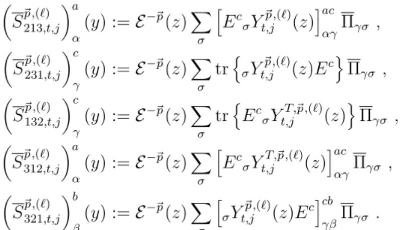
APPENDIX B: OPERATOR RELATIONS FOR LEADING-TWIST DISTRIBUTION AMPLITUDES In the following we give the relations between the operators whose matrix elements dene moments of the

The nucleon distribution amplitude can be inferred from matrix elements of local three-quark operators, and a central issue in our approach is the renormalization these operators..

ner (formed from the sar by prefixing J „the 60th part&#34;), the word would be Assyrian and mean ,,r yoke&#34;, while the Accadian representative was su¬. tu 1 or sudun. The ner

The tree-level production modes of a vector boson in association with jets

quantum chromodynamics (QCD), while providing constraints on the quark distributions in a similar way to inclusive production of a vector boson. The PDF fit is performed at NNLO

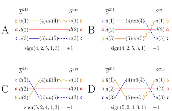
Combining the different lattice graphs to physical amplitudes in an isospin basis, we can compare our lattice results with the computation in chiral perturbation theory performed

LHCb VELO data event 2d projection, top half 37 Daniel Saunders, iCSC 2016 - Data Reconstruction in Modern Particle Physics Lecture 1/2... Tracking - Pattern recognition Tracking