Two-current correlations in the pion on the lattice

JHEP12(2018)061

Published for SISSA by Springer

Received : August 1, 2018 Revised : November 6, 2018 Accepted : November 22, 2018 Published : December 11, 2018

Two-current correlations in the pion on the lattice

Gunnar S. Bali,

Peter C. Bruns,

Luca Castagnini,

Markus Diehl,

Jonathan R. Gaunt,

Benjamin Gl¨ aßle,

Andreas Sch¨ afer,

Andr´ e Sternbeck

and Christian Zimmermann

a

Institute for Theoretical Physics, University of Regensburg, 93040 Regensburg, Germany

b

Department of Theoretical Physics, Tata Institute of Fundamental Research, Homi Bhabha Road, Mumbai 400005, India

c

Nuclear Physics Institute, Academy of Sciences of the Czech Republic, Hlavni 130, 25069 ˇ Reˇ z, Czech Republic

d

Fachbereich Physik, University of Hamburg, Jungiusstraße 9-11, 20355 Hamburg, Germany

e

Deutsches Elektronen-Synchroton DESY, Notkestrasse 85, 22607 Hamburg, Germany

f

Theoretical Physics Department, CERN, CH-1211 Geneva 23, Switzerland

g

Zentrum f¨ ur Datenverarbeitung, Universit¨ at T¨ ubingen, W¨ achterstr. 76, 72074 T¨ ubingen, Germany

h

Theoretisch-Physikalisches Institut, Friedrich-Schiller-Universit¨ at Jena, Max-Wien-Platz 1, 07743 Jena, Germany

E-mail: gunnar.bali@ur.de, bruns@ujf.cas.cz, markus.diehl@desy.de, jonathan.richard.gaunt@cern.ch, benjamin.glaessle@ur.de,

andreas.schaefer@ur.de, andre.sternbeck@uni-jena.de, christian.zimmermann@ur.de

Abstract: We perform a systematic study of the correlation functions of two quark cur- rents in a pion using lattice QCD. We obtain good signals for all but one of the relevant Wick contractions of quark fields. We investigate the quark mass dependence of our results and test the importance of correlations between the quark and the antiquark in the pion.

Our lattice data are compared with predictions from chiral perturbation theory.

Keywords: Lattice QCD, Chiral Lagrangians

ArXiv ePrint: 1807.03073

JHEP12(2018)061

Contents

1 Introduction 1

2 Correlation functions of two currents 3

2.1 Isospin decomposition and constraints 4

2.2 Predictions from chiral perturbation theory 5

3 Lattice techniques 7

3.1 Lattice contractions and their symmetry properties 7

3.2 Physical matrix elements 8

3.3 Simulation details 11

3.4 Renormalisation 17

4 Data quality and lattice artefacts 19

4.1 Plateaux and excited state contributions 19

4.2 Anisotropy effects 20

4.3 Finite volume effects 22

4.4 Finite momentum and boost invariance 23

5 Results for individual lattice contractions 25

5.1 Light quarks 26

5.2 Quark mass dependence 27

5.3 Test of factorisation 28

5.4 Root mean square radii 32

5.5 Subtraction term for the annihilation graph 37

6 Results for isospin amplitudes 38

6.1 Isospin amplitudes 38

6.2 Comparison with chiral perturbation theory 41

7 Summary 42

1 Introduction

The study of hadronic form factors has a long history in QCD and remains an active

field of study. Defined from the matrix elements of single currents, form factors contain

information about the spatial distribution of charge inside a hadron. Going beyond this,

the matrix elements of two currents at different points in space are sensitive to charge

correlations and thus yield qualitatively new information about QCD bound states and

their many-body structure.

JHEP12(2018)061

Hadronic matrix elements of one or two currents can be calculated in lattice QCD. In fact, it was realised long ago that two-current correlators on the lattice can be regarded as gauge invariant probes of hadron wave functions. Following earlier work [1–8], detailed computations for the vector, scalar and pseudoscalar currents were presented in [9, 10] and extended studies for the vector current in [11]. These studies focused on a broad range of physics and observables, such as confinement [1, 2], the size of hadrons [3–5, 8], comparison with quark models [7], or the non-spherical shape of hadrons with spin 1 or larger [9–11].

The computation of two-current correlators on the lattice involves many different Wick contractions of the quark fields, including disconnected graphs and graphs with all-to-all propagators. This presents major challenges, for the sheer amount of calculations and for obtaining statistically significant results. Whilst the work in [1–11] focused on the graph denoted by C

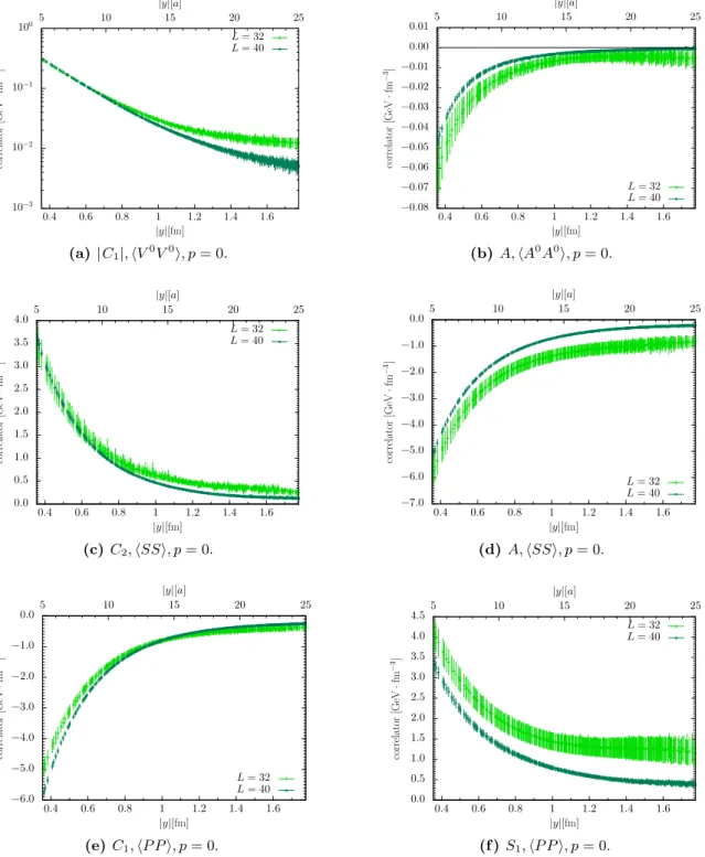
in figure 2, we study all relevant contractions for a meson here (leaving the case of baryons for future work). We also extend the set of currents mentioned above by the axial current. Last but not least, increased computing power has allowed us to use larger lattices and a smaller pion mass than previous studies. Indeed, we will see that finite volume effects can be appreciable for the quantities we are interested in.

At large distances between the two currents, the correlation functions we consider can be evaluated in chiral perturbation theory, which describes the low-energy limit of QCD in terms of mesons and their interactions. A leading-order calculation, supplemented by an estimate of higher orders using resonance exchange graphs, has been performed in [12], and we will compare our lattice results with these predictions.

An extension of the work presented here allows us to compute matrix elements that, as explained in [13], can be connected with the Mellin moments of double parton distributions.

These distributions are necessary to compute coherent hard scattering on two spatially separated partons inside a hadron. An additional challenge in this case is that one must compute correlation functions for all vector or tensor components of the inserted currents and then extract their twist-two part. Corresponding results for the pion will be presented in a forthcoming paper. The ultimate goal is to extend such studies to double parton distributions in the nucleon, which is of acute interest for the precise description of high- multiplicity final states at the LHC and at possible future hadron colliders.

This paper is organised as follows. In section 2, we derive a number of general prop-

erties of two-current matrix elements of the pion and recall the predictions of chiral per-

turbation theory relevant to our study. Properties of the different Wick contractions and

their computation on the lattice are described in section 3. The general quality of our

data and the presence of lattice artefacts is investigated in section 4. Results for individual

lattice contractions are shown in section 5, including the quark mass dependence and the

relevance of correlations between the two currents. Physical matrix elements are presented

in section 6 and compared with chiral perturbation theory. A summary of our work is

given in section 7.

JHEP12(2018)061

2 Correlation functions of two currents

The object of our study are correlation functions of two currents in a pion,

h π

(p) | O

(y) O

(0) | π

(p) i , (2.1) where the pion charges k, k

= +, − , 0 may differ between the bra and ket state, whereas the four-momentum p is the same for both. The matrix elements (2.1) are understood to be fully connected, with disconnected contributions like h π | π i · h 0 | O

(y) O

(0) | 0 i or h π | O

(y) | 0 i · h 0 | O

(0) | π i removed. The currents we consider are

O

(y) = ¯ q(y)Γ

q

(y) , (2.2) where q and q

are u or d quark fields. The full set of Dirac matrices Γ

corresponds to the scalar, pseudoscalar, vector, axial and tensor currents:

S

= ¯ q q

, P

= i q γ ¯

q

, V

= ¯ qγ

q

, A

= ¯ qγ

γ

q

, T

= ¯ qσ

q

. (2.3) Note that for equal quark flavours all currents are hermitian.

In the present work, we investigate lattice data for correlation functions of two equal currents V

, A

, S or P . In a pion at rest, these currents are associated with the vector, ax- ial, scalar or pseudoscalar charges. We abbreviate the corresponding matrix elements (2.1) as

h V

V

i , h A

A

i , h SS i , h P P i , (2.4) respectively. For later use, we shall however consider the full set of currents (2.2) in the theoretical exposition below.

The matrix elements h SS i and h P P i are boost invariant and thus depend only on the products y

and yp of four-vectors, given that p

= m

is fixed. On the lattice, we can compute the matrix elements for y

= 0 and for different pion momenta. The rotation to Euclidean time and the method to extract hadronic matrix elements from a lattice calculation single out a particular reference frame. It is hence a valuable check for lattice artefacts to verify that for a given ~y

, the matrix elements with scalar and pseudoscalar currents are independent of the pion momentum when ~y · ~p = 0, a condition that can be achieved for both zero and nonzero ~p.

The operators (2.2) transform under charge conjugation (C) and under the combination of parity and time reversal (P T ) as

O

(y) →

C

η

O

(y) , O

(y) →

P T

η

O

( − y) , (2.5) with sign factors

η

= +1 for i = S, P, A, η

= − 1 for i = V, T, (2.6) and

η

= +1 for i = S, P, V, η

= − 1 for i = A, T. (2.7)

We also define the products η

= η

η

and η

= η

η

.

JHEP12(2018)061

2.1 Isospin decomposition and constraints

The matrix elements (2.1) are not all independent due to constraints from isospin sym- metry and from the discrete symmetries just discussed. To exploit isospin symmetry, it is convenient to use linear combinations with isospin 0 and 1,

O

= O

+ O

, O

= O

− O

, (2.8) as well as the isotriplet current

O

= ¯ Qτ

Γ

Q , a = 1, 2, 3 (2.9)

with the Pauli matrices τ

and the isodoublet Q = (u, d) of quark fields. One then has O

= O

, O

= O

+ i O

/2 , O

= O

− i O

/2 . (2.10) Expressing the pion states in the isospin basis, we have

| π

i = | π

i + i | π

i / √

2 , | π

i = | π

i − i | π

i / √

2 , | π

i = | π

i . (2.11) We can now decompose

h π

| O

(y) O

(0) | π

i = δ

F

(y) ,

h π

| O

(y) O

(0) | π

i = δ

δ

F

(y) + δ

δ

+ δ

δ

F

(y) + δ

δ

− δ

δ

iF

(y) , h π

| O

(y) O

(0) | π

i = i

G

(y) ,

h π

| O

(y) O

(0) | π

i = i

G

(y) , (2.12) where for brevity we have suppressed the dependence of F

, G

on the pion momentum p and on the indices i, j that specify the operators. Taking the complex conjugate of (2.12), one readily finds that the isospin amplitudes F

and G

are real valued.

For the matrix elements in the quark flavor basis, we obtain

h π

| O

(y) O

(0) | π

i = h π

| O

(y) O

(0) | π

i = F

, h π

| O

(y) O

(0) | π

i = − √

2 h π

| O

(y) O

(0) | π

i = G

,

h π

| O

(y) O

(0) | π

i = 0 (2.13) and analogous relations for the matrix elements parameterised by G

, now also suppressing the y-dependence of F

and G

. For matrix elements with two isotriplet operators, we have

h π

| O

(y) O

(0) | π

i = 2 h π

| O

(y) O

(0) | π

i = 2 h π

| O

(y) O

(0) | π

i = F

, h π

| O

(y) O

(0) | π

i = F

+ 2F

,

h π

| O

(y) O

(0) | π

i = F

,

h π

| O

(y) O

(0) | π

i = (F

+ F

− iF

)/2 , h π

| O

(y) O

(0) | π

i = (F

+ F

+ iF

)/2 ,

h π

| O

(y) O

(0) | π

i = (F

− iF

)/ √ 2 , h π

| O

(y) O

(0) | π

i = (F

+ iF

)/ √

2 . (2.14)

JHEP12(2018)061

From (2.12) one also finds that the matrix elements with two isosinglet or with two isotriplet operators are even under the simultaneous exchange

| π

i ↔ | π

i , O

↔ O

, (2.15) whereas the matrix elements with one isosinglet and one isotriplet operator are odd under that exchange. The charge conjugate of a matrix element is obtained by applying (2.15) and multiplying with the product η

of intrinsic C parities of the two operators. One readily sees that G

= 0 if η

= +1 and that F

= 0 if η

= − 1. The charge conjugation constraints give relations between matrix elements in the quark flavor basis. For η

= +1 the vanishing of G

and G

implies in particular

h π

| O

(y) O

(0) | π

i = h π

| O

(y) O

(0) | π

i ,

h π

| O

(y) O

(0) | π

i = h π

| O

(y) O

(0) | π

i (2.16) and thus

1

2 h π

| O

(y) O

(0) | π

i = h π

| O

(y) O

(0) | π

i + h π

| O

(y) O

(0) | π

i , 1

2 h π

| O

(y) O

(0) | π

i = h π

| O

(y) O

(0) | π

i − h π

| O

(y) O

(0) | π

i (2.17) for k = +, − , 0.

2.2 Predictions from chiral perturbation theory

Consider pions at rest and take the matrix elements h SS i , h P P i , h V

V

i and h A

A

i at y

= 0 and large | ~y | . These can then be computed in chiral perturbation theory. The chiral expansion, on which this theory is based, requires the pion mass and momenta p to be much smaller than 4πF ∼ 1 GeV, where F is the pion decay constant. In position space, one should hence require | ~y | 0.2 fm. At leading order in the chiral expansion, the matrix elements can be computed from the tree-level graphs in figure 1(a), (b) and (c). The corresponding calculation is detailed in [12]. As an estimate for higher-order contributions, the same work evaluated the resonance exchange graphs (d) and (e) from the appropriate leading-order Lagrangian in the approximation of vanishing pion four- momentum (thus setting m

to zero). Resonance exchange graphs with the topology of figure 1(c) would involve a vertex between pions and resonances, which vanishes in this approximation. Considered were the lowest-lying resonances ρ, a

, a

, η and σ.

The corresponding results are given in sections II.A and III.B of [12]. For convenience, we recast them into the notation used here, making use of the simplifications that arise when setting y

= 0. The isospin amplitudes F

defined here are related to those in [12] as F

= C

, F

= C

, F

= C

+ C

and iF

= C

. We also note that the isospin currents V

and A

in [12] have an extra factor of 1/2 compared with our currents (2.9).

1

According to (2.10) and (2.11) this corresponds to changing the sign of |π

i and O

for a = 2 in the

isospin basis.

JHEP12(2018)061

(a) (b) (c) (d) (e)

Figure 1. Graphs for the matrix elements h SS i , h P P i , h V

V

i , h A

A

i in chiral perturbation theory. Single lines denote pions, double lines resonances, and crossed circles indicate current insertions. The leading-order chiral Lagrangian gives rise to graph (a) for h SS i , h V

V

i and to graphs (b) and (c) for h P P i , h A

A

i . The resonance exchange graphs (d) and (e) can contribute to any of the four matrix elements, depending on the quantum numbers of the resonance.

Vector and axial currents were only considered for the isovector case in [12], so that no predictions are available for F

in the h V

V

i and h A

A

i channels. Under the conditions stated above, the isotriplet amplitude F

is found to vanish for all channels h SS i , h P P i , h V

V

i , h A

A

i .

For the remaining matrix elements, we obtain the following results from [12], writing y = | ~y | for simplicity. The leading order chiral Lagrangian gives rise to the amplitudes

F

= 2B

m

π

y K

(m

y) , F

= 0 , F

= 0 , F

= − B

m

2π

K

(m

y) , F

= 0 , F

= B

m

2π

K

(m

y) − 2K

(m

y) m

y

(2.18)

and

F

= 2m

π

y

K

(m

y) − K

(m

y) m

y

, F

= m

2π

y

K

(m

y) + 4K

(m

y) m

y

, F

= − 1

2 F

, F

= − m

2π

y

K

(m

y) + 2K

(m

y) m

y

, (2.19)

where K

denotes the Macdonald functions (modified Bessel functions of the second kind).

The pion decay constant F and the chiral symmetry breaking parameter B are defined

as usual in chiral perturbation theory, see section I.A in [12]. The resonance exchange

JHEP12(2018)061

contributions read

F

= − 32B

(c

)

m

π

F

y K

(m

y) , F

= 16B

π

F

y

c

m

K

(m

y) − 2d

m

K

(m

y) , F

= 0 , F

= 0 , F

= − 1

2 F

, F

= − 1 2 F

, F

= − F

= X

X=ρ, a1

s

2f

m

π

F

y

K

(m

y) + K

(m

y) m

y

, F

= − F

= − 1

2 F

(2.20)

with signs s

= 1, s

= − 1. In the numerical evaluation of section 6.2, we will take the resonance parameters estimated in [12]:

m

= 0.8 GeV , f

= 0.2 , m

= 1.25 GeV , f

= 0.1 , m

= 1 GeV , c

= 50 MeV , m

= 600 MeV , d

= 15 MeV ,

m

= 0.5 GeV , c

= 35 MeV . (2.21)

For the parameters in the chiral sector we will take m

= 300 MeV, F = 100 MeV and B = 2.4 GeV, which are rounded values of what we extract from our lattice simulations with L = 40, see (5.20).

3 Lattice techniques

The lattice computation of the matrix elements (2.1) involves a considerable number of dif- ferent Wick contractions between the quark fields in the two currents and in the pion source and sink. This is to be contrasted with, e.g., the computation of single-current matrix ele- ments, where there is only one connected and one disconnected graph. In the present sec- tion, we give details about the lattice contractions for two-current correlators, their relation with the physical pion matrix elements, and their implementation in the lattice simulation.

3.1 Lattice contractions and their symmetry properties

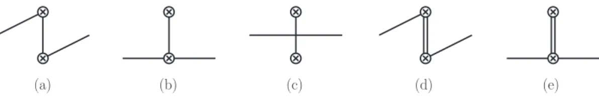
The different lattice contractions are pictorially represented in figure 2. We have two fully connected graphs C

and C

, a graph A in which the pion in annihilated by one current and created again by the second current, two graphs S

and S

with one disconnected quark loop, and a doubly disconnected graph D with two quark loops.

The symbols C

(y), C

(y), etc. denote contributions to the physical matrix ele- ments (2.1), i.e. it is understood that

• the contractions shown are averaged over the gauge ensemble and divided by the

ensemble average of the pion two-point function,

JHEP12(2018)061

• the two currents are inserted at the same time slice τ (i.e. y

= 0), and the ratio of four-point and two-point functions is evaluated at a plateau in τ . To use time reversal invariance, the plateau must be symmetric between source and sink times,

• both source and sink are projected on definite momentum p. By translation invariance one can thus shift their spatial positions by a common amount.

Details are given in section 3.3 below. For brevity, we do not indicate the dependence of C

(y) etc. on the pion momentum p.

From translation invariance one readily finds

M

(y) = M

( − y) for M = S

, D. (3.1)

Charge conjugation invariance gives

M

(y) = η

M

( − y) for M = C

. (3.2) If η

= − 1 one furthermore obtains M

(y) = 0 for M = A, S

, D. From P T invariance one gets

M

(y) = η

M

( − y) for M = C

, S

, S

, D, (3.3) M

(y) = η

M

(y) for M = A, C

, (3.4) where for the formulation of time reversal in the Euclidean path integral we refer to [14].

Finally, a useful relation for the contractions is obtained by taking the complex conju- gate of the contraction, followed by a parity transformation and charge conjugation. This gives

M

(y)

= η

M

( − y) for all contractions. (3.5) Combining (3.3) with (3.5) we find that C

, S

, S

and D are real valued, whereas combin- ing (3.4) with (3.5) gives

Re M

(y) = 1 2

M

(y) + M

( − y)

, i Im M

(y) = 1 2

M

(y) − M

( − y)

(3.6) for M = A, C

.

3.2 Physical matrix elements

The form of the relation between pion matrix elements and lattice contractions depends on the product of C parities. Using the shorthand notation

C

= C

(y) , C

= 1 2

C

(y) + C

( − y)

, A = 1 2

A

(y) + A

( − y) , S

= 1

2

S

(y) + S

( − y)

, S

= S

(y) , D = D

(y) , (3.7)

JHEP12(2018)061

Oi(y) Oi(y)

Oj(0) C₁^ij(y) =

= η^ij_C× C₂^ij(y) =

Oj(0)

Oi(y)

A^ij(y) =

Oi(y)

Oj(0) Oj(0)

S₁^ij(y) = = η^ij_C×

S₂^ij(y) =

Oi(y) D^ij(y) =

Oi(y)

Oj(0)

Oi(y) Oj(0)

Oj(0)

Oi(y) Oj(0)

Figure 2. Lattice contractions for the two-current correlation function (2.1) in a pion. The

dependence on the pion momentum p is not indicated for brevity. The product η

of charge

conjugation parities of the two operators is defined below (2.7).

JHEP12(2018)061

we have for η

= +1

h π

| O

(y) O

(0) | π

i = C

+

2S

+ D , h π

| O

(y) O

(0) | π

i =

2C

+ S

+

2S

+ D , h π

| O

(y) O

(0) | π

i =

2S

+ D

− A , h π

| O

(y) O

(0) | π

i = C

+

2S

+ D +

2C

+ S

+ A , h π

| O

(y) O

(0) | π

i = − C

+

2C

+ S

, h π

| O

(y) O

(0) | π

i = 2C

+ 2A ,

h π

| O

(y) O

(0) | π

i = 2C

(y) + S

+ A

(y) ,

√ 2 h π

| O

(y) O

(0) | π

i = C

+

C

(y) − C

( − y)

+ A

(y) . (3.8) One can verify that this satisfies the isospin relations in section 2.1. We have three inde- pendent real valued combinations, which can for instance be chosen as

1

2 F

(y) = h π

| O

(y) O

(0) | π

i + h π

| O

(y) O

(0) | π

i

= C

+ 2

2S

+ D

+ [2C

+ S

] , 1

2 F

(y) = h π

| O

(y) O

(0) | π

i − h π

| O

(y) O

(0) | π

i

= − C

+

2C

+ S

, 1

2 F

(y) = 1

2 h π

| O

(y) O

(0) | π

i

= C

+ A , (3.9)

where F

, F

and F

are the isospin amplitudes defined in (2.12). These combinations are real valued owing to (3.6), as the isospin amplitudes must be. The imaginary combination iF

of matrix elements can e.g. be isolated by

iF

(y) = h π

| O

(y) O

(0) | π

i − h π

| O

(y) O

(0) | π

i

= 2

C

(y) − C

( − y) +

A

(y) − A

( − y)

. (3.10)

In the present work, we only study the real valued combinations in (3.9).

For η

= − 1 we have three nonzero lattice contractions, C

, C

and S

, and two independent matrix elements, which may be taken as

h π

| O

(y) O

(0) | π

i = C

+ S

(y) − S

(y) ,

h π

| O

(y) O

(0) | π

i = 2C

+ S

(y) + S

(y) . (3.11) Among all contractions, C

has typically the smallest statistical uncertainties in the lattice simulation and thus plays a special role. The above equations show that it does not appear in isolation in any physical pion matrix element. However, C

can be regarded as

“approximately physical” in the following sense. Consider QCD with n

= 4 (instead of n

= 2) mass degenerate quarks, where SU(4) flavour symmetry is exact. It is easy to see that in this theory

h π

| O

(y) O

(0) | D

i = C

(y) , (3.12)

JHEP12(2018)061

ensemble β a [fm] κ L

× T m

[MeV] Lm

N

N

N

IV 5.29 0.071 0.13632 32

× 64 294.6(14) 3.42 2023 960 400 V 5.29 0.071 0.13632 40

× 64 288.8(11) 4.19 2025 984 400 Table 1. Details of the ensembles used in this analysis. N

is the total number of available gauge configurations and N

the number of configurations used in the present study. N

indicates the number of Wuppertal smearing iterations in the pion source. The error on the pion mass combines statistical and systematic errors, see [15]. The time difference between pion source and sink is t = 15a or t = 32a for both ensembles.

where the quark content of the D

meson is c¯ s. The correlation function C

computed in our study does not exactly correspond to this matrix element, because our lattice action has n

= 2 and not n

= 4 sea quark flavours. We therefore must interpret (3.12) within the partially quenched approximation.

3.3 Simulation details

Lattice action and quark mass values. We have performed N

= 2 lattice simulations with the Wilson gauge action and non-perturbatively improved Sheikholeslami-Wohlert (NPI Wilson-clover) fermions. The gauge configurations were generated by the RQCD and QCDSF collaborations. As is discussed for instance in [15, 16], there are eleven standard ensembles with pion masses down to 150 MeV. Two of these are used in the present study, namely ensembles IV and V, with a reduced number of gauge configurations as indicated in table 1.

We will also study the dependence of the pion matrix elements (2.1) on the quark mass. To this end, we have performed simulations with ensemble V and different values of κ in the quark propagator, namely

light quarks: κ = 0.13632 am

= 0.00291(3) , strange: κ = 0.135616 am

= 0.02195(3) ,

charm: κ = 0.125638 am

= 0.31475(3) , (3.13)

where we also give the values of the bare quark masses m

in lattice units. Here “light quarks” refers to the κ value of ensemble V, whereas the other two values correspond to the physical strange and charm quark masses, as determined in [17] and [18] by tuning the pseudoscalar ground state mass to 685.8 MeV in the first case and the spin-averaged S-wave charmonium mass to 3068.5 MeV in the second case. Since our simulations are performed with an n

= 2 fermion action, the strange and charm quarks are partially quenched.

Correlation functions. To compute the pion matrix element in (2.1) on a lattice in Euclidean space-time, we need the four-point correlators

C

(~y , τ, t) = a

X

~x ,~z

e

h 0 | Π(~x, t) O

(~y , τ) O

( ~ 0, τ ) Π

(~z , 0) | 0 i , (3.14)

JHEP12(2018)061

where Π(x) is a pion interpolator. We use interpolators with Dirac structure γ

. Pion matrix elements are extracted by calculating the following ratio at time slices where excited states should be suppressed:

h π(p) | O

(y) O

(0) | π(p) i = R

(~y ) = 2E

V C

(~y , τ, t) C

(t)

. (3.15)

Here V = L

a

is the spatial volume and C

(t) = a

X

~ x,~z

e

h 0 | Π(~x, t) Π

(~z , 0) | 0 i (3.16) the usual pion two-point function. In analogy to (3.14) and (3.15), we use an appropriate ratio of the three-point function C

(τ, t) and C

(t) to extract the matrix elements h π(p

) | O

(0) | π(p) i of the vector and scalar currents. We thus obtain the vector and scalar form factors for the pion, which are used in sections 3.4 and 5.3.

The pion energy in (3.15) is computed using the continuum dispersion relation E

= p ~p

+ m

, which is well satisfied for the momenta investigated here. The value of m

is obtained from an exponential fit of the two-point function, which gives

293 MeV (light, L = 40) , 299 MeV (light, L = 32) ,

691 MeV (strange, L = 40) , 3018 MeV (charm, L = 40) . (3.17) The statistical errors of the fits are less than 1%, and since we do not aim at a high-precision analysis, we do not attempt to quantify the uncertainty due to excited states. We observe that the values in (3.17) agree reasonably well with the pion masses given in table 1 for light quarks and quoted after (3.13) for strange quarks.

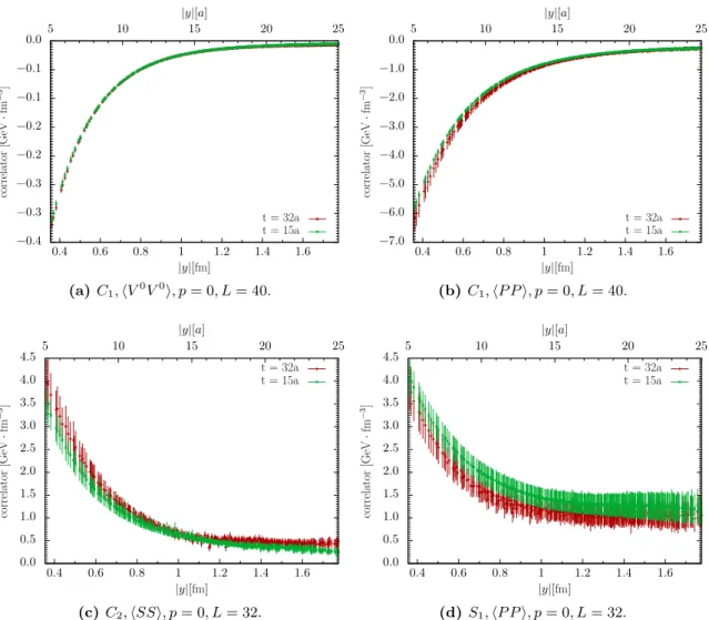
The source-sink distance is fixed to t = 15a ≈ 1.07 fm as a default. To investigate the influence of excited states, we have also calculated graphs C

, C

and S

with t/a = 32.

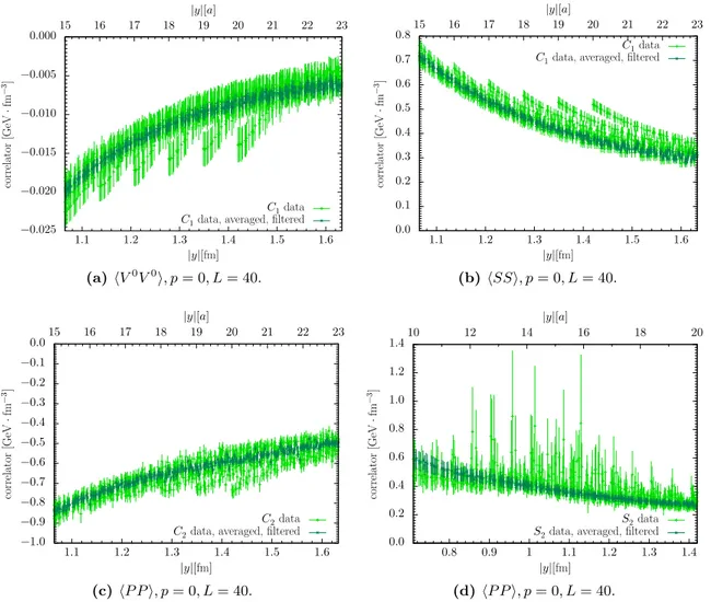
To extract the desired matrix elements, we calculate the ratio (3.15) by fitting or averaging over the plateau around τ = t/2. For the contractions C

and A, we measure the τ dependence of C

and fit to a plateau in the τ ranges specified in (4.1). For t/a = 15 we have S

data for τ /a = 7 and 8, which we average, whereas for the remaining contractions C

, S

and D we take τ /a = 7 or 8 for each gauge configuration on a statistical basis. We recall that the plateau extraction must be symmetric around τ = t/2 in order to respect the time reversal invariance relations of section 3.1. The data for C

and S

with t/a = 32 is restricted to τ /a = 16.

Details on the contractions. We now give details on the calculation of the different

lattice contractions for C

. Let us start with a broad overview, which is pictorially

represented in figure 3. Most graphs are calculated using the one-end trick [19] at the

source, which for A and C

we are also able to use at the sink. C

and S

have a similar

structure, for which the sequential source technique [20] is suitable. In general, loops are

obtained using stochastic insertions, except for the double-insertion loop of S

, where usual

point-to-all propagators are used. The D graph is calculated using point sources only. For

JHEP12(2018)061

0 τ t

~ y

× ×

× ×

Γ

Γ

C

× ×

× ×

Γ

Γ

A

B

B

×

×

Γ

×

Γ

C

×

×

Γ

×

Γ

S

G

L

×

×

Γ

Γ

S

G

L

Γ

× Γ

× D

G

L

L

point source/point-to-all-propagator stochastic source/propagator

×

seq. source (dashed)/seq. propagator hopping parameter expansion trick / current insertion/sink

Figure 3. Lattice methods employed for computing the different graphs of the four-point function.

Colours are used to distinguish the different parts of a graph. Two stochastic sources within a pion source or sink lead always to the application of the one-end trick or two-hand-trick, respectively.

the evaluation of the two-point graph G

and the connected part G

of the three-point graph (see figure 3) we alternatively use point sources or the one-end trick.

We use stochastic Z

⊗ iZ

wall sources, i.e. a set of complex random vectors η

carrying space-time, spin and colour indices (not explicitly written here). η

is nonzero only on the time slice t, where it has components ( ± 1 ± i)/ √

2 that are random for each gauge configuration. Averaged over all realisations, one then has

1 N

N_src^st

X

`

η

⊗ η

→ 1

, (3.18)

where the matrix 1

is unity if both time indices are equal to t and zero otherwise. Using this identity as an expression for the pion source represents the one-end trick.

The structure of graphs C

and A allows us to perform a second one-end trick at the

sink, which we refer to as the “two-hand trick”. For C

this trick was applied already

in [11]. In a different context it was used in [21], where it was dubbed the “stochastic

sandwich method”. Including the sign of the Wick contraction (easily obtained from the

JHEP12(2018)061

number of fermion loops) we explicitly have

C

(~y , τ, t) = a

V N

N_src^st

X

`

X

~x

h

Ψ

(~x + ~y , τ) γ

Γ

Ψ

(~x + ~y , τ) i

× h

Ψ

(~x, τ )γ

Γ

Ψ

(~x, τ ) i , A

(~y , τ, t) = − a

V X

~ x

D

B

(~x + ~y , τ )B

(~x, τ ) E + a

V X

~x

D B

(~x + ~y , τ) E D

B

(~x, τ ) E ,

B

(~x, τ) = 1 N

N_src^st

X

`

h

Ψ

(~x, τ )γ

Γ

Ψ

(~x, τ ) i

, (3.19)

where again V = L

a

is the spatial volume. Here and in the following, the notation h . . . i denotes the average over the gauge ensemble and [. . .] indicates a closed spin-colour structure. The vector Ψ

is obtained from an inversion of the Wilson-clover Dirac operator D on the random source,

D Ψ

= Φ E

η

, (3.20)

where

E

~x,~y

= e

δ

(3.21) is a diagonal matrix in the spatial coordinates. For better legibility, the (~x, t)-component of Ψ is written as Ψ(~x, t) rather than Ψ

in (3.19). We will use the same notation for other quantities that are vectors in space-time.

Source smearing is implemented by Φ, which is a hermitian matrix acting on spatial coordinates and colour indices and consists of 400 Wuppertal smearing iterations [22]. It turned out that taking Φ E

instead of E

Φ in (3.20) greatly improves the signal for nonzero momenta. This observation contributed to introducing momentum smearing in [23]. The contractions for which we have data with nonzero ~p are C

and A on the lattice with L = 40. Specifically, C

was computed for all 24 nonzero momenta satisfying p

≤ 3 and A for all 6 nonzero momenta with p

= 1. Here p is given as a multiple of the smallest non-trivial lattice momentum 2π/(La), which is equal to 437 MeV for L = 40.

As we see in (3.19), the calculation of A involves the subtraction of vacuum contri- butions in order to give the fully connected pion matrix element. For symmetry reasons, these subtractions are only nonzero for the currents A and P .

The connected part of graph S

is obtained by applying the sequential source method either to stochastic sources with the one-end trick (denoted by “oet”) or to point sources

2

Note that C

(~y , τ, t) is a contribution to the four-point correlator C

, whereas C

(y) introduced in

section 3.1 is a contribution to the pion matrix element (3.15). The same holds for the other contractions.

JHEP12(2018)061

(denoted by “pt”). The loop appearing in S

is calculated by using a stochastic source η

at time slice τ with the corresponding solution χ

of the Dirac equation,

D χ

= η

. (3.22)

Specifically, we have S

(~y , τ, t) = − a

V X

~ x

D

G

(~x + ~y , τ, t) L

(~x, τ ) E + a

V X

~x

D

G

(~x, τ, t) E DD

L

(τ ) EE ,

L

(~y , τ) = 1 N

N_ins^st

X

`

h η

(~y , τ)Γ

χ

(~y , τ) i

(3.23) and

DD

L

(τ ) EE

= a

V

X

~x

D

L

(~x, τ ) E

. (3.24)

Note that for symmetry reasons, the vacuum subtraction for S

in (3.23) is only nonzero for the scalar current S. If the one-end trick is used, then G

is given by

G

(~x, τ, t) = 1 N

N_src^st

X

`

h X

(~x, τ) γ

Γ

Ψ

(~x, τ) i

(3.25) with the sequential propagator X

(~x, τ) obtained by inversion of

D X

(~x

, t

) = δ

Φ E

Φγ

Ψ

(~x

, t

) . (3.26) We refrain from writing out the corresponding expressions for G

and X

with point sources, given that they are identical to those used in standard computations of the pion form factor, see e.g. [24]. We find very good agreement between S

computed with the one-end trick and with point sources, with slightly larger statistical errors for the latter. In later sections, only the one-end trick results are used. By contrast, we take the point-source version of G

to evaluate the connected contributions to the vector and scalar form factors.

The contraction C

has a similar structure as the connected part of S

, but it requires the calculation of an additional propagator between the two current insertions. For its evaluation we again use a stochastic source at the insertion time slice τ . To reduce statistical noise, we make the following improvements. We consider the hopping parameter expansion of the propagator [25–27], writing D = (1 − H)/(2κ) with the hopping term H, and make use of the geometric series:

M = D

= 2κ (1 − H)

= 2κ

∞

X

n=0

H

= 2κ

n(~y)−1

X

n=0

H

+ 2κ

∞

X

n=n(~y)

H

. (3.27) Since for the Wilson-clover action, H involves at most nearest neighbours on the lattice, one needs at least

n(~y ) =

3

X

i=1

min | y

|

a , L − | y

| a

(3.28)

JHEP12(2018)061

hopping terms to obtain a non-vanishing contribution to the propagator from a point ~x to

~x + ~y on a periodic lattice of spatial size La. Hence, the first sum on the r.h.s. of (3.27) can be omitted, and we get

M = 2κ

∞

X

n=n(~y)

H

= H

2κ

∞

X

n=0

H

= H

M for propagation from ~x to ~x + ~y , (3.29) where in the last step we used (3.27) again. Taking H

M instead of M itself, we implicitly omit those terms that do not contribute to the propagation but may add to the stochastic noise. The expression to be evaluated for the C

graph is then given by

C

(~y , τ, t) = a

V N

N_src^st

X

`

X

~x

h

X

(~x, τ )γ

Γ

ξ

(~x, τ ) i

× h

η

(~x + ~y , τ )Γ

Ψ

(~x + ~y , τ) i

(3.30) with

ξ

= H

χ

= H

D

η

. (3.31) For D and S

, one needs the pion two-point graph G

and two single insertion loops L

or one double insertion loop L

, respectively. For G

we again use either one-end trick or point sources. The double insertion loop is evaluated using a point source S

at x = ( ~ 0 , τ ), from which the point-to-all propagator M

is obtained by inverting

DM

= S

. (3.32)

Note that S

and hence also M

is a vector in space-time but a matrix in spin and colour.

The space-time components of the point source are S

(x

) = 1δ

. We then have L

(τ, ~y ) = tr n

γ

M

(~y , τ )γ

Γ

M

(~y , τ ) Γ

o

(3.33) with the trace referring to spin and colour indices, and

S

(~y , τ, t) = − D

G

(t) L

(~y , τ) E + D

G

(t) E D

L

(~y , τ ) E , D

(~y , τ, t) = a

V X

~ x

D

G

(t) L

(~x + ~y , τ ) L

(~x, τ ) E

− D

G

(t) E D

L

(~x + ~y , τ) L

(~x, τ ) E

− D

G

(t) L

(~x, τ ) E DD

L

(τ ) EE

− D

G

(t) L

(~x, τ ) E DD

L

(τ ) EE + 2 D

G

(t) E DD

L

(τ ) EE DD

L

(τ ) EE

(3.34) with hh L

ii defined in (3.24). When evaluated with the one-end trick, the two point graph reads

G

(t) = 1 N

N_src^st

X

`

Ψ

Φ E

ΦΨ

. (3.35)

JHEP12(2018)061

L = 40 L = 32

graph N

N

N

N

N

N

N

N

N

N

C

1 - - 1 L

1 - - 1 L

C

1 10 - 5 L

1 20 - 1 L

A 1 - - 4 L

1 - - 1 L

S

- - 120 4 L

- - 120 3 L

S

1 - - 16 16 1 - - 1 2

D - 60 60 1 L

- 60 60 1 L

Table 2. Numbers N

of stochastic noise vectors and numbers of sources and current insertions used for each graph in our simulations for the two lattice volumes. For most graphs, stochastic propagators are connected to the insertion, which implies an average over the entire spatial lattice volume. This is indicated by N

= L

.

Note that h L

i and h L

L

i depend on the distance ~y between the currents and can be nonzero for most combinations of Dirac matrices Γ

and Γ

. This makes vacuum subtrac- tions necessary for S

and D in most channels.

As indicated in (3.34), we use only stochastic sources for S

and only point sources for D. For the pion two-point function C

(t) = h G

(t) i , we compare both methods and find excellent agreement.

To increase statistics, we repeat the calculations at N

time positions t

of the source (keeping τ and t fixed relative to t

) and for several spatial insertion positions N

of the current. For most graphs, the latter is implicitly realised by using stochastic wall sources.

The corresponding numbers, as well as the size of the stochastic noise vector sets, are given in table 2. Note that in some cases these numbers differ between the lattices with L = 40 and L = 32 (ensembles V and IV of table 1).

3.4 Renormalisation

We convert all lattice currents, which are defined in the lattice scheme at a lattice spacing a, into the MS scheme at the renormalisation scale µ = 2 GeV. The corresponding renormal- isation constants depend on the gauge coupling g

= 6/β, where in our case β = 5.29. For currents with nonzero anomalous dimension, such as in the scalar and pseudoscalar cases, there is also a dependence on aµ. The conversion factors used for the correlator (3.15) of currents i and j read

R

= ˜ Z

Z ˜

R

with ˜ Z

= Z

(1 + am

b

) , (3.36)

see e.g. [15]. Here we have included the coefficients b

for the mass-dependent order a

improvement. They become particularly relevant at the charm quark mass. In the vector

and axial vector cases, there are additional mass-independent order a improvement terms

(accompanied by c

and c

, respectively), which we ignore in the present work. Note that

some of the matrix elements listed in section 3.2 receive contributions from flavour singlet

JHEP12(2018)061

S P V A T

Z

0.6153(25) 0.476(13) 0.7356(48) 0.76487(64) 0.8530(25)

b

1.3453 1.2747 1.2750 1.2731 1.2497

b

1.091(55) 1.586(32)

b

1.673 1.586 1.586 1.584 1.555

Table 3. Renormalisation factors Z

from [15] for the different currents (2.3) in the MS scheme at scale µ = 2 GeV. We also list the perturbative estimates of the coefficients b

from [15], the non-perturbative determinations (3.37) and (3.38), and the rescaled values (3.39). For the latter, we estimate an error of 34% as explained in the text.

current combinations. In these cases our renormalisation procedure should be regarded as approximate, because we do not take into account operator mixing.

The renormalisation factors Z

have been obtained in [28] (updated in [15]) in a two- step procedure: first the currents were matched non-perturbatively from the lattice scheme to the RI’/MOM scheme and then from there to the MS scheme in continuum perturbation theory. The coefficients b

= 1 + O (g

) have been computed in lattice perturbation the- ory [29–31]. Furthermore, in [32] the coefficient b

was determined non-perturbatively as

b

= 1 + 0.19246 g

1 − 0.3737g

1 − 0.5181g

(3.37)

with an uncertainty of about 5%. We can determine b

non-perturbatively by evaluating the vector form factor at zero momentum transfer with charm quarks (am

= 0.3147).

Multiplied by Z

(1 + am

b

) this must give 1, owing to charge conservation. Using the result F

(0) = 0.9068(2) from our L = 40 lattice and the value of Z

from [15], we extract

b

= 1.586(32) , (3.38)

where the uncertainty is dominated by the uncertainty on Z

.

Table 3 gives the values for Z

(2 GeV), as well as estimates b

using one-loop perturbation theory with an “improved” coupling constant (for details see (26) and (27) in [15]). In the next row, we give the non-perturbative estimates b

from (3.37) and (3.38).

We see that the non-perturbative value for b

is 24% larger than the perturbative estimate, while b

from [32] is about 19% smaller than the perturbative result. We remark that different non-perturbative determinations of b

only need to agree up to order a effects.

Based on our result for b

, we make the naive assumption that all non-perturbative coefficients are larger than the perturbative estimates and define rescaled coefficients

b

= b

b

b

, (3.39)

which are also listed in the table. As is clear from the scalar channel, there is a huge

uncertainty in this procedure. We find | 1 − b

/b

| = 34% and take this as our uncertainty

of the coefficients b

with i 6 = V . The results in the following sections are obtained with

the coefficients b

for i = S, V and with b

for all other currents.

JHEP12(2018)061

0 0.2 0.4 0.6 0.8 1 1.2 1.4

−15 −10 −5 0 5 10 15

𝑁(𝑡)𝐶4pt(𝑡,𝜏)/𝐶2pt(𝑡)[arbitr.units]

𝜏 − 𝑡/2 [𝑎]

𝐶₁,⟨𝐴⁰𝐴⁰⟩,𝑦 = (0, 3, 1)𝑎,⃗ 𝑝²= 0,𝐿 = 40

𝑡 = 32𝑎 𝑡 = 32𝑎(shifted𝜏 → 64 − 𝜏) 𝑡 = 15𝑎

(a) C

, hA

A

i, ~y /a = (0, 3, 1), p = 0, L = 40.

0 0.5 1 1.5 2 2.5 3 3.5 4 4.5 5

−4 −2 0 2 4

𝐶4pt(𝑡,𝜏)/𝐶2pt(𝑡)[arbitr.units]

𝜏 − 𝑡/2 [𝑎]

𝐴,⟨𝑆𝑆⟩,𝑡 = 15𝑎,𝑦 = (0, 3, 1)𝑎,⃗ 𝑝²= 0,𝐿 = 40

(b) A, hSSi, ~y /a = (0, 3, 1), p = 0, L = 40, t = 15a.

Figure 4. Dependence of the four-point function on the current insertion time τ at a fixed distance

~y between the two currents. Shown are the contributions of the contraction C

to the correlator h A

A

i and of the contraction A to h SS i . Here and in all following plots, errors are purely statistical.

The normalisation factor N (t) is specified in the text. p denotes the pion momentum and L the spatial lattice extent. Unless mentioned otherwise, all data shown in this paper are for light quarks.

4 Data quality and lattice artefacts

In this section we investigate the quality of our data and discuss a number of lattice artefacts. We concentrate on the data for light quarks here, for which we have the largest set of simulations. We verified that for heavy quarks, the lattice artefacts are not worse than for light ones.

4.1 Plateaux and excited state contributions

For the contractions C

and A, we have data for the ratio (3.15) of four-point and two-point functions in a wide range of the current insertion time τ and can hence verify the existence of a plateau. Figure 4 shows this ratio for two cases that are representative of channels with a good signal. In the case of figure 4(a) we have data for sink-source separations of t/a = 15 and 32, which we plot in such a way that the midpoints τ = t/2 coincide in both cases. Throughout this paper, error bars are purely statistical and determined by the jackknife method. To eliminate autocorrelations, we take the number of jackknife samples as 1/8 times the number N

of gauge configurations (see table 1).

The time separation t/a = 32 is half the temporal extent of our lattices, so that the pion two-point function C

(t) at that point has equal contributions from pions that propagate forward or backward from the source at time zero. To extract the pion matrix element, we must hence multiply C

(~y , τ, t)/C

(t) in (3.15) with a normalisation factor N (32a) = 2, which is also done in the figure. For t/a = 15, the contribution from backward propagating pions in the two-point function is below 3%. We do not correct for this contamination and take N (15a) = 1 in this case.

The data in figure 4 show a clear plateau around τ = t/2. In figure 4(a) the plateaux for

the two source-sink separations are in good agreement with each other, which indicates that

JHEP12(2018)061

contributions from excited states are not very large. Based on the plots and their analogues for other channels, we extract plateau values by fitting to a constant in the ranges

6 ≤ τ /a ≤ 9 for t/a = 15 ,

14 ≤ τ /a ≤ 18 and 46 ≤ τ /a ≤ 50 for t/a = 32 . (4.1) For t/a = 32 we thus combine the two plateaux around τ /a = 16 and 48.

Examples for the extracted two-current matrix elements as a function of the distance between the currents are shown in figure 5. Here and in the following, we write y = | ~y | . We see that the data for t/a = 15 and 32 are consistent within their statistical uncertainties.

In these plots and in their analogues for the other channels, we do not find any indication for large excited state contamination.

4.2 Anisotropy effects

In the continuum, the correlation functions h V

V

i , h A

A

i , h SS i and h P P i in a pion at rest can only depend on the modulus y = | ~y | . Lattice regularisation breaks rotational invariance, so that an anisotropy in the ~y dependence of our correlators is a clear indication of lattice artefacts.

At large distances y/a ∼ L/2 we see clear signs of anisotropy, as shown in figure 6(a) to (c). As explained in detail in [8], this can be traced back to the use of a finite lattice with periodic boundary conditions: the two currents are sensitive to the “images” of the pion in lattice cells adjacent to the elementary cell of size L

. At a given distance y, this effect is smallest for vectors ~y with directions close to space diagonals ( ± 1, ± 1, ± 1) and largest if ~y points along one of the coordinate axes. This gives rise to the distinct “sawtooth” pattern seen in our plots, which was also observed in earlier studies [8, 11]. An analytic investigation of the same phenomenon using a low-energy effective field theory can be found in [33]. A method to correct for these periodic images was proposed in [8] and employed in [11], where simulations were performed on L = 24 lattices with a ≈ 0.077 fm. The resulting physical length La was thus 0.81 times the length of the smallest lattice used in our study.

Benefiting from the larger size of our lattices, we take a less sophisticated approach here and consider only data for distances ~y close to the space diagonals. To this end, we use exact lattice symmetries to map the vector ~y into the octant where all its components are non-negative and define ϑ(~y ) as the angle between that vector and the diagonal (1, 1, 1).

We then retain only data points satisfying

cos ϑ(~y ) ≥ 0.9 . (4.2)

After this cut, we statistically average the correlators over points ~y of the same length y, which greatly decreases statistical errors. The points thus combined are not necessarily related by an exact lattice symmetry operation, and we checked that restricting the data combination to points that are equivalent on the lattice gives results consistent with those of the more inclusive combination.

As seen in figure 6(a) to (c), the above procedure efficiently removes anisotropy effects

while retaining enough data points. It also removes a broad anisotropic structure that we

observe for h P P i in the S

graph, figure 6(d), for which we have no interpretation.