supersymmetric Yang-Mills theory on the lattice

JHEP11(2018)092

Published for SISSA by Springer

Received : September 12, 2018 Accepted : October 30, 2018 Published: November 14, 2018

Adiabatic continuity and confinement in

supersymmetric Yang-Mills theory on the lattice

Georg Bergner, ^a Stefano Piemonte ^b and Mithat ¨ Unsal ^c

a Friedrich-Schiller-University Jena, Institute of Theoretical Physics, Max-Wien-Platz 1, D-07743 Jena, Germany

b University of Regensburg, Institute for Theoretical Physics, Universit¨ atsstr. 31, D-93040 Regensburg, Germany

c Department of Physics, North Carolina State University, Raleigh, NC 27695, U.S.A.

E-mail: georg.bergner@uni-jena.de, stefano.piemonte@ur.de, unsal.mithat@gmail.com

Abstract: This work is a step towards merging the ideas that arise from semi-classical methods in continuum QFT with analytic/numerical lattice field theory. In this context, we consider Yang-Mills theories coupled to fermions transforming in the adjoint representation of the gauge group. These theories have the remarkable property that confinement and discrete chiral symmetry breaking can persist at weak coupling on R ³ ×S ¹ up to small (non- thermal) compactification radii. This work presents a lattice investigation of a gauge theory coupled to a single adjoint Majorana fermion, the N = 1 Supersymmetric Yang-Mills theory (SYM), and opens the prospect to understand analytically a number of non-perturbative phenomena, such as confinement, mass gap, chiral and center symmetry realizations, both on the lattice and in the continuum. We study the compactification of N = 1 SYM on the lattice with periodic and thermal boundary conditions applied to the fermion field. We provide numerical evidences for the conjectured absence of phase transitions with periodic boundary conditions for sufficiently light lattice fermions (stability of center-symmetry), for the suppression of the chiral transition, and we provide also a diagnostic for Abelian vs.

non-Abelian confinement, based on per-site Polyakov loop eigenvalue distribution functions.

We identify the role of the lattice artefacts that become relevant in the very small radius regime, and we resolve some puzzles in the naive comparison between continuum and lattice.

Keywords: Confinement, Lattice Quantum Field Theory, Supersymmetric Gauge Theory, Wilson, ’t Hooft and Polyakov loops

ArXiv ePrint: 1806.10894

JHEP11(2018)092

Contents

1 Introduction 1

2 Adjoint QCD on the lattice 4

3 Order parameters for the phase diagram of adjoint QCD 6

4 The perturbative effective potential for the Polyakov loop on the lattice 7 4.1 Abelian vs. non-Abelian confinement regimes: first pass 12

4.2 Different Polyakov line effective actions 13

5 The phase diagram on the continuum and lattice 14 5.1 Explanation of the discrepancy of lattice and continuum 18 6 Numerical results for compactified adjoint QCD 20

6.1 Confined and deconfined phases in SYM theory 21

6.2 N _f = 2 QCD(adj) 23

6.3 Eigenvalue distributions and Abelian vs. non-abelian confinement 25

6.4 The Polyakov loop in the adjoint representation 28

6.5 The chiral condensate 29

7 Conclusions 30

1 Introduction

Confinement is a feature of strong interactions emerging in the long distance physics of certain non-Abelian gauge theories. The effective low energy degrees of freedom of these theories are colorless bound states which cannot be described as a simple combination of the elementary fields. The non-perturbative features of the strongly interacting regime, like confinement and the bound state spectrum, are consequently still beyond any analyti- cal understanding. Perturbation theory can provide a reliable approximation of scattering processes only at very high energy, but it cannot explain the structure and the properties of low energy states. Despite the success of the numerical lattice simulations in repro- ducing the observed hadron masses, an understanding of the nature of confinement is still missing on R ⁴ .

An interesting alternative analytical approach is based on a controlled semiclassical

analysis that tries to identify the most relevant field contributions as in the Polyakov

model on R ³ [1]. However, despite the important successes of the Polyakov model, the

idea remained dormant in QCD in four dimensions, mainly due to two reasons: one is that

it was often believed that the Polyakov mechanism was a manifestly three-dimensional

JHEP11(2018)092

mechanism, and the other is that in theories with exactly massless fermions, the Polyakov mechanism would not work [2]. About ten years ago, new ideas and techniques in semi- classics started to emerge and the utility of (justified) semi-classics into non-perturbative problems in QCD and other vector-like and chiral gauge theories has been realized [3–6].

For related earlier work, see [7–10].

More recently theories with matter fields transforming in the adjoint representation of the gauge group and certain supersymmetric theories became a valuable subject of these investigations [11, 12] using tools of resurgence, and Picard-Lefschetz theory. The QFT application of resurgence may potentially provide a rigorous non-perturbative definition of path integral in continuum QFT. At least, in certain quantum mechanical models with instantons, it is proven that path integral can be decoded into a full semi-classical resurgent expansion [13], and in certain asymptotically free two-dimensional QFTs, such as two- dimensional CP ^{N −1} and principal chiral models, ideas related to resurgence have been fruitful to partially resolve the renormalon problem [14–16].

The semiclassical analysis corresponds to a sum of the expansions around the dominant field configurations in a regime where weak coupling methods are reliable. (See [14] for a recent review.) The inclusion of non-trivial configurations should overcome the limitation of standard perturbation theory by incorporating exponentially small non-perturbative effects of the form e ^−A/(g

^{N )} where A is pure number and (g ² N ) is the ’t Hooft coupling. ¹ If the time dimension is compactified and the length of the compact dimension R is smaller than the strong scale Λ ⁻¹ , the theory becomes weakly coupled due to asymptotic freedom. In this regime, QCD and Yang-Mills theories are in the deconfined phase as can be shown by studying the Gross-Pisarski-Yaffe (GPY) potential [17]. Consequently this region is disconnected by a phase transition (or crossover) from the large R low energy confined phase that one aims to understand. Furthermore, the dynamics of the theory at distances much larger than R is governed by a 3d pure Yang-Mills theory, which develops the strong (magnetic) scale on its own.

The situation is different in a gauge theory where the fermion fields are in the adjoint representation and fulfill periodic boundary conditions in the compact direction. Periodic boundary condition in path integral formalism map to

Z(R, m) = tr ˜ ^h e ^{−R H(m) ˆ} (−1) ^{F i} (1.1) in the operator formalism, where ˆ H(m) is the Hamiltonian operator and m is the fermion mass. This trace is a graded state sum which assigns an over-all (+1) sign to boson states and (-1) to fermion states. Note that (1.1) for N f = 1 and m = 0 is the well-known Witten index [18]. For general N _f or m 6= 0, the trace is a (non-thermal) twisted partition function which probes the phase structure of the theory as a function of R [4, 19].

If we consider the one-loop GPY potential with this partition function, the center- destabilizing potential induced by gauge bosons is overwhelmed by the center stabilizing contributions from sufficiently light fermion fields [20, 21]. In this case, the small R regime

1

Note that this type of non-perturbative effect is exponentially larger than the usual four-dimensional

instanton effects in gauge theories, which are of the form e

.

JHEP11(2018)092

is in a center symmetric phase on R ³ × S ¹ which is non-perturbatively calculable by semi- classical methods. The theory exhibits the semiclassical magnetic bion mechanism of con- finement, a non-perturbative mass gap for gauge fluctuations, and, if it exists in the theory, a discrete chiral symmetry breaking.

The small R regime on R ³ × S ¹ provides a controlled semi-classical approximation in sharp distinction from the so-called dilute instanton gas picture on R ⁴ which is an uncontrolled approximation, see section “the uses of instantons” in [22] and [23] for the limitations of the latter approach. The calculable semi-classical regime might in certain cases be smoothly connected to the confined strongly coupled regime at large R [4–6, 24].

This is the notion of adiabatic continuity which posits that a semi-classical calculable regime, under appropriate conditions, may be smoothly connected to a strong coupling regime without any intermediate phase transitions.

An exact cancellation between fermion and boson perturbative contributions occurs in the particular case of the N = 1 Supersymmetric Yang-Mills theory (SYM) or N _f = 1 QCD(adj) [10, 25]. Both center-stability as well as confinement of compactified SYM are solely due to non-trivial semiclassical contributions, namely neutral and magnetic bions.

The phase structure of gauge theories with N _f adjoint Majorana fermions, N _f -flavour QCD(adj), opens therefore a promising perspective for the understanding of the mecha- nisms of confinement [4, 11], see also [26–28].

A regularization providing a-priori non-perturbative numerical simulations is required to prove this continuous connection of the small R regime to the strongly coupled large R confined phase and to verify the absence of intermediate phase transitions. Monte-Carlo lattice simulations are an ideal first principles method from this point of view.

The first observation of the absence of deconfinement in compactified supersymmetric Yang-Mills theory has been presented in an earlier publication [29], we are investigating the phases of the theory more closely in this work. In order to understand the influence of the lattice discretization, we first compare the perturbative analysis in the continuum and on the lattice. It turns out that the discretization of the fermion action on the lattice is of particular importance in the small R regime. Due to lattice artefacts, the exact cancella- tion between fermion and boson contributions can only be achieved in the continuum limit.

Nevertheless we show that qualitative features of the semiclassical predictions are repro- duced on the lattice. In contrast to our earlier investigations we concentrate here on a fixed scale approach which avoids additional complications introduced by a variation of the lat- tice spacing. Part of the work is done with a clover improved Wilson fermion action in order to reduce the discretization effects. We consider the order parameters for the chiral and the deconfinement transition. The primary focus is on supersymmetric Yang-Mills theory, but we have also investigated the N _f dependence in a numerical study of N _f = 2 QCD(adj).

We introduce the lattice formulation and the order parameters for the investigations

of the phase transitions in the next two sections. In section 4 we provide a detailed

discussion of the perturbative effective potential of the Polyakov loop on the lattice and

in the continuum. Based on the analysis of the effective potential, we derive predictions

of the phase diagram of QCD(adj) in the weak coupling regime and conjectures about the

general phase diagram in section 5. After these theoretical considerations, we present our

JHEP11(2018)092

numerical results in section 6. The signals for deconfinement are investigated in N _f = 1 and N f = 2 QCD(adj). In addition we present results for the per-site constraint effective potential of the Polyakov line phase, the adjoint Polyakov loop, and the chiral condensate in the N _f = 1 case.

2 Adjoint QCD on the lattice

QCD(adj) consists of a non-Abelian gauge-field A ^c _µ (x) minimally coupled to N f Majorana fermions λ ^c _i (x). The expression of the continuum action is similar to QCD

S = Z

d ⁴ x







− 1

4 F µν F ^µν + 1 2

N

X

i=1

λ ¯ i D / + m λ i







= S g + S f , (2.1)

where F µν is the field strength tensor and the covariant derivative D µ acts in the adjoint representation. ² We consider SU(N _c ) gauge groups and we focus our numerical simulations only on N c = 2. Two Majorana spinors can be combined to a single Dirac spinor. Hence the counting of Majorana flavors N _f corresponds formally up to a factor 1/2 to the Dirac flavour counting used in QCD. The special case of N _f = 1 QCD(adj) is N = 1 super- symmetric Yang-Mills theory (SYM) and the fermion λ is called gluino, the superpartner of the gluon. Supersymmetry is obtained in the massless limit since a finite m breaks supersymmetry softly.

The lattice discretization of QCD(adj) can be chosen in several different ways. We use for the discretization of S g the tree level Symanzik improved gauge action, composed of square and rectangular Wilson loops of size 1 × 2 (W µν ^(2,1) ) and 1 × 1 (W µν ^(1,1) ),

S g = − β N _c



 5 3

X

x,µ>ν

Tr ⁿ W _µν ^(1,1) (x) ^o − 1 12

X

x,µ>ν

Tr ⁿ W _µν ^(2,1) (x) + W _νµ ^(1,2) (x) ^o



 . (2.2) The discretization of S f is more involved. According to the Nielsen-Ninomiya theo- rem the implementation of a local Dirac operator on the lattice either leads to additional fermion degrees of freedom (doublers) or requires the breaking of chiral symmetry. In our approach we use a Wilson-Dirac operator which introduces an additional spin-diagonal term to decouple the doubler modes at the cost of an explicit chiral symmetry breaking, see e.g. for a description of doublers and Wilson term [30]. ³ The fermion part of our lattice action is

S _f = 1 2

X

xy

λ ¯ _x (D _w ) _xy λ _y , (2.3)

2

A summation of colour indices is assumed.

3

Overlap and domain wall fermions would be an alternative with a more controlled chiral symmetry

breaking but their computational cost is quite demanding. Staggered fermions have been used in earlier in-

vestigations of QCD(adj), but they introduce additional degrees of freedom (tastes) and represent effectively

theories with larger N

if rooting is not included.

JHEP11(2018)092

with the Wilson-Dirac operator

(D w ) x,a,α;y,b,β = δ xy δ a,b δ α,β − κ

4

X

µ=1

(1 − γ µ ) _α,β (V µ (x)) ab δ x+µ,y

+(1 + γ _µ ) _α,β V _µ ^† (x − µ)

ab δ x−µ,y

− κc _sw

2 δ _xy σ _µν F ^µν , (2.4) where V µ (x) are the link variables in the adjoint representation and F µν is the clover pla- quette. The hopping parameter κ is related to the bare gluino mass m ₀ via κ = 1/(2m ₀ +8).

We have explored different strategies for the tuning of the gauge coupling β = ^2N _g

and of the parameters of the Wilson-Dirac operator. The first natural choice is the same setting as employed in earlier investigations of the bound states of the theory [31]. In these simulations the clover coefficient c sw has been set to zero and one level of stout smearing has been applied on the links V _µ (x) of the Dirac operator. In this framework β = 1.75 is good compromise between the simulation cost and the control of lattice supersymmetry breaking [31, 32]. In an alternative setup, we have also simulated the theory using un- smeared links and c _sw = 1, such that the leading order chiral symmetry breaking effects are removed from on-shell quantities [33]. Different lattice actions provide the same infor- mation about the phase structure of the theory up to lattice discretization errors, enabling us to check the reliability and the consistency of our simulations.

The integration of each Majorana fermion field yields the Pfaffian Pf(CD w ), where C is the charge conjugation matrix. The Pfaffian is real but not necessarily positive on lattice.

In the continuum limit, the Pfaffian is real and positive. A sign problem appears in the Wilson formulation for odd N _f in regions where the mass of the “adjoint pion”, the lightest gluino-ball, is small and lattice artefacts are dominant. The sign problem vanishes in the continuum limit. Based on our previous experience of lattice simulations of N = 1 SYM, we already know in the bare parameter space where the contribution from negative Pfaffian configurations is negligible. A positive Pfaffian is assumed in the following sections.

In numerical simulations the lattice extend is finite in all directions. Periodic boundary conditions are always applied in the three spacial directions. Our aim is the investigation of the compactified theory on a torus. Hence the extend in the spacial directions is assumed to be large enough to emulate the infinite volume limit and the temporal direction is compactfied:

T ³

|{z}

large

×S ¹ ≈ R ³ × S ¹ (2.5)

If fermions fields fulfill anti-periodic boundary conditions in the S ¹ direction, the theory on the T ³ × S ¹ torus emulates the thermal partition function of a quantum field theory in a box. If periodic boundary conditions are applied to fermion fields on S ¹ direction, the theory on T ³ × S ¹ corresponds to the twisted partition function (1.1) with no thermal interpretation. The latter setup is useful to realize the notion of adiabatic continuity.

Lattice simulations have to challenge discretization and finite volume effects. Finally,

numerical instabilities of the Rational Hybrid Monte Carlo algorithm forbid simulations

at very small gluino masses. Hence SYM can be simulated only with a non-vanishing soft

JHEP11(2018)092

supersymmetry breaking mass term. The continuum limit and the massless limit must be extrapolated from the numerical data.

3 Order parameters for the phase diagram of adjoint QCD

The lattice action is invariant under center symmetry transformations, corresponding to the multiplication of the gauge links in time direction on a given time-slice with a discrete phase rotation exp (iφ n ) with φ n = 2πn/N c . The deconfinement transition is identified with the spontaneous breaking of this symmetry at high temperatures. The quark fields in QCD, which are fermions in the fundamental representation, break center symmetry explicitly if one imposes periodic or anti-periodic boundary conditions. This symmetry is, however, preserved for fermions in the adjoint representation.

The Polyakov loop is the order parameter of the deconfinement phase transition. It is the path ordered product of the links in the fundamental representation along a line which wraps in the compact direction

P L = 1 N c V 3

X

~ x

TrW ^(N

⁾ (~ x) = 1 N c V 3

X

~ x

Tr ( _N

Y

t=1

U 4 (~ x, t) )

, (3.1)

where V ₃ denotes the three-dimensional lattice volume of the non-compactified directions.

The confined and deconfined phases are distinguished by a zero or non-zero expectation value of P _L . We consider in addition the Polyakov loop in adjoint representation P _L ^A , the path ordered product of links in the adjoint representation. The adjoint Polyakov loop is not an order parameter of the deconfinement transition due to the screening of the adjoint color charge. More generally arbitrary windings n of the Polyakov loop can be considered

P _L ⁽ⁿ⁾ = 1 N _c V ₃

X

~ x

Tr ^h W ^(N

⁾ (~ x) ^{n i} , (3.2) which is equivalent to consider loops in all representations. The eigenvalues of the Polyakov line W ^(N

⁾ play an important role in the discussions of the perturbative effective action in section 4.

In the massless limit, classical SYM has an additional U(1) chiral symmetry λ → exp {−iθγ ₅ }λ. This is not a symmetry in quantum theory due to the global Adler-Bell- Jackiw anomaly. The genuine symmetry of the quantum theory is Z 2N

in case of the gauge group SU(N c ). The discrete symmetry is broken spontaneously to Z 2 , and the theory has N _c isolated discrete vacua. The chiral condensate is the order parameter for this transition.

It is defined as the derivative of the logarithm of the partition function with respect to the fermion mass, equal to the expectation value of the quark bilinear h λλi. This operator is ¯ multiplicatively and additively renormalized in the Wilson formulation of lattice fermions.

In case of N f > 1 more general condensates like hdet(λ _i λ j )i are possible [4] which we have not considered in our present work.

A susceptibility can be defined for the order parameters O as

χ _O = V hO ² i − hOi ² , (3.3)

JHEP11(2018)092

where V is the three-dimensional volume for the Polyakov loop or the four-dimensional volume for the chiral condensate. The phase transition can be identified by the peak of the susceptibility and the divergence of this peak in the infinite volume limit. The susceptibility is subject to rather large finite volume corrections. The Binder cumulant,

B ₄ (O) = 1 − 1 3

hO ⁴ i

hO ² i ² , (3.4)

provides a signal with smaller finite size corrections. The deconfinement transition is expected to be in the three-dimensional Ising universality class [34], and the B 4 value at the transition should be 0.46548(5) [35], while in the confined and deconfined phase it is equal to zero and 2/3 respectively.

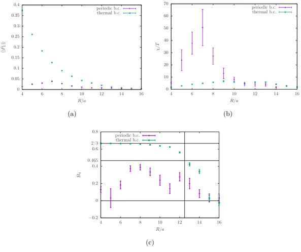
In previous numerical simulations we have determined the deconfinement and chiral transitions in SYM at finite temperature. With thermal boundary conditions, the temper- ature corresponds the inverse of the compactification radius T = 1/R. We have been able to observe a significantly different behaviour in the case of periodic boundary conditions for fermion fields in [29], by exploring the phase diagram in the space of the bare lattice parameters β and κ at fixed N t . The deconfinement transition line does not intersect the critical line corresponding to the zero renormalized gluino mass. The clear separation of the two lines is already a signal of continuity, but the control of lattice artefacts and the interpretation of the phase diagram in terms of renormalized physical quantities is diffi- cult. We follow a different approach in the present work. We keep fixed bare parameters, therefore the lattice spacing a and the gluino mass are constant, and the length of the compactification radius is changed by changing the number of lattice points N t = R/a in the temporal (compactified) direction.

4 The perturbative effective potential for the Polyakov loop on the lattice

The confined and deconfined phases as a function of R, m and N _f can be inferred from the effective potential of the Polyakov line that can be calculated straightforwardly in the one-loop approximation. The effective potential is usually identified with the free energy density at a constant background gauge field G _µ , which is at one loop level determined from the quadratic fluctuations. The background is chosen such that the link in time direction G ₄ is diagonal and all other links are set to the identity. In the case of SU(2) we have

G ₄ = e ^iφ/N

0 0 e ^−iφ/N

!

, (4.1)

and Polyakov loop then reads P _L = 1

2 Tr ( _N

Y

t=1

G ₄ )

= 1

2 Tr e ^iφ 0 0 e ^−iφ

!

= cos(φ) . (4.2)

Confinement (center-stability) is realized if the minima of the effective potential for the

Polyakov line phase (holonomy) φ is located at φ = π/2 mod π. In the deconfined phase

JHEP11(2018)092

there is a minimum at φ = 0 mod π. For a general SU(N _c ) gauge group, the background configuration is

G ₄ = diag ^h e ^iφ

^/N

, e ^iφ

^/N

, . . . , e ^iφ

^/N

ⁱ , (4.3) where φ N

= − ^{P N} _i=1

⁻¹ φ i and

P _L = 1 N c

Tr ( _N

Y

t=1

G ₄ )

= 1 N c

Tr











 e ^iφ

e ^iφ

. ..

e ^iφ













(4.4)

The effective potential of QCD(adj) in the one loop approximation is the sum of gluons, ghost, and fermion contributions. On the lattice the gauge links with the fluctuating field A _µ around the constant background G _µ are represented as

U _µ (x) = G _µ exp{igA _µ (x)} , (4.5)

and the gluon action is expanded in a power series of g. The kinetic part of the gluon Lagrangian is

L _gl = 1

2 Tr ⁿ D _µ ⁺ A _ν (x)D ⁺ _µ A _ν (x) ^o (4.6) where the gauge fixing term

S _gf = ^X

x,µν

Tr ⁿ D ⁻ _µ A _µ (x)D _ν ⁻ A _ν (x) ^o (4.7) has been added to the action to fix the gauge of the field A µ (x) while preserving gauge invariance with respect to background field G _µ . Only the standard Wilson plaquette action part is relevant in this computation. D ⁺ and D ⁻ denote the forward and backward lattice covariant derivatives

D _µ ⁺ = 1 a

G ^† _µ (x)A _µ (x + µ)G _µ (x) − A _µ (x) (4.8) D _µ ⁻ = 1

a

A µ (x) − G ^† _µ (x − µ)A µ (x − µ)G µ (x − µ) . (4.9) The kinetic part of the ghost field η is similarly

L _gh = 1

2 Tr ⁿ D _µ ⁺ η(x)D ⁺ _µ η(x) ^o ; (4.10) the last contribution comes from the Wilson fermion action (m ₀ = am)

L _f = 1 2

N

X

f=1

λ ¯ ^f (x) (

γ _µ D _µ ⁺ + D ⁻ _µ

2 + arD ⁺ _µ D _µ ⁻ + m )

λ ^f (x) . (4.11) The action is quadratic in fluctuating fields A µ , η and λ in the one-loop approximation, therefore these fields can be integrated out leading to

V ₃ V _eff = 4

2 − 1

log det D _µ ⁻ D ⁺ _µ − N _f

2 log det γ _µ D ⁺ _µ + D _µ ⁻

2 + arD _µ ⁺ D ⁻ _µ + m

!

= log det D _µ ⁻ D _µ ⁺ − N _f log det 1

4

D _µ ⁺ + D ⁻ _µ ² + arD _µ ⁺ D ⁻ _µ + m ²

. (4.12)

JHEP11(2018)092

Each boson field contributes to V _eff with a prefactor + ¹ ₂ , and each fermion field with a prefactor −1. The first term comes from the gauge part of the action, with a prefactor which counts four boson fields A _µ minus the fermion ghost field η. The last term is the contribution from the Majorana fermions with an additional factor ¹ ₂ due to the fact that integrating our fermion induce a Pfaffian.

The effective potential (4.12) shows clearly how a mismatch between fermion and boson contributions is introduced by the lattice discretization. The Wilson fermions have a different derivative operator and an additional momentum dependent mass term in order to remove the doubling modes. In the continuum, a more compact expression for V eff is obtained in the massless case. It can be recovered in the naive a → 0 limit of (4.12)

V 3 V eff = (1 − N f ) log det D ² , (4.13) since log det( D) = / ¹ ₂ log det( D / / D) = ¹ ₂ log det(D ² ). In this limit the difference between the boson and fermion derivative operators disappears. Gluon and adjoint fermion fields have an opposite contribution to the one-loop effective potential of the Polyakov loop which can- cel exactly in the continuum if N _f = 1, i. e. in the case of the N = 1 SYM. Supersymmetry ensures that this result holds to all orders of perturbation theory. In continuum N = 1 SYM theory, center stability is driven by pure non-perturbative effects [19]. For N _f > 1 continuum QCD(adj), the center-stability is a one-loop perturbative effect. However, the supersymmetry between gluons and gluinos of SYM is violated on the lattice, and V eff dif- fers from zero for non-zero lattice spacings. This mismatch will play an interesting role in section 5.1 in order to explain the difference of the lattice and continuum phase diagram.

The effective potential for the Polyakov line holonomies φ _a (or their differences φ _ab = φ _a − φ _b ) can be further simplified in momentum space [36, 37]. Assuming an infinite spacial extend of the lattice, an ∞ ³ × N t site lattice, and neglecting holonomy independent contributions, we obtain the following representation

V _eff ({φ _a }) = ^X

a6=b

V _eff (φ _ab ) =

N

−1

X

k=0

X

a6=b

Z π

−π

dp 2π

3

( log

p ˆ ² + 4 sin ²

φ _ab + 2πk 2N t

− N _f log

"

ˆ ˆ

p ² + sin ²

φ _ab + 2πk N t

+

m ₀ + r 2

p ˆ ² + 4 sin ²

φ _ab + 2πk 2N t

2 #)

, (4.14)

where the lattice momenta ˆ p and ˆ p ˆ are defined as p ˆ ² =

3

X

i=1

4 sin ² p i

2

and p ˆ ˆ ² =

3

X

i=1

sin ² p i . (4.15)

Consider first r = 0 and m 0 = 0, and set the holonomy field to zero in (4.14). The

difference between boson and fermion derivatives on the lattice is essentially reflected in ˆ p ²

vs. ˆ p ˆ ² . In fact, for bosons, the inverse propagator vanishes only at the origin of the Brillouin

JHEP11(2018)092

zone, as in the continuum case. However, for fermions, the inverse propagator is zero at all sixteen corners of Brillouin zone, (0, 0, 0, 0), (±π, 0, 0, 0), . . . , (±π, ±π, ±π, ±π). The corners except the origin are referred to as doublers, and undesired from the continuum point of view. On the lattice, the Wilson term proportional to r leads to a momentum dependent mass that removes the doublers in the continuum limit. The Wilson term lifts the doublers by making the modes at p _µ ∼ π acquire a mass of the order of cut-off, i.e.

proportional to the inverse lattice spacing. However, the Wilson term explicitly breaks chiral symmetry, as a consequence the fermion mass is both additively and multiplicatively renormalized.

The difference of the fermion determinants of the free theory is a shift of the modes in the compact or temporal direction by φ _ab . This result generalizes to any kind of fermion operator that can be implemented on the lattice: the effective potential is easily derived from a shifted momentum space representation. The shifts for the adjoint representation are ^φ _N

t

, for the fundamental one they would be _N ^φ

t

. In the case of SU(2) there is only one shift for the adjoint representation: φ ₁₂ = −φ ₂₁ = 2φ.

The effective potential for φ ab can be translated into an effective potential of different windings of the Polyakov loop. Again up to constant expressions, the quadratic potential

V _eff ({φ _a }) =

∞

X

n=1

X

a6=b

V _eff ⁽ⁿ⁾ e ^irφ

= N _c ²

∞

X

n=1

V _eff ⁽ⁿ⁾ P _L ^{(n) 2} + const (4.16)

is obtained. The coefficients V _eff ⁽ⁿ⁾ are the Fourier transform of V eff (φ ab ) with respect to φ ab

V _eff ⁽ⁿ⁾ = Z 2π

0

dφ _ab

2π e ^−irφ

V eff (φ ab ) . (4.17) After some algebra, the following expression is obtained for the coefficients V _eff ⁽ⁿ⁾

V _eff ⁽ⁿ⁾ = N _t Z π

−π

dω 2π e ^irN

^ω

Z π

−π

dp 2π

3

log







p ˆ ² + 4 sin ^{2 ω} ₂

h p ˆ ˆ ² + sin ² (ω) + m ₀ + ^r ₂ p ˆ ² + 4 sin ^{2 ω} ₂ ^{2 i N}





 . (4.18)

If the coefficients V _eff ⁽ⁿ⁾ are positive for n ≤ b ^N ₂

c, Z N

center-symmetry is preserved and the minimum of the potential is at P _L ⁽ⁿ⁾ = 0 for n 6= 0 mod N _c ; i.e, the expectation value of the Polyakov loops with winding number n 6= 0 mod N c is zero.

If some of the V _eff ⁽ⁿ⁾ are negative for n ≤ b ^N ₂

c, a corresponding subset of Polyakov loops will develop non-zero expectation values. In fact, if V _eff ⁽ⁿ⁾ < 0 for n = 1, then so are all higher n. In this case, Z N

center-symmetry is completely broken. If V _eff ⁽ⁿ⁾ < 0 for 1 ≤ n ≤ k ≤ b ^N ₂

c, then the center symmetry may break to different discrete subgroups that can be easily determined.

Note that an increase of ¹

V

indicates also an increasing susceptibility of the Polyakov

line with winding number n, providing a signal for the effective potential investigated in

section 6.

JHEP11(2018)092

− 0.03

−0.025

− 0.02

− 0.015

− 0.01

− 0.005 0 0.005 0.01 0.015 0.02

0 1 2 3 4 5 6

V

φ

N

= 0, N

= 4 N

= 0, N

= 6 N

= 0, N

= 8 N

= 1, N

= 4 N

= 1, N

= 6 N

= 1, N

= 8

Figure 1. One-loop effective potential for the Polyakov loop phase φ in SU(2) SYM on the lattice for different N _t at m ₀ = 0 comparing pure gauge (N _f = 0) and SYM (N _f = 1). The SYM effective potential is different from zero due to lattice artefacts. It is confining and the expected flat behavior is reached only asymptotically at large N t . The potentials are normalized to zero at φ = 0 in this plot.

We have computed the one-loop effective potential of SU(2) SYM on the lattice (4.12) or equivalently (4.14) for several values of N t . Clearly, unlike the continuum supersymmet- ric theory, for which the effective potential is zero to all orders in the perturbative expansion due to supersymmetry, the one-loop potential in the lattice formulation (4.12), (4.14) is actually non-vanishing,

V eff, continuum ({φ _a }) = 0, V eff, lattice ({φ _a }) = N _c ²

∞

X

n=1

V _eff ⁽ⁿ⁾ P _L ^{(n) 2} with V _eff ⁽ⁿ⁾ > 0 for n ≤ N c

2

. (4.19) This is hardly surprising because the lattice formulation based on Wilson fermions does not respect supersymmetry, and as such, we indeed expect a potential to be induced at one-loop order. The correct continuum limit is approached as R/a goes to infinity, which means the lattice spacing goes to zero at fixed physical R.

Remarkably, Wilson fermions with Wilson parameter r = 1, even when the effect of doublers is maximally lifted, have a stronger confining effect than continuum fermions, see figure 1, and lead to center stability even at one-loop level. In this respect, lattice SYM is similar to the N _f > 1 continuum QCD(adj) [38]. The one-loop prediction is a center-symmetric (confined) phase in the small R regime at a given fixed lattice spacing and m 0 = 0. In the small R/a regime, the dynamics probes higher scales towards the cutoff 1/a. At these scales the doubling modes that are lifted with masses of the order of the cutoff are still relevant and have a confining effect.

If the mass is increased, a phase transition to a deconfined phase occurs [38], calculable both in lattice perturbation theory and by continuum methods, as discussed in section 5.

This phase is connected to the deconfined phase of pure Yang-Mills theory. At N _c > 2

JHEP11(2018)092

the deconfinement transition is replaced by a transition to several intermediate phases with partially broken gauge symmetry, corresponding to the Higgs phases in the Hosotani mechanism [39]. The deconfined phase connected to the pure Yang-Mills case is reached increasing R after crossing these additional phases.

4.1 Abelian vs. non-Abelian confinement regimes: first pass

In the following we discuss in more detail the particular features of the confinement mech- anisms at small radius that arise in QCD(adj) at non-zero lattice spacing in the N _f = 1 case and also for N _f > 1.

The unbroken center symmetry at any R ∈ [0, ∞) does not have a unique implication for the Polyakov loop eigenvalues. Originally, Polyakov thought that the phases of the loop would have completely random fluctuations as origin of the a vanishing expectation value for the Polyakov line operator in the confined phase. However, from the analysis of the confining perturbative effective potential we obtain two different pictures. Indeed, both at small and large-R, hP _L i = 0, but at small-R the (untraced) Polyakov line is essen- tially e ⁱ

0

0 e ⁻ⁱ

!

with small-fluctuations around it. We refer to this regime as Abelian confinement regime, where the theory dynamically abelianized due to the induced poten- tial (4.12), (4.14). ⁴

At large-R, the theory is strongly coupled at the compactification scale and the fluctu- ations of the Polyakov loop eigenvalues are random as it can be seen from simulation results presented in section 6.3. We refer to this regime as non-Abelian confinement regime.

Some intuition for the large-R case may be gained from strong coupling lattice per- turbation theory. However, note that the strong coupling here refers to the bare lattice coupling at the cut-off. The strong coupling regime of lattice theory is not necessarily con- tinuously connected to the continuum physics, yet the strong coupling expansion provide some insights to understand lattice results. In particular, at infinite bare coupling, β = 0, we can ignore the action and the first term in the strong coupling expansion is the reduced Haar measure with an effective potential for the Polyakov line eigenvalues

V _Haar = − 1 2

X

a6=b

log

sin ² φ _ab

2

. (4.20)

The reduced Haar measure will always drive the theory to the confined phase. Since we are discussing the continuum physics that arises from bare weak coupling (as per asymptotic freedom) of lattice field theory, we will not discuss strong coupling expansion. Nevertheless

4

Dynamical abelianization is interesting on its own right, and the class of theories we are examin- ing exhibits some differences from other calculable confining QFTs. In Georgi-Glashow model in three- dimensions [1, 40, 41] and Seiberg-Witten theory in four-dimensions [42], the long distance theory abelian- izes due to a tree-level (classical) potential. In QCD(adj), at tree level, there is no potential for Polyakov loop. It is dynamically induced at one loop level, and leads to abelianization of the long distance theory [4].

Dynamical abelianization should also not be confused with ’t Hooft’s maximal abelian gauge proposal [43],

which enforces abelianization by hand as a gauge choice. Needless to say, this is done in the QFT which

becomes strongly coupled at large-distance and in particular, is not semi-classically calculable.

JHEP11(2018)092

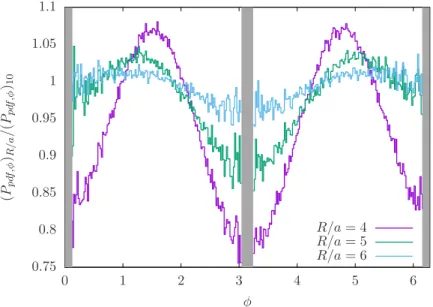
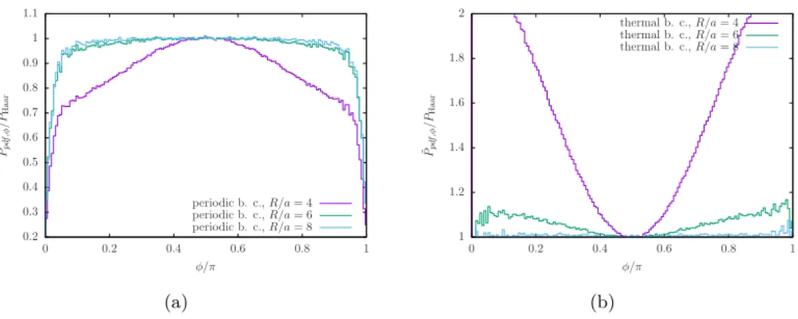
the Haar measure has to be considered as an important contribution in the lattice simula- tions. In our numerical studies, we use the distribution of the per-site Polyakov loop phase φ normalized with respect to the Haar measure for different R to gain a sense of distinction between Abelian and non-Abelian confinement regimes.

The picture that emerges by the examination of the thermal and graded partition functions corresponding to thermal and periodic compactification with analytic (lattice perturbation theory at weak coupling domain) and numerical (both at weak and strong coupling domain) methods is as follows: at low temperatures or large-circle size R where the theory becomes strongly coupled, there are rather unconstrained fluctuations of the φ ab , which leads to a vanishing Polyakov line expectation value. At higher temperatures, or small circles, the weak coupling at the scale of the circle size admits a calculable poten- tial for the Polyakov loop, which may lead to either to a confined or deconfined vacuum depending on the details. The Polyakov line expectation value is in this case determined by the minimum of the effective potential of φ _ab and the randomness of the fluctuations be- comes suppressed, regardless of whether the theory is confined or deconfined. However, the suppression of the randomness of fluctuations will happen in different ways: in the thermal deconfined phase, there is a dominance of the φ = 0 center-broken configuration, in the periodic confined phase, a dominance of the φ = ^π ₂ center-symmetric configuration. The center-symmetric suppression of the randomness of fluctuations is a signal of the dynamical abelianization according to the Abelian confinement picture. The confinement that takes place at large-circle (strong renormalized coupling) is referred to as non-Abelian confine- ment picture. In the present work, we provide evidence for the continuity between the two.

It is worth mentioning that historically well-known examples of Abelian confine- ment mechanisms such as the three-dimensional Polyakov model [1] and the softly broken Seiberg-Witten theory in four dimensions [42]. These theories have a property which is unlike pure Yang-Mills theory. In pure Yang-Mills theory, k-string tensions are classified by N c -ality. There is only one-type of string between a quark with N c -ality k and its anti-quark with tension T _k . Consider for example the 1-string tension T ₁ . However, in the above mentioned theories, since the gauge group is U(1) ^N

⁻¹ and since the Weyl sym- metry permuting gauge group factors are spontaneously broken, T 1 is replaced by N c − 1 fundamental strings, T _1,j as shown in [44]. This is not the case in QCD(adj) as well as deformed Yang-Mills theory, where the Z N

sub-group of the Weyl group remains intact in the Abelian confinement regime. Consequently, there is again only one-type of fundamental string, see [45] for details.

4.2 Different Polyakov line effective actions

A deep understanding of the different non-perturbative definitions of the Polyakov line effective action is required to link lattice results to the one-loop perturbative calculations.

There is a difference between the effective action for the Polyakov loop P _L and the one

of φ _a . These two effective actions are related for a constant background by the Fourier

representation of eq. (4.16), but there is no general identification between the expectation

values hP _L i and hφ _a i. We won’t enter the discussion about the convexity of the effective

action since it is not relevant for our discussions, see [46] for further details.

JHEP11(2018)092

The relevant counterpart of the effective action that is easily accessible on the lattice is the constraint effective potential, see [46–48] for a discussion. Up to an overall constant, it is the logarithm of the probability density of the observable O

V _c (Φ) = − 1 V log

Z

Dθ δ(Φ − O(θ))e ^−S[θ]

= − log [P _{pdf ,O} (Φ)] + constant . (4.21) The integration variable θ represents all gauge and fermion fields. The probability density P pdf,O (Φ) can be numerically approximated by the histogram of O obtained from the Monte-Carlo data. The most relevant information can be already extracted from the lowest moments of the distribution. A crucial role is played by the second moment which is equivalent to the susceptibility of eq. (3.3). The susceptibility is the inverse of the coefficient in front of the quadratic term in the effective potential.

The definition (4.21) shows that the identification of the phase to the Polyakov line effective potential in eq. (4.16) is unambiguous only in the constant field limit. In the general case, the Polyakov line eigenvalues and the phases are space-dependent. The φ a

in the effective potential can be identified with the volume averaged phase factors or the phases of the volume averaged Wilson lines. In both cases the direct application of the perturbative formulas is not possible since either the volume averaged loop can not be determined from the volume average phases, or the volume averaged Wilson line is not a group element. A qualitative agreement with the potential of eq. (4.16) is still expected, especially in the strong and weak coupling limit where the fluctuations of the phase factors are suppressed.

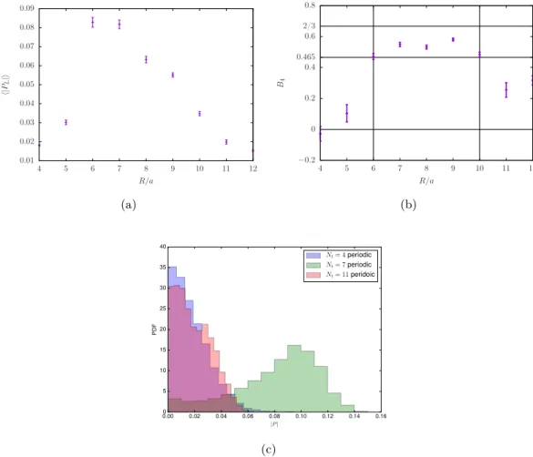
A constraint effective potential can also be defined from the per-site distribution of the observable. This distribution can be determined with a better accuracy due to the additional volume factor in the statistical sampling. The per-site distribution is significantly different from the distribution of the volume averaged observable. Smoothing techniques of the field configuration can be applied in order to match the two distributions, but still the infinite volume limit is not well defined for the per-site distribution. In the strong coupling limit the per-site constraint effective potential agrees with the constraint effective potential of the Polyakov line. This leads to the several different definitions of the Polyakov line effective potential mentioned in the literature: the Polyakov line effective potential, the per-site Polyakov line effective potential and the same for the effective potential of φ a . The per-site distribution has been investigated in particular to confirm the non-Abelian confinement. As explained above, the contributions of the Haar measure have to be fac- torized out in order make contact to this view of the confinement mechanism. Such an analysis has been done in [39] for the case of SU(3) QCD(adj) with N f > 1 and we perform a similar analysis here for SU(2) SYM. In addition, we discuss the susceptibility in order to get information about the form of the effective action from the numerical simulations.

5 The phase diagram on the continuum and lattice

Below, we review the phase diagram of N = 1 SYM and QCD(adj) with periodic boundary

condition on R ³ ×S ¹ . Part of these phase diagrams are calculable by weak coupling methods

JHEP11(2018)092

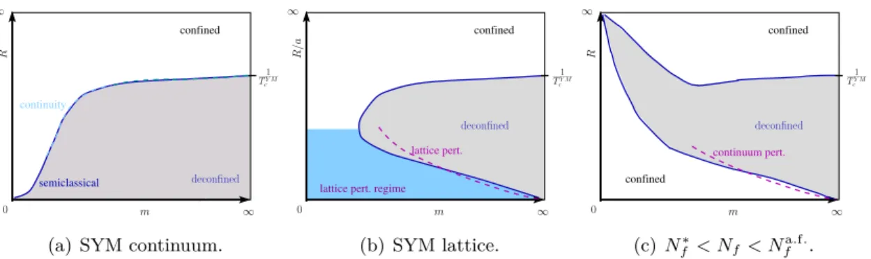
confined

continuity

semiclassical

∞

0 m ∞

R

T_c1^{Y M}

deconfined

(a) SYM continuum.

confined

lattice pert. regime lattice pert.

∞

0 m ∞

R/a

T_c1^{Y M}

deconfined

(b) SYM lattice.

confined

confined

continuum pert.

∞

0 m ∞

R

T_c^{Y M}1

deconfined

(c) N

< N

< N

.

Figure 2. A sketch of the expected phase diagrams in N f QCD(adj). Figure (a) is the continuum case in SYM with the semiclassical predictions valid on the small (R, m) corner, the well established numerical results at large-m (where semi-classic does not apply) and the conjectured continuity of the transition line. Figure (b) is the phase diagram of SYM on the lattice at a fixed lattice spacing.

At small R/a regime the transition line approaches lattice perturbation theory. The “lattice pert.

regime” corresponds to a region where the coupling stays small at the scale of compactification.

There are crucial discretization effects in this regime. In this regime the theory behaves similar to continuum QCD(adj) with larger N f . (Figure (c)) If N _f ^∗ < N f < N _f ^a.f. becomes larger than a certain critical value dictated by lower end of conformal window and smaller than asymptotic freedom bound, the theory on decompactification limit is a CFT. However, upon compactification (with periodic boundary conditions), center is stable and confinement sets in. Continuum one-loop perturbative analysis can be used to show that R c m = 3.484 for N f = 5 (lower transition line).

The upper transition line is non-perturbative and not calculable.

involving a combination of perturbative one-loop effective potential for Wilson line and non-perturbative semi-classical methods.

Next, we describe the calculable critical compactification radius R c as a function of N _f and m ₀ by using the one-loop effective potential on the lattice. We also briefly review the part of the phase diagram that is accessible by lattice techniques, but not via weak coupling methods.

Continuum, N _f = 1 QCD(adj): the phase diagram of N = 1 SYM in the continuum is shown in figure 2(a). The small (m, R) corner of this phase diagram is semi-classically calculable and exhibits a center-symmetry changing phase transition due to asymptotic freedom and unbroken center symmetry in the chiral limit [19, 38]. In the large-m regime, the theory approaches pure Yang-Mills theory as fermions decouple. This regime is not semi-classically calculable, but from lattice simulations, it is known that a transition exists and it is natural to expect that the transition line extrapolates from small m to large-m regime. In this picture, there is only one transition line from confined to deconfined phase.

The theory is non-perturbatively confined for all m < m c or R > R c in the calculable limit with a transition boundary at [19]

R _c = Λ ⁻¹ r m

8Λ for N _f = 1 (5.1)

where Λ is the strong scale.

JHEP11(2018)092

There are two conjectural continuities in the phase diagram shown in figure 2(a) cor- responding to the twisted partition function (1.1):

• Adiabatic continuity between the small-R weak coupling confined phase and large-R regime where the theory becomes strongly coupled at large distances.

• The continuity of semiclassical (weak coupling) and the strong coupling phase tran- sition.

There is a sufficiently strong reason to believe continuity if the fermion mass is zero. (1.1) reduces to the supersymmetric Witten index [18] at m = 0,

I W = ˜ Z(R, m = 0) = tr ^h e ^{−R H ˆ (0)} (−1) ^{F i} = N c for SU(N c ), (5.2) which counts the difference of bosonic and fermionic ground states. At fixed small-m, for R < R c , one can prove the stability of the confined phase, and also prove the existence of center symmetry breaking for R < R _c [19]. The main aim of the present work is to find a non-perturbative evidence for the above adiabatic continuity conjectures.

1 < N _f < N _f ^a.f. QCD(adj): let us first recall the conjectured phase diagram of QCD(adj) in the continuum. Let N _f ^∗ denote the putative number of flavors below which the theory is confining and above which it exhibits IR-conformality on R ⁴ . For N _f ≥ N _f ^a.f.

even asymptotic freedom is lost.

The expected phase diagram for 1 < N _f < N _f ^∗ is the same as shown in figure 2(b) and for N _f ^∗ < N _f < N _f ^a.f. , it is shown in figure 2(c). In both of these diagrams, the upper transition lines are incalculable by weak coupling methods but the lower lines are calculable.

The one-loop potential is of the form:

V ^pert. (φ) = N ²

∞

X

n=1

V _n P _L ^{(n) 2} , V _n = 4 π ² n ⁴

−1 + N _f

2 (nRm) ² K ₂ (nRm)

. (5.3) Even at very large-m, as one dials R, it is possible to show that V ₁ is positive for R < R c

and center symmetry is stable. V ₁ is negative for R _c < R . Λ. This calculable phase transition correspond to the lower lines in figures 2(b) and 2(c). The lower phase boundary for SU(2) N _f flavor QCD(adj) for any N _f < N _f ^a.f is given by [38]

m c R ^cont. _c = {2.027, 2.709, 3.154, 3.484} for N f = 2, 3, 4, 5. (5.4)

The interesting aspect of the phase diagram is the non-decoupling of heavy fermions

once the circle size is taken sufficiently small. In that regime, the fermion, despite being

heavy, enters in the combination mR and a sufficiently small R makes the fermions behave

as if they were light in that regime. The upper lines in these figures are incalculable by

weak coupling methods, but it is essentially the deconfinement radius of pure Yang-Mills

theory because massive fermions decouple in that regime.

JHEP11(2018)092

0 2 4 6 8 10 12

0 0.5 1 1.5 2 2.5

Rc/a

m0

Nf= 1 Nf= 2 Nf= 3 Nf= 4

(a) Phase transition.

0 0.5 1 1.5 2 2.5

0 0.05 0.1 0.15 0.2 0.25 0.3

a(mc)LAT−amc

a/R Nf= 1

Nf= 2 Nf= 3 Nf= 4

(b) Continuum limit.

0 0.5 1 1.5 2 2.5 3 3.5 4 4.5

4 6 8 10 12 14 16

Rcmc

R/a

latticeNf= 1 continuumNf= 2 continuumNf= 3 continuumNf= 4

(c) Transition as function of R/a.

Figure 3. Figure (a): numerical determination of the critical radius R c for the deconfinement transition as a function of the mass in the one-loop approximation on the lattice from eq. (4.14) for N _f QCD(adj). In figure (b) the deviations of the critical mass (m _c ) _LAT determined by the one-loop lattice effective potential from the expected continuum result m c (eq. (5.4)) are represented as a function of a/R. Keeping R fixed, the difference tends to zero in the continuum limit. Figure (c) represents the transition for N _f = 1 as a function of R/a to compare R _c m _c with the values of eq. (5.4).

Lattice: the expected deconfined regions on the lattice are shown for different N _f in figure 3(a). Even for N _f = 1, there is a perturbative transition line since lattice artefacts violate the exact cancellation between gluon and fermion loops, especially at scales close to the lattice cutoff 1/a. Such a significant deviation from the continuum phase diagram is expected for small R/a, while in the large R/a regime a good agreement with the continuum predictions should be observed. The corresponding convergence to the continuum limit is shown in figure 3(b). The deviations from the continuum phase diagram at m ₀ > 0 and small R/a are labeled as the “lattice pert. regime” in figure 2(b). In this regime the theory behaves rather similarly to QCD(adj) for N _f > 1 in the continuum with a confined phase that extends up to larger m the smaller R/a is. The appearance of this regime is in agreement with the result of our first numerical simulations [29].

The coefficient V _eff ⁽ⁿ⁾ in the perturbative effective Polyakov loop potential of SYM pro- vides some further indications for the difference between lattice and continuum phases:

the numerical solution shows that it monotonically decreases with R/a. In the continuum

V _eff ⁽ⁿ⁾ = 0 at the perturbative level and due to the non-perturbative contributions it be-

JHEP11(2018)092

comes an increasing function of R. There is hence a competition between non-perturbative effects and perturbative lattice artefacts: the transition to the “lattice pert. regime” is in- dicated by a turnover from the increasing continuum to the decreasing lattice perturbative behaviour, a minimum of V _eff ⁽ⁿ⁾ and a maximum of the susceptibility. The investigation of the continuity in SYM is limited to a certain range of R/a before this turnover, where the lattice artefacts are under control. This is the limit of large R/a while R is kept small.

Even outside this regime, the qualitative properties are not completely different. They can be compared to N _f > 1 QCD(adj) in the continuum and the qualitative features should be similar.

The perturbative continuum regime is reached considering the limits β → ∞ and R/a → ∞, the continuum limit for an asymptotically free theory regularized on the lattice.

In this limit there is a simple perturbative relation between the renormalized mass m and the bare mass in lattice units m ₀ . A regime where the perturbative effective potential provides a reasonable approximation is also approached in the small R/a limit at fixed lattice spacing. However, this is not strictly perturbative, in particular a non-perturbative renormalization of the mass is required. The mass parameter m ₀ in the perturbative formulas is replaced by m/a fixed by some renormalization condition, in our case a fixed value of the adjoint pion mass in the large R limit. The fixed scale approach that we apply in our current study allows to keep the line of constant physics, i. e. constant renormalized parameters, unambiguously, compared to our previous studies in [29].

5.1 Explanation of the discrepancy of lattice and continuum

The phase diagram of lattice SYM with Wilson fermions and Wilson parameter set to r = 1 exhibits a different phase structure than in the continuum limit. In particular, for sufficiently small-bare mass, the lattice theory is always confined and for a large mass, it is confining at large R, deconfined in an intermediate regime, and confined again at small-R, as shown in figure 2(b). Note that the lattice regularization neither respects supersymmetry, nor chiral symmetry. In fact, if it were to respect one, it would respect the other as the only relevant chiral symmetry breaking operator m λλ ¯ is also the only supersymmetry breaking relevant operator for this system.

Here, we explain this discrepancy in more detail, and argue that both of these conclu- sions are actually correct, and that there is no contradiction between the two results.

Recall that both the continuum and lattice study aim to understand phase structure of the theory by using

Z(R, m) = tr ˜ ^h e ^{−R H(m) ˆ} (−1) ^{F i} (5.5) In continuum, for m = 0, ˜ Z(R, 0) is the supersymmetric Witten index, independent of R.

Hence, there is no phase transition on the m = 0 axis for any value of R. In the small-R regime, there is no perturbatively induced potential for Wilson line.

There are non-perturbative monopole-instantons with two fermion zero modes M _a =

e ^−S

e ^{−~ α}

^{·( φ−i~ ~ σ)} (~ α a λ) ² where φ ~ is the holonomy field and ~ σ is the dual photon. The crucial

point is that despite the fact that monopole-instanton couple to holonomy field, it does

not induce a boson potential as it has fermion zero modes. Rather, it does induce a chiral