Double Parton Distributions

Double Parton Distributions

Perturbative splitting, sum rules, and models

Dissertation zur Erlangung

des Doktorgrades der Naturwissenschaften (Dr. rer. nat.) der Fakult¨ at f¨ ur Physik der Universit¨ at Regensburg

vorgelegt von

Peter Pl¨oßl

aus Nabburg

im Jahr 2019

Promotion angeleitet von: Prof. Dr. Andreas Sch¨afer

Pr ¨ufungsausschuß: Dr. Markus Diehl Prof. Dr. Jascha Repp Dr. Juan Diego Urbina Datum der m ¨undlichen Pr ¨ufung: 23.07.2019

Acknowledgements

As this thesis would not have been possible in its present form without the support from a number of people, I want to express my gratitude for this. First of all I would like to thank my supervisor, Professor Andreas Sch¨afer, who sparked my interest in high energy physics with an extensive lecture on theoretical and experimental particle physics. As a result of this I joined his group for my Bachelor’s thesis and stayed throughout my Master’s degree and finally for my PhD.

For my Master’s thesis I started working on multiple partonic interactions (MPIs) in collaboration with Markus Diehl and Jonathan Gaunt who have been collaborators from this day on. For this I would like to thank them, as they took their time to explain many of the subtleties encountered in perturbative QCD in general and MPIs in particular.

Markus Diehl was basically my second supervisor during my PhD and always had extremely valuable input whenever I was stuck with a problem. Collaborating with Jonathan Gaunt for the final project of my PhD greatly improved my understanding of perturbative QCD calculations, for which I am very grateful. I would also like to thank Daniel Lang who worked with me on the sum rule improved DPD models and helped quite a lot with the numerical implementation.

For the great times during numerous lunch and coffee breaks I would like to thank my fellow graduate students, many of whom became close friends over the course of the years. In particular I am thankful to Jakob Simeth and Max Emmerich with whom I shared an office. At this point it should not go unmentioned that also many of my close friends supported me in one way or another, for which I am very grateful.

And finally, last but not least, I would like to thank my family – my parents, my sister, and my grandma – for being supportive of me in every way possible for so many years.

Without them and their continued support I probably would have given up somewhere

along the way.

Abstract

The overarching topic of this thesis is double parton scattering (DPS), which describes the situation when two individual hard scattering reactions occur in a single hadron- hadron collision. In some regions of phase space DPS may give sizeable contributions to the production of multi-particle final states and thus be an important background to single parton scattering (SPS). Not only this, but DPS is also an interesting phenomena in its own right, as it gives insight into the correlations of partons inside of hadrons.

Therefore a theoretical description of such processes from first principles is required.

Such a prescription is obtained in the form of a factorisation theorem akin to the one known from SPS, with a central building block being the double parton distributions (DPDs). However, these DPDs are presently basically unknown as experimental data is still lacking.

One of the few general theoretical constraints for DPDs are the number and momentum sum rules proposed by Gaunt and Stirling. In chapter 3 of this thesis a proof is presented that the DPD sum rules are valid at all orders in the strong coupling for renormalised distributions. As by-products of this proof the all order form of the inhomogeneous evolution equation for momentum space DPDs can be derived and it can be shown how the inhomogeneous term in this equation is related to the contribution of a short distance 1 ! 2 splitting to the DPDs. It can furthermore be shown that the 1 ! ² evolution kernels in the inhomogeneous term fulfil number and momentum sum rules closely resembling the ones for DPDs.

In chapter 4 the sum rules considered in chapter 3 are used to construct improved position space DPD models. To this end it is first shown how position space DPDs can be matched onto the momentum space DPDs for which the sum rules have been shown to be valid. Following this an initial DPD model consisting of an intrinsic part and a contribution from the perturbative 1 ! 2 splitting is iteratively refined in order to obtain the best possible agreement with the DPD sum rules. In particular, this highlighted that a good agreement with the momentum and equal flavour number sum rules is not possible without taking into account the 1 ! 2 splitting contribution.

Finally the dependence of the agreement with the sum rules on the renormalisation scale and the cut-off scale introduced by the matching onto momentum space DPDs is investigated.

As the 1 ! 2 splitting contribution has been shown to be quite important for DPS it is

extensively studied in chapter 5. In particular, the next-to-leading order (NLO) expres-

sion for this splitting is the only missing quantity required for NLO DPS calculations.

colour singlet DPDs in all partonic channels using state of the art techniques. From this

momentum and position space 1 ! 2 splitting kernels as well as the 1 ! 2 evolution

kernels needed in the inhomogeneous evolution equation of momentum space DPDs

are extracted at NLO. As a cross-check for the correctness of the results the agreement

of the 1 ! 2 evolution kernels with the sum rules derived in chapter 3 is explicitly

verified. Finally various kinematic limits of the momentum space splitting kernels and

the evolution kernels are discussed.

Contents

Abstract v

1. Introduction 1

2. Theory 5

2.1. Quantum ChromoDynamics . . . . 5

2.1.1. A brief history of QCD . . . . 5

2.1.2. Renormalisation and the running coupling . . . . 8

2.1.3. Factorisation theorems: the backbone of perturbative QCD . . . 11

2.2. General double parton scattering theory . . . . 15

2.2.1. Factorisation for double parton scattering . . . . 16

2.2.2. Double parton distributions . . . . 18

Definition of bare PDFs and DPDs . . . . 18

Renormalisation and evolution of DPDs . . . . 21

2.2.3. A consistent framework for double parton scattering . . . . 28

3. DPD sum rules in QCD 31

3.1. Introduction . . . . 31

3.2. Specific Theory . . . . 32

3.2.1. The DPD sum rules . . . . 33

3.2.2. Light-cone perturbation theory . . . . 34

3.3. Analysis of low-order graphs and its limitations . . . . 36

3.3.1. Sum rules with a gluon PDF . . . . 36

3.3.2. Sum rules with a quark PDF . . . . 41

3.4. All order proof for bare distributions using LCPT . . . . 44

3.4.1. Representation of PDFs and DPDs in LCPT . . . . 44

3.4.2. All order correspondence between PDF and DPD graphs . . . . 47

3.4.3. Number sum rule . . . . 49

3.4.4. Momentum sum rule . . . . 50

3.5. Validity of the sum rules after renormalisation . . . . 51

3.5.1. Implementation of the MS scheme. . . . 51

3.5.2. Number sum rule . . . . 53

3.5.3. Momentum sum rule . . . . 55

3.6. DPD evolution and its consequences . . . . 57

4. Sum rule improved position space DPD models 63

4.1. Introduction . . . . 63

4.2. Specific theory . . . . 64

4.2.1. From position space DPD models to

= 0 momentum space DPDs 64 4.2.2. Initial DPD model . . . . 65

4.2.3. Technical details and numerics . . . . 68

4.3. Refining the DPD model . . . . 71

4.3.1. Initial DPD model . . . . 71

4.3.2. Modified phase space factor and number effect subtractions . . . 75

4.3.3. Fine tuning the modified phase space factor . . . . 76

4.3.4. Modifying the splitting contribution . . . . 80

4.4. Scale dependence of the sum rules . . . . 88

4.4.1. Renormalisation scale dependence . . . . 88

4.4.2. Cut-off scale dependence . . . . 90

5. Two-loop splitting in double parton distributions 95

5.1. Introduction . . . . 95

5.2. Specific Theory . . . . 96

5.2.1. Reduction to master integrals: integration by parts reduction . . 96

5.2.2. Calculating master integrals: method of differential equations and the canonical basis . . . . 98

5.3. Renormalisation Group analysis: Splitting kernels at higher orders . . . 100

5.3.1. Preliminaries . . . . 101

MS implementation and coupling renormalisation . . . . 101

Renormalisation factors and splitting functions . . . . 102

5.3.2. Momentum space kernels . . . . 103

Equivalence of MS scheme implementations . . . . 106

5.3.3. Position space kernels . . . . 106

Higher orders . . . . 108

5.4. Matching between momentum and position space DPDs at higher orders 109 5.4.1. Matching at zero

. . . . 110

Higher orders . . . . 112

5.4.2. Matching at non-zero

. . . . 112

5.4.3. Scale independence of matching . . . . 114

5.5. Two-loop calculation . . . . 116

5.5.1. Channels and graphs . . . . 116

5.5.2. Performing the calculation . . . . 122

Real emission diagrams . . . . 123

Virtual diagrams . . . . 128

5.6. Results . . . . 128

5.6.1. Support and singularity structure . . . . 129

5.6.2. 1 ! 2 evolution kernels . . . . 130

Contents

5.6.3. 1 ! 2 momentum space splitting kernels . . . . 134

Terms originating from LO kernels . . . . 135

Non-logarithmic terms . . . . 136

5.6.4. Number and momentum sum rules . . . . 138

Number sum rule . . . . 138

Momentum sum rule . . . . 139

5.6.5. Active-spectator symmetry . . . . 139

5.6.6. Kinematic limits . . . . 140

Threshold limit: large x

+ x

. . . . 141

Small x

+ x

. . . . 142

Triple Regge limit . . . . 144

Small x

or x

. . . . 146

6. Summary and Outlook 149 A. Feynman rules 155

A.1. Scalar Feynman rules in light-cone gauge . . . . 155

A.2. QCD Feynman rules . . . . 155

A.2.1. Feynman gauge . . . . 156

A.2.2. Light-cone gauge . . . . 157

Bibliography 161

List of Figures

2.1. General structure of the Drell-Yan process . . . . 12

2.2. Leading subgraphs for the Drell-Yan process . . . . 13

2.3. Factorised TMD Drell-Yan cross section . . . . 15

2.4. Leading subgraphs for the double Drell-Yan process . . . . 16

2.5. Factorised TMD double Drell-Yan cross section . . . . 17

2.6. Assignment of position and momentum arguments in DPDs . . . . 18

2.7. 1-v-1 and 2-v-2 contributions to the DPS cross section . . . . 29

3.1. Order O (

) gluon PDF graphs . . . . 36

3.2. Transition from a PDF to a DPD graph . . . . 37

3.3. Order O (

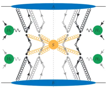
) gluon-quark and gluon-antiquark DPD graphs . . . . 38

3.4. Order O (

) real emission quark PDF graphs . . . . 42

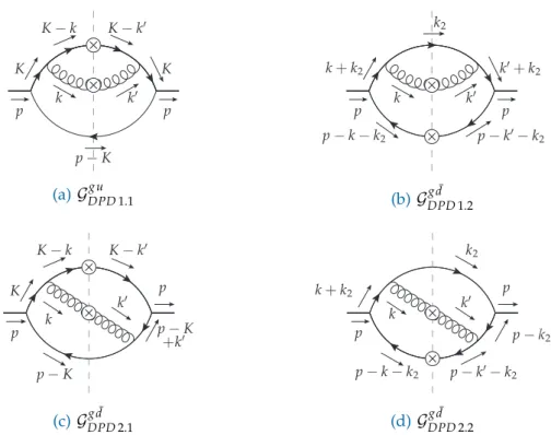
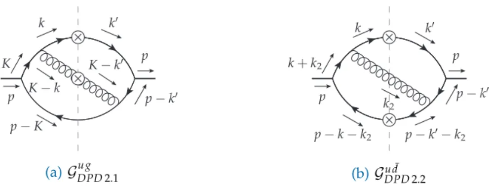
3.5. Order O (

) ug and u d ¯ DPD graphs . . . . 42

3.6. Schematic illustration of an LCPT graph for a PDF . . . . 46

3.7. LCPT graphs for a PDF or a DPD . . . . 48

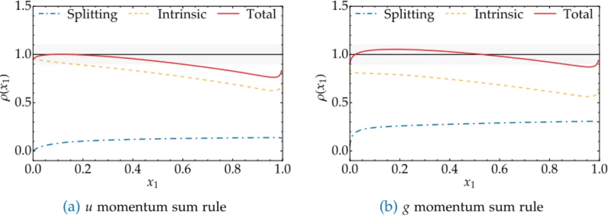
4.1. g and u momentum sum rule ratios for the initial model . . . . 72

4.2. Different powers of the phase space factor . . . . 73

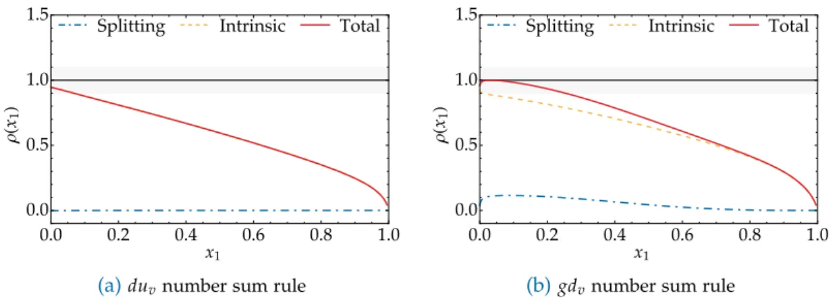
4.3. Mixed flavour number sum rules ratios for the initial model . . . . 74

4.4. Equal flavour number sum rules ratios for the initial model . . . . 74

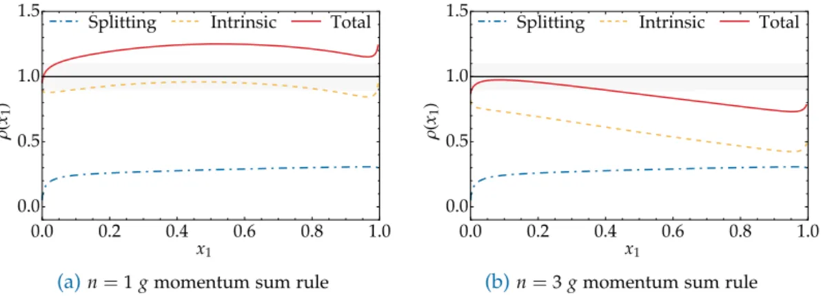
4.5. g and u momentum sum rule ratios after the first iteration . . . . 76

4.6. Equal and mixed flavour number sum rule ratios after the first iteration 76 4.7. Illustration of the average deviations per sum rule . . . . 78

4.8. g and u momentum sum rule ratios after the second iteration . . . . 78

4.9. Difference between the number sum rule ratios for the first and second iteration . . . . 79

4.10. Modification functions g

for the individual g ! ^{q q ¯} splittings . . . . . 84

4.11. Effect of the splitting modification on the equal flavour number sum rules 85 4.12. Effect of the g ! ^{q q ¯} modification on the quark momentum sum rules . 86 4.13. Effect of the q ! ^qg modification on the quark momentum sum rules . 86 4.14. Effect of the g ! ^gg modification on the gluon momentum sum rule . . 87

4.15. Quark momentum sum rules at different scales . . . . 88

4.16. Equal flavour number sum rules at different scales . . . . 89

4.17. gq

number sum rules at different scales . . . . 90

4.18. Equal flavour number sum rules at different scales . . . . 90

4.19. Cut-off scale dependence of the momentum sum rules in the initial model 91

4.20. Cut-off scale dependence of the equal flavour number sum rules in the

initial model . . . . 92

4.21. Cut-off scale dependence of the momentum sum rules in the initial model 92 4.22. Cut-off scale dependence of the equal flavour number sum rules in the final model . . . . 93

5.1. Real graphs for LO channels . . . . 118

5.2. Real graphs for NLO channels . . . . 119

5.3. Virtual graphs for LO channels . . . . 120

5.4. Rules for obtaining Wilson line graphs from graphs without Wilson lines 121 5.5. Assignment of transverse momenta in of a real graph . . . . 122

5.6. Assignment of momenta in generic virtual graphs . . . . 122

A.1. Scalar Feynman rules in light-cone gauge . . . . 157

A.2. QCD Feynman rules in Feynman gauge . . . . 158

A.3. Ghost Feynman rules in Feynman gauge . . . . 159

A.4. QCD Feynman rules involving eikonal lines in Feynman gauge . . . . . 159

A.5. Feynman rules for gluon distributions . . . . 160

1. Introduction

One of the great successes of physics in the 20

century was the establishment of the Standard Model of particle physics (SM) as the theory of the known microscopic interactions in a combined effort of theoretical and experimental particle physicists.

Within the framework now known as the SM the interactions of elementary particles via the fundamental forces are on one hand described by the electroweak theory which is a unification of the theories describing the electromagnetic interaction – Quantum ElectroDynamics (QED) – and the weak interaction – Quantum FlavourDynamics (QFD) – responsible for radioactive decays, and on the other hand by the theory of strong interactions – Quantum ChromoDynamics (QCD) – governing how quarks interact to form hadrons, while gravitation is completely neglected in the SM. Incorporating a quantum theory of gravitation that is compatible with general relativity into the SM is one of the most important steps towards a unified description of the fundamental interactions. Nevertheless, even without this

the SM has proven remarkably successful in predicting experimental results, with its latest and probably best known (at least to the general public) success being the discovery of the Higgs boson at the Large Hadron Collider (LHC). The existence of this elusive particle had been predicted already in the 1960’s as a fundamental building block of the SM and its experimental observation was celebrated as the completion of the SM. However, the failure to account for the effects of gravitation is not the only weakness of the SM as it also fails to explain the observed matter-antimatter asymmetry as well as the existence of dark matter and dark energy. Phenomena associated with these – and other – things not explained by the SM are referred to as beyond Standard Model (BSM) physics and are a very active field of research within the particle physics community with great experimental efforts invested in the observation of such phenomena. Despite this so far no direct evidence of BSM physics has been detected, suggesting that deviations from the SM predictions are – at currently accessible energies – very small. This implies that not only increased experimental accuracy and higher collision energies are required in order to discover BSM effects, but also the precision of theoretical predictions has to be pushed further.

Currently the largest uncertainties are associated with predictions regarding the strong interaction, on one hand due to the fact that the coupling constant of the strong interaction is comparably large, and on the other hand because calculations within QCD tend to be quite a bit more involved than for example in QED such that calculations of higher order terms in the perturbative expansion tend to become cumbersome. Besides

1The reason for this is that at the energies – and thus also distances – probed at present day colliders gravitation can be neglected compared to the other fundamental forces.

this, most QCD calculations and event generators only take leading power contributions into account while the full plethora of possible (power suppressed) QCD effects is not taken into account in a systematic manner. One example are so called multiple partonic interactions (MPIs) which can contribute to the production of multiple hard final states.

Consider to this end the simplest MPI reaction, namely double parton scattering (DPS), which is also the largest of the MPI contributions. The typical assumption in hadron- hadron collisions is that the final state with an associated hard scale Q is produced in a single parton scattering (SPS) event where one parton from one of the colliding hadrons scatters of a single parton in the second colliding hadron, while the remaining partons do not partake in any hard scatterings and fly off as beam remnants. In the case that the final state can be divided into two subsets A and B with associated hard scales Q

and Q

the final states can furthermore be produced by so called double parton scattering (DPS) events where two partons from each colliding hadron enter distinct hard scatterings. Experimental evidence of DPS has already been found in the 1980’s and 1990’s as can be seen in references [1–5] and also more recently at the LHC as evidenced by the results in references [6–18]. In particular it is expected that especially after the rather recent energy upgrade at the LHC and even more so at possible future higher energy hadron colliders the rate of MPI events will further increase as will be discussed in a bit. A generalisation of the situation with two distinct subsets in the final state to the case of multiple distinct subsets in the final state which can be produced by MPIs arises naturally following the rationale for DPS above. However, when integrated cross sections are considered already DPS is is power suppressed compared to SPS by

/Q

where

is a generic hadronic scale while Q is the smaller of the two hard scales Q

and Q

. Despite of this suppression DPS can nevertheless compete with SPS in some cases where the production of the final states via SPS involves small coupling constants or higher orders in the coupling constant, with the most well known of these probably being the production of a same sign WW pair as described in references [19–24]. When cross sections differential in the transverse momenta of the final states are considered it has been shown in references [25–28]

that for small transverse momenta of the final states DPS contributes at leading power, comparable to the SPS contributions. In references [29–31] is has furthermore been pointed out that DPS gives sizeable contributions to the overall cross sections in the case of a large rapidity separation between the two subsets A and B in the final state.

As mentioned above, the relative importance of DPS compared to SPS is expected

increase with increasing collision energy. This can be understood if one considers that

on one hand with increasing collision energy smaller and smaller momentum fractions

of the constituent partons are probed while on the other hand the DPS cross section is

expected to scale like the fourth power of a parton distribution whereas SPS scales like

the second power of a parton distribution. Since parton distributions exhibit a strong

growth for small momentum fractions this leads to an enhancement of DPS relative to

SPS. While the inclusion of MPIs and in particular DPS in perturbative cross section

calculations is required in order to improve theoretical precision, MPIs are interesting

to study in their own right, as they give access to a detail picture of hadron structure

that is not accessible in SPS reactions. In particular the study of MPI processes makes it possible to obtain information about correlations between the partons making up hadrons as well as their distribution in transverse momentum space.

A systematic description of MPIs from first principles requires the extension of the well- known SPS factorisation theorems to the case of multiple hard interactions, giving rise to multi parton distributions in close analogy to the regular single parton distributions (PDFs). First steps in this direction were already taken in the 1980’s when physicists first gained interest in MPIs as evidenced by references [32, 33] and a more stringent theoretical treatment was developed more recently with a particular focus on DPS as this is naturally the leading of the MPI contributions. In recent years quite some progress has been made towards a complete proof of factorisation for DPS in close analogy to the proofs of SPS factorisation theorems, especially in references [26, 34–36]. Furthermore a framework has been developed in reference [35] that allows for a clean separation of SPS and DPS contributions in regions of phase space where they overlap. At this point the theoretical framework for DPS calculations – even at higher orders – has reached a level of sophistication comparable to the SPS factorisation theorems. Nevertheless it is still not quite possible to perform DPS cross section calculations from first principles as a crucial ingredient in the DPS factorisation formula is still missing – the double parton distributions (DPDs) which contain the non-perturbative part of the full DPS cross section. As these DPDs are genuine nonperturbative quantities they cannot be calculated in perturbation theory and either have to be obtained from experimental data or using nonperturbative methods like lattice computations. Since DPS signals are generally small compared to the SPS case and an experimental determination of DPDs requires huge amounts of data the former is not possible at present and even though quite a lot of progress has been made regarding the extraction of parton distributions from lattice data the situation for DPDs is not as favourable there either.

In order to still be able to compute DPS cross sections many physicists resort to what

is known as the DPS pocket formula in which the DPS cross section is factorised into

a product of SPS cross sections divided by a so called effective cross section. Such a

factorised form of the DPS cross section arises when DPDs are approximated by simple

products of PDFs multiplied by a spatial profile function, neglecting even the most

basic correlations of the partons inside a hadron. A possible way to do better than

this approach is to construct more sophisticated DPD models incorporating at least

the most basic correlations. To this end any type of constraint placed upon the DPD

models is valuable input and one possible constraint is the behaviour of the DPDs

at small transverse separation between the two partons. In this regime the DPDs are

dominated by what is referred to as the 1 ! 2 splitting contribution in which the two

partons arise from a short-distance splitting of a single parton. In this limit the DPDs

can be expressed in terms of a convolution of perturbative 1 ! 2 splitting kernels and

regular PDFs. This 1 ! 2 splitting contribution and its effect an DPDs and the DPS

cross section has already been studied extensively in references [25, 26, 28, 35, 37–44]. A

second kind of constraint was proposed by Gaunt and Stirling in reference [45] in the

form of sum rules corresponding to the conservation of quark flavour and momentum

which momentum space DPDs have to fulfil, reaffirming the interpretation of DPDs as probability densities.

The main aim of this thesis is to gain a better understanding how to model DPDs in a way that most closely resembles the physical reality. To this end first a brief review of the underlying theory of QCD is presented in section 2.1 followed by an overview over the more specific DPS theory in section 2.2 where first the derivation of factorisation theorems for DPS is discussed in section 2.2.1 before definitions and properties of DPDs are addressed in section 2.2.2. In their original work on the DPD sum rules Gaunt and Stirling noted that the sum rules remain valid under LO renormalisation group evolution, given that they are fulfilled at the initial renormalisation scale. As the DPD sum rules provide one of the only constraints placed on DPDs it is of utmost importance to make sure that they are indeed valid in QCD at any scale. A first proof of this using light-cone wave functions was given in appendix C of reference [46]. However, while the framework of light-cone wave functions allows to keep track of kinematic and combinatorial factors, basically recovering the probabilistic parton model interpretation, the subtleties of renormalisation have not been fully taken into account in the proof presented in reference [46]. In chapter 3 this will be rectified by a detailed analysis of the UV singularities in DPDs and the effect of renormalisation on the validity of the sum rules. In particular it will be shown that the sum rules are indeed valid for renormalised DPDs to all orders in perturbation theory. Following this analysis the sum rules – together with the LO expression for the perturbative 1 ! 2 splitting contribution to DPDs – will be used in chapter 4 to construct a sum rule improved position space DPD model. To this end the model suggested in reference [35] is used as a starting point for iterative refinement of this model with help of the sum rules. Following this a calculation of the 1 ! 2 splitting contribution at NLO will be presented in chapter 5.

The results obtained there are the last missing step towards NLO DPD models and

subsequently also NLO DPS cross section calculations within the framework introduced

in reference [35]. Finally a brief summary of the results obtained in chapters 3 to 5

will be presented in chapter 6 along with a discussion of work in progress and future

directions.

2. Theory

2.1. Quantum ChromoDynamics

Before moving on to the actual research work of this dissertation, a short introduction to the underlying theory – Quantum ChromoDynamics (QCD) – is presented in this section. QCD is the microscopic theory of the so called strong interaction describing the interactions of quarks and gluons which are bound by this interaction to form hadrons, for example protons and neutrons which make up everyday matter, but also more elusive particles like

mesons. Together with the electroweak interaction and the Higgs mechanism QCD forms the standard model of particle physics (SM) which to this day is in astonishing agreement with experimental data, despite enormous efforts to find deviations which are known to exist because of some theoretical flaws within the standard model. Of the theories making up the standard model QCD is the most non-trivial one, but as a result of this also the one with the most interesting features.

This is largely due to the fact that the strong coupling constant is comparatively large and that QCD is a non-abelian gauge theory, leading to self interactions of the force carrying gluons. In what follows, a short history of the development of QCD – following loosely the presentation in Collins book on perturbative QCD [47] – will be given, as this nicely illustrates the remarkable features of the strong interaction.

2.1.1. A brief history of QCD

The first discoveries leading to the development of the theory now known as QCD date

back to the 1950’s when experimental particle physics discovered more and more new

particles in accelerator experiments. In the years following these discoveries theoreti-

cians suggested different ways to explain the observed spectrum of particles, classifying

them according to their measured properties like charge and spin. One of the most

successful of these was Gell-Mann’s eightfold-way introduced in reference [48] which

organized the discovered particles according to their spin and charge quantum numbers

in representations of the SU ( 3 ) group and even allowed to predict the existence of the

baryon which at this time had not been discovered yet. Building on this Gell-Mann

and, independently, Zweig formulated the quark model in references [49–51] which

assumed that the observed particles were not elemental, but rather made up from

fermionic spin

particles of (approximately) the same mass called quarks, of which

three different flavours – up (u), down (d), and strange (s) – exist, resulting in the

observed (approximate) SU ( 3 ) symmetry. The particle spectrum can further be divided into mesons, constituted of two quarks, and baryons, made up from three quarks. As both mesons and baryons have integer charge it is natural that the quarks should have fractional charges, namely +

for the up and

for the down and strange quarks. Ex- plaining the observed particle spectrum, in particular the spin

baryon, consisting of three up quarks, required the introduction of an additional quantum number called colour, taking on three different values, as otherwise the spin-statistics theorem would forbid the existence of the

. One major drawback of the quark model was the fact that, while it was capable of explaining experimental data, the postulated constituents of the discovered particles could not be observed in experiments which lead to some scepticism.

A different, less experimentally driven, approach to describe the strong interaction was that of Yang and Mills who in reference [52] introduced the novel concept of non-abelian gauge theories, in contrast to the gauge theories existing at that time, in particular Quantum Electro Dynamics (QED), which were based on abelian gauge groups. However, a direct application of these non-abelian gauge theories seemed infeasible at this time – before the advent of the quark model – as it was assumed that the fields in the Lagrangian of such a theory should correspond directly to the observed particles which had to be massless in order to maintain gauge invariance, in contradiction with the observed massive particles. Nevertheless further progress in this direction was made by Faddeev and Popov who showed how non-abelian gauge theories can be quantized using generating functionals [53], and finally ’t Hooft and Veltman proved that these theories are renormalisable [54]. Together with the discovery that masses could be generated by spontaneous symmetry breaking [55, 56] and the insight from the quark model this made Yang-Mills theories viable candidates for a quantum field theory of the strong interaction.

Results of the deep inelastic scattering (DIS) experiments at SLAC where electrons were accelerated to high energies and fired at protons and neutrons in atomic nuclei making up a fixed target led to the development of the so called parton model by Feynman [57].

The cross section of such a scattering event can be factorised into a leptonic tensor L

and a hadronic tensor W

which can be further decomposed into so called structure

functions. Feynman suggested that hadrons are made up of so called partons which in

DIS can be considered to be free massless particles. The reason for this assumption is

rather intuitive as in the centre-of-mass frame of the collision the hadrons get Lorentz

contracted along the collision axis. On the timescale of the scattering the individual

partons can then indeed be thought of as non-interacting which makes it possible

to neglect the strong interactions and only consider the electromagnetic interactions

described by QED. The cross section can then be described as a product of a partonic

cross section and what is referred to as a parton distribution function (PDF) which is

basically the probability to find a given parton with a given longitudinal momentum

2.1. Quantum ChromoDynamics fraction inside a hadron. One remarkable prediction of the parton model is Bjorken scaling, implying that the structure functions measured in the DIS experiments should be independent of the momentum transfer Q between the electron and the hadron which was indeed in pretty good agreement with experimental data. If this Bjorken scaling were exact it would require the coupling of the strong interaction to tend to zero in the ultra-violet (UV), and even for the observed approximate Bjorken scaling the strong interaction should become very weak at high energies, or correspondingly at small distances.

In 1973 Gross, Wilczek and Politzer showed that for not too many matter fields non- abelian gauge theories exhibit exactly this behaviour, namely asymptotic freedom [58–

60]. This was the final missing piece for the non-abelian gauge theory suggested by Fritzsch, Gell-Mann, and Leutwyler as a description of the strong interaction [61, 62] to be consistent with all the known requirements it should fulfil. Not only did the work by Gross, Wilczek and Politzer imply that the coupling of the strong interaction decreases with increasing energies, but also the opposite behaviour for low energies, which could explain why it seemed to be impossible to detect free quarks. The basic part of the Lagrangian of the theory now known as QCD has the following form

L

=

nf

j

Â

y_0,j

( i D / m

)

1 4

⇣

F

, (2.1)

where the sum over flavours indices includes the three quarks of the quark model – up, down, and strange – as well as the later discovered charm, bottom, and top quarks and the gauge invariant derivative / D is given by

D / =

∂µ

+ ig

t

A

(2.2) and the gluonic field strength tensor reads

F

=

A

A

g

f

A

A

, (2.3)

where the

and A

are the bare quark and gluon fields, respectively, g

and m

the

bare coupling constant and quark masses, t

are the generators of the SU ( 3 ) , and f

are the groups’ totally anti-symmetric structure constants. In practice additional terms

have to be added to the Lagrangian in equation (2.1) according to the Fadeev-Popov

procedure in order to fix the gauge and then subsequently compensate for the gauge

freedom. However, as these terms are not relevant for the arguments in the following

discussion they have been neglected here. So far the Lagrangian has been defined in

terms of so called bare quantities as indicated by the subscript 0 and in the following

subsection the implications of this will be discussed.

2.1.2. Renormalisation and the running coupling

Taking the theory of QCD as it has been introduced until now and calculating Feyn- man diagrams one will encounter severe problems as for diagrams containing closed loops the results are divergent due to the behaviour of the integrand when these loop momenta become large, that means in the UV region, and the corresponding diver- gences are therefore termed UV-divergences. Even though these UV-divergences are an intrinsic feature of the theory described by the Lagrangian in equation (2.1) it is still possible to construct a theory with physically meaningful quantities and predictions from it using the fact that non-abelian gauge theories are renormalisable as shown in reference [54].

As this is a crucial step in any calculation in perturbative QCD a short review of how this works will be presented here. The basic idea behind renormalisation of quantum field theories is to define the theory with a UV regulator and make the parameters, like for example masses and coupling constants, of the theory functions of this regulator with their dependence chosen such that in the limit where this regulator is removed the UV divergences cancel. In order to do this the bare fields in the Lagrangian are expressed in terms of renormalised fields using inverse renormalisation factors

, for example for the quark and gluon fields

y₀

! ^Z

,

A

! ^Z

^A

. (2.4)

These renormalisation factors are – up to finite contributions – fixed by the requirement that the quantities calculated in terms of the renormalised fields should be finite.

Implementing the consequences of this procedure in perturbation theory is most conveniently done using a counterterm approach. For this one first has to make the replacements introduced in equation (2.4) in the bare Lagrangian (2.1) and subsequently rewrite the resulting renormalised Lagrangian by introducing renormalised masses and couplings, m and g, and rearrange the terms in such a way that the structure of the original, bare, Lagrangian is recovered with additional terms identified as counterterms.

Consider as an example the term in the first part of the bare Lagrangian giving rise to the quark-gluon vertex, that means

Z

Z

g

A /

! ^gµ

^{A /}

+

A /

✓

Z

Z

g

gµ

◆

. (2.5) Here one now has a part containing only the UV-finite renormalised coupling and fields and the additional counterterm which can be calculated in perturbation theory.

1Some authors use a different convention where the bare fields are given by the renormalised ones times a renormalisation factor, rather than an inverse renormalisation factor

2.1. Quantum ChromoDynamics In equation (2.5) there is, in addition to the dimensionless renormalised coupling, also a factor

which is a characteristic – the renormalisation scale – of dimensional regular- isation, the most used regularisation method in perturbative QCD calculations and also the one employed in this thesis. The idea behind this regulator is that divergent loop integrals are continued to non-integer dimension D = 4 2#, where the integrations can be performed. The dimensional parameter

then takes on the role of the actual UV regulator as UV divergences manifest themselves as poles in

of the renormalisation factors is fixed by the requirement that they cancel the poles corresponding to the UV divergences of the bare theory, whereas the finite part of these factors is fixed by the choice of a so called renormalisation prescription. One of the most straight-forward choices is the so called minimal subtraction scheme (MS) where the renormalisation factors cancel only the poles and have no additional finite parts.

The most common scheme used in QCD calculations is however the modified minimal subtraction scheme (MS) [63] in which compared to the MS scheme counterterms contain an additional factor S

for each loop such that a perturbative expansion of the bare coupling, the renormalisation factors, and so on have the following form

g

= gµ

"

1 +

Â

g

S

Â

m=1

B

#^m

#

, (2.6)

Z = 1 +

Â

g

S

(n) m

Â

Z

#^m

, (2.7)

where the order M ( n ) of the highest pole depends on the quantity being renormalised.

The reason for introducing the factor S

is that there are terms from the angular integra- tion in D = 4 2# dimensions which universally appear in renormalised quantities in the MS scheme and can be removed by a suitable choice of the factor S

. The standard choice is

S

= 4pe

, (2.8)

where

is the Euler-Mascheroni constant. An alternative definition was proposed by Collins in reference [47] as

S

= ( 4p )

G

( 1

) ^{, (2.9)}

which gives the same renormalised expressions for quantities with at most one

pole per loop, as will be explicitly verified in section 5.3.2 up to two loop order.

A remarkable feature of renormalised non-abelian gauge theories is that their renor- malised coupling runs end exhibits asymptotic freedom, ultimately allowing a pertur- bative expansion of hard QCD processes. Consider to this end the definition of the bare coupling in the MS scheme, equation (2.6), which at leading order (LO) is given by

g

= gµ



1 g

S

16p

✓

11

6 C

2 3 T

n

◆

+ O ( g

) . (2.10)

The bare coupling is naturally independent of the renormalisation scale, such that from equation (2.6) one can deduce the following renormalisation group (RG) equation for the renormalised coupling

dg

d ln

=

2

. (2.11)

Introducing the abbreviation a

=

=

which is the standard convention

in the literature on the topic (see for example reference [64]) one thus finds the following

da

d ln

=

^g

16p

, (2.12)

which, using the LO result for g

, equation (2.10), then yields the LO RG equation for a

da

d ln

= a

✓

11

3 C

4 3 T

n

◆N=3

= a

✓

11 2

3 n

◆

= a

. (2.13) Here

is the LO QCD

function first calculated by Gross, Wilczek, and Politzer in references [58, 60], which is negative if the theory does not include too many matter fields ( n

 ¹⁶ ) which is the case for the strong interaction with its six known quark flavours. Solving this renormalisation group equation then yields the running strong coupling constant a

a

(

) = ¹

ln

QCD2

. (2.14)

Solving the RG equation gave rise to the QCD mass scale

below which QCD is strongly coupled, with an experimentally determined value of around 200 MeV. It is quite remarkable that even in massless QCD this physically meaningful, dimensionful quantity emerges. The way the strong coupling runs – that means the fact that it exhibits asymptotic freedom for large energies – can be explained by the non-abelian nature of QCD which results in gluon self-interaction. Looking at the QCD Lagrangian (2.1) and the gluonic field strength tensor (2.3) one immediately can conceive that the additional f

term with two gluon fields not present in abelian gauge theories results in 3- and 4-gluon vertices. As a result of this, a colour charge is surrounded by virtual gluon fluctuations giving rise to an anti-screening effect in contrast to the screening effect due to virtual fermion-antifermion pairs. If the number of fermions in the theory is not too large the anti-screening effect due to gluons outweighs the screening effect of the fermion-anti-fermion pairs, leading to the observed behaviour.

2Note that in the remainder of this thesis a different definition ofaswill be used, namelyas= _2p^as

2.1. Quantum ChromoDynamics 2.1.3. Factorisation theorems: the backbone of perturbative QCD

It is the property of asymptotic freedom which allows for a perturbative expansion of cross sections and Greens’ functions in the strong coupling when the associated energy scales become large enough. However, in a scattering event typically not all momenta are large enough for this to be the case, since there are always also interactions between the quarks and gluons inside the probed hadrons where the exchanged momenta are generally of a hadronic scale where QCD is strongly coupled and thus non-perturbative.

In order to see how one can nevertheless use perturbation theory to obtain predictions from first principles in QCD it is useful to look at the parton model. One of the assumptions in the parton model of DIS is that the constituents of the probed hadron, the partons, can be treated as quasi-free particles which do not interact strongly on the timescale of the parton-photon scattering. The reasoning behind this approximation is that as the hadron is strongly Lorentz contracted in the centre-of-mass frame of the scattering and the duration of the scattering is negligible compared to the distance between the individual partons in the transverse direction where the hadron is not contracted such that they can not interact during the scattering. This makes it possible to “factorise” the cross section of this process into a product of a “partonic” QED parton- photon scattering cross section and a parton distribution function (PDF) describing the probability to find a parton of a given flavour inside the probed hadron with a given fraction x of its longitudinal momentum. A similar picture applies also to the case of hadron-hadron collisions where it is again possible to treat the constituent partons of each hadron as quasi-free based on the arguments given above with the difference that now the hard interaction is between individual partons from each of the colliding hadrons scattering off each other. Following the DIS picture the cross section can then again be factorised into two PDFs – one for each colliding hadron – and a partonic QCD cross section for the parton-parton scattering which can be calculated in perturbation theory. While the parton model is of course not full QCD this picture is physically intuitive and provides the basis for what is referred to as factorisation theorems in QCD which are a very important tool forming the foundation of most perturbative QCD cross section calculations.

In a full QCD treatment the situation is naturally more complicated than in the na¨ıve

parton model as now there are several aspects that have to be taken into account,

most prominently the exchange of additional collinear and soft gluons exchanged

between the hard scatterings and the colliding hadrons and between the colliding

hadrons, respectively. How these complications are tackled in deriving a factorisation

theorem will now be illustrated for the example of the Drell-Yan process, that means the

production of a neutral electroweak gauge boson – a photon or a Z boson to be more

precise – from a quark-antiquark scattering as illustrated in figure 2.1, with measured

transverse momentum of the final states. The first step towards a factorisation theorem

for a given process is always to find its leading regions, that means those regions of

A

B

Figure2.1.:Graphical illustration of the Drell-Yan process. The two large extended blobs symbolise the two colliding hadrons, the lower blob the right moving hadron and the upper blob the left moving hadron respectively. Here and in all following figures of this kind the dashed line represents the final state cut. On each side of the final state cut a quark from one colliding hadron annihilates with an antiquark from the other hadron to produce a neutral electroweak gauge boson indicated by the wavy line. This gauge boson subsequently decays into a dilepton which is not shown here.

loop momenta which give the leading contribution to the cross section. To this end the method by Libby and Sterman [65, 66] is employed which makes use of the fact that, up to normalisation, the cross section depends only on the ratio of the energy and the masses such that there exists a one-to-one correspondence between the limits of high energies and vanishing masses. This implies that in order to obtain the leading behaviour for large energies it suffices to consider the limit of vanishing masses and – in the case of transverse momentum dependent factorisation – also vanishing transverse momenta. The leading regions of a process are then those where the loop momenta are such that the massless propagators become singular resulting in large integrands.

However, the existence of such a massless propagator pole is not a sufficient criterion for a momentum region to give a leading contribution to the cross section as it may still be possible to deform the integration contour away from this region which is always the case unless it is pinched between two adjacent poles on opposite sides of the real axis such that this would imply picking up the residue of an additional pole. Finding these leading regions is possible by either using the so called Landau criterion [67] or using a graphical method by Coleman and Norton [68] which makes use of the fact that pinch singular points (or in the case of multidimensional loop integrals pinch singular surfaces) correspond to regions of momentum space where on-shell propagators correspond to classically allowed scattering processes in position space.

Even the existence of a pinch singularity does not guarantee a leading contribution

from the corresponding momentum region as so far the treatment considered only

the denominator structure of the integrand, while neglecting the numerator which

may, however, compensate the smallness of the denominator in proximity of a pinch

2.1. Quantum ChromoDynamics singularity. Therefore, in order to find the actual leading regions of a process, it is necessary to perform a power counting analysis for every pinch singularity. Following this procedure one finds for the Drell-Yan process the following leading subgraphs:

•

One hard subgraph producing the electroweak gauge boson on each side of the final state cut,

•

one collinear subgraph for each colliding hadron,

•

and finally a soft subgraph,

where individual hard and collinear subgraphs are connected to each other by exactly one fermion line. In addition to this additional exchange – without power suppres- sion – of an arbitrary number of longitudinally polarised collinear gluons is possible between the hard and collinear subgraphs. Gluon exchange between the hard and soft subgraphs is power suppressed and thus can be neglected, in contrast to the exchange of longitudinally polarised soft gluons between the collinear and soft subgraphs which is leading power. Pictorially this structure can be illustrated as shown in figure 2.2. As

B A

H S H

Figure2.2.:Illustration of the leading subgraphs of the Drell-Yan process with measured transverse momenta of the final states (TMD) as found following the procedure outlined above. The structure corresponds to the list of leading subgraphs above. These subgraphs may – in addition to the quarks and antiquarks connecting the hard (H) and collinear (A and B) subgraphs – be connected by an arbitrary number of longitudinally polarised collinear (black) and soft (yellow) gluons as indicated in the figure.

the name suggests a factorisation theorem makes it possible to factorise, that means

separate, perturbative and non-perturbative contributions to a given process while still

reproducing the overall cross section up to power suppressed corrections. Intuitively

it makes sense to associate the leading subgraphs of a process as the building blocks

of such a factorised form of the cross section and indeed the structure of the leading

regions for the Drell-Yan process is already rather similar to the one suggested by the

parton model picture: The hard subgraphs can be identified as the partonic cross section

while the two collinear subgraphs are naturally interpreted as the PDFs. However, this

still leaves the unanswered question of how to interpret the soft subgraph and the

arbitrary number of soft and collinear longitudinally polarised gluons which have no equivalent in the parton model. In the following it will be discussed how these gluons which obstruct a direct interpretation of the leading subgraphs in vein of the parton model can be absorbed into the collinear and soft subgraphs, finally resulting in a factorised expression for the cross section.

In order to detach the collinear gluons from the hard scattering subgraphs the fact that their momenta are collinear to the incoming hadrons is used. As a consequence of this, their momentum components exhibit a strong ordering which makes the application of the so called collinear approximation possible. The result of this approximation is that the propagators of these gluons are replaced by so called eikonal propagators as illustrated for the more complicated case of the double parton scattering equivalent of the Drell-Yan process, referred to as the double Drell-Yan process, in section 3.2.1 of reference [26]. Ultimately this makes it possible to absorb the collinear gluons into so called Wilson lines attaching to the quarks and antiquarks entering the hard scattering subgraphs from the collinear subgraphs as illustrated in figure 2.3. These Wilson lines are defined as path ordered exponentials of gluon fields, equation (2.23), and serve an important purpose in the final definition of a parton distribution as they act as gauge links between the fields in the amplitude and the conjugate amplitude, making the PDFs gauge invariant as will be discussed in some more detail in section 2.2.2 when a field theoretic definition of single and double parton distributions will be provided.

Decoupling soft gluons from the collinear subgraphs requires the application of the so called soft or Grammer-Yennie approximation [69] in combination with appropriate Ward identities. As outlined in section 3.2.2 of [26] for the double Drell-Yan process this procedure transforms the soft subgraph with the additional soft gluons into a vacuum expectation value of Wilson line operators as depicted in figure 2.3. A crucial requirement for this step is that contributions from gluons in the so called Glauber momentum region – a subset of the soft momentum region with a momentum scaling dominated by its transverse component – do not give a leading contribution, that means that they cancel in the complete cross section up to power suppressed remainders. This is necessary as in the Glauber region the Grammer-Yennie approximation needed to decouple the soft gluons and transform them into Wilson lines is not valid.

After these steps the cross section is said to be factorised and its structure can be

illustrated as in figure 2.3 using the notation introduced in [26] for presenting the

properties of Wilson lines. Compared to the parton model picture this factorised

expression still contains an explicit soft factor void of a real physical interpretation in

terms of the parton model and not accessible in experiments. Therefore it would be

desirable to absorb the soft factor into the definitions of parton distributions making it

possible to reconcile the full QCD factorisation theorem with intuitive structure of the

parton model. As discussed in references [47, 70] this is indeed possible by splitting the

soft factor between the two collinear subgraphs in a defined manner which also yields

rapidity finite distributions, an issue neglected , but which will briefly be discussed in

section 2.2.2.

2.2. General double parton scattering theory

B A

H S H

Figure2.3.:Factorised cross section for the TMD Drell-Yan process. The collinear and soft approximations – in combination with appropriate Ward identities and a proof that the Glauber momentum region can be neglected – make it possible to absorb the arbitrary number of longitudinally polarised soft and collinear gluons into Wilson lines forming the so called soft factor and acting as gauge links in the PDFs, respectively.

For the SPS Drell-Yan process and its cross-channel equivalents a full proof of the TMD factorisation theorem exists, see for example the detailed discussion in reference [47].

However, the situation is less straight-forward in the presence of coloured final states as this in some cases makes it impossible to factorise the colour structure of a given process, as shown in reference [71]. Fortunately this issue only affects TMD factorisation and does not arise in collinear factorisation where the cross section is integrated over the transverse momenta of the final states.

2.2. General double parton scattering theory

Having laid out the basics of QCD in the prior section where a spotlight has been put

on the importance of factorisation theorems for perturbative QCD calculations, paved

the way to delve into the specific theory for double parton scattering. As discussed in

some detail in the introductory chapter multiple partonic interactions (MPIs) – and

in particular double parton scattering (DPS) – may give sizeable contributions to the

overall cross section in some cases such that a sound theoretical treatment of DPS is

needed. How such a theoretical framework can be established in close analogy to the

SPS case will be outlined in the following subsections.

2.2.1. Factorisation for double parton scattering

Naturally, it makes sense to try and extend the well known factorisation theorems introduced before to the case of DPS which in fact has been done already in some of the earliest work on DPS [32]. However, it was only recently that many of the subtleties in the proof of a factorisation theorem which have been glossed over in the early works have been addressed. Following the steps outlined in the review of SPS factorisation – but this time for the double Drell-Yan process (dDY) – one finds basically the same structure as in the SPS case but now with two hard subgraphs on each side of the final state cut as illustrated in figure 2.4. Factorisation of the collinear gluons follows the

A

H1 H1

S

H2

H2

B

Figure2.4.:Leading structure of the double Drell-Yan process in analogy obtained using the methods outlined in section 2.1.3. Note that while the general structure remains similar to the SPS case illustrated in figure2.2now there are two hard subgraphs on each side of the final state cut.

method outlined before and is in some detail discussed in section 3.2.1 of reference [26].

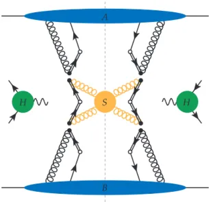
However, actually proving that the dDY cross section can be written in a factorised form requires some work in the soft gluon sector as it has to be shown that just like in the SPS case the soft gluons can be decoupled using appropriate Ward identities which was shown only very recently in reference [36]. In addition to this it also has to be established that contributions from soft gluons in the Glauber momentum region cancel in the complete cross section for which the arguments from SPS using light-cone perturbation theory (LCPT) have to be extended to the situation of double parton scattering in reference [34]. The result of these steps is that the dDY cross section can again be factorised as depicted in figure 2.5. Even in the case of colour singlet production considered here the colour structure of DPS is quite a bit more complicated than in the SPS case. The reason for this is that for a single parton distribution the parton on the left-hand side and the one on the right-hand side have to be coupled to a colour singlet state, whereas in double parton distributions corresponding partons on the left-hand side and right-hand side are not necessarily coupled to a colour singlet.

While it remains true that overall the left-hand side and the right-hand side of the

final state cut have to combine to a colour singlet state this is no longer true for the

2.2. General double parton scattering theory

B A

S H2

H1 H1

H2

Figure2.5.:Factorised cross section for the double Drell-Yan process. The structure is again very similar to the SPS case with the main difference being the two hard subgraphs on each side and the fact that instead of collinear subgraphs with one parton leg on each side of the final state cut identified with a PDF one now has collinear subgraphs with two parton legs on each side of the case corresponding to DPDs.

individual partons which can now be in higher colour representations, leading to colour interference distributions as will be discussed in some more detail below.

Even though so far the more general case of transverse momentum dependent fac- torisation has been considered most of the remainder of this work will be concerned with collinear factorisation and collinear double parton distributions. However, for large values of the interparton distance

parton distributions can be matched onto these collinear distributions as discussed in reference [72]. Since the main topic of this thesis are the double parton distributions – in particular collinear (colour singlet) distributions – it is instructive to give the form of the factorisation formula for this case. At leading order, and for colour singlet DPDs, the factorised collinear cross section is given by

ds

dx

dx

d ¯ x

d ¯ x

= ¹

C Â

a1a2b1b2

s

ˆ

( x

x ¯

s,

)

ˆ

( x

x ¯

s,

)

⇥

Z

d

F

( x ¯

, ¯ x

,

,

)

F

( x

, x

,

,

) , (2.15)

with collinear colour singlet DPDs

F

( x

, x

,

,

) and parton level cross sections

ˆ

( x xs, ¯

) where

is the relative transverse distance between partons a

and a

. In

the above equation C is a combinatorial factor which is equal to 1 of the two observed

final states A and B are different, and equal to 2 if they are indistinguishable. At